
Skin-Friction-Based Identification of the Critical Lines in a Transonic, High Reynolds Number Flow via Temperature-Sensitive Paint


Abstract
:1. Introduction
2. Applied Methods
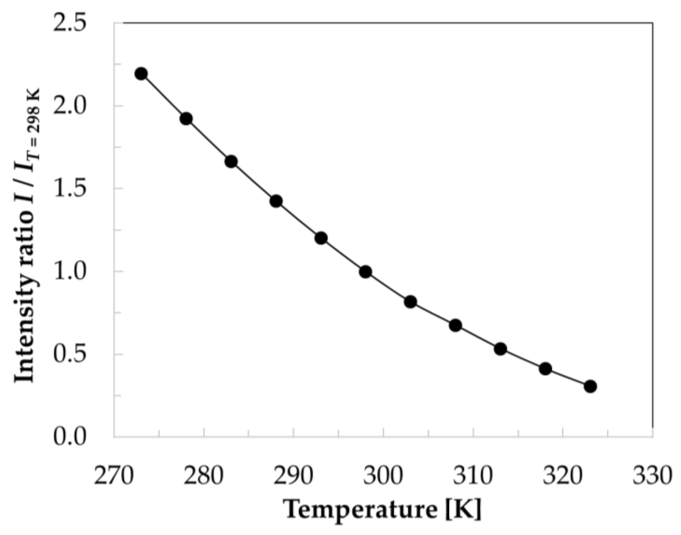
2.1. Temperature-Sensitive Paint Measurement Technique
2.2. Skin-Friction Extraction Methodologies
2.2.1. Approach Based on the Energy Equation at the Wall (OF Approach)
2.2.2. Approaches Based on the Celerity of Propagation of Temperature Perturbations
- Minimization of the dissimilarity from the Taylor Hypothesis (TH approach).
- Tracking of thermal perturbations (TR approach).
- o Densification to compute a dense flow field;
- o Variational refinement of the dense flow field.
3. Experimental Setup
3.1. Transonic Wind Tunnel Göttingen
3.2. Wind-Tunnel Model and Measurement Techniques
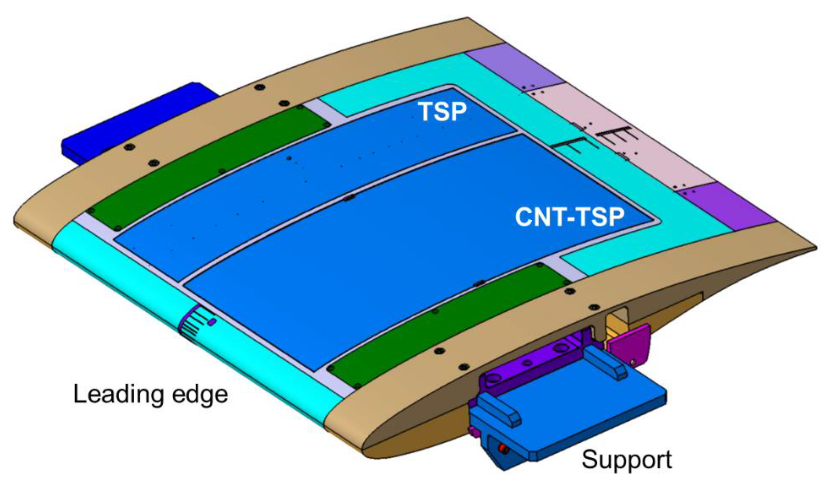
3.2.1. Model Insert with a CNT-Heating (CNT-Insert)
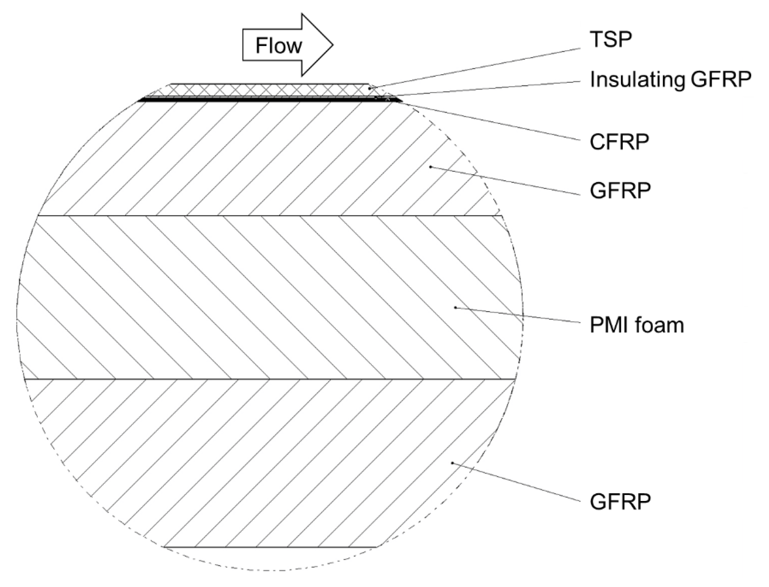
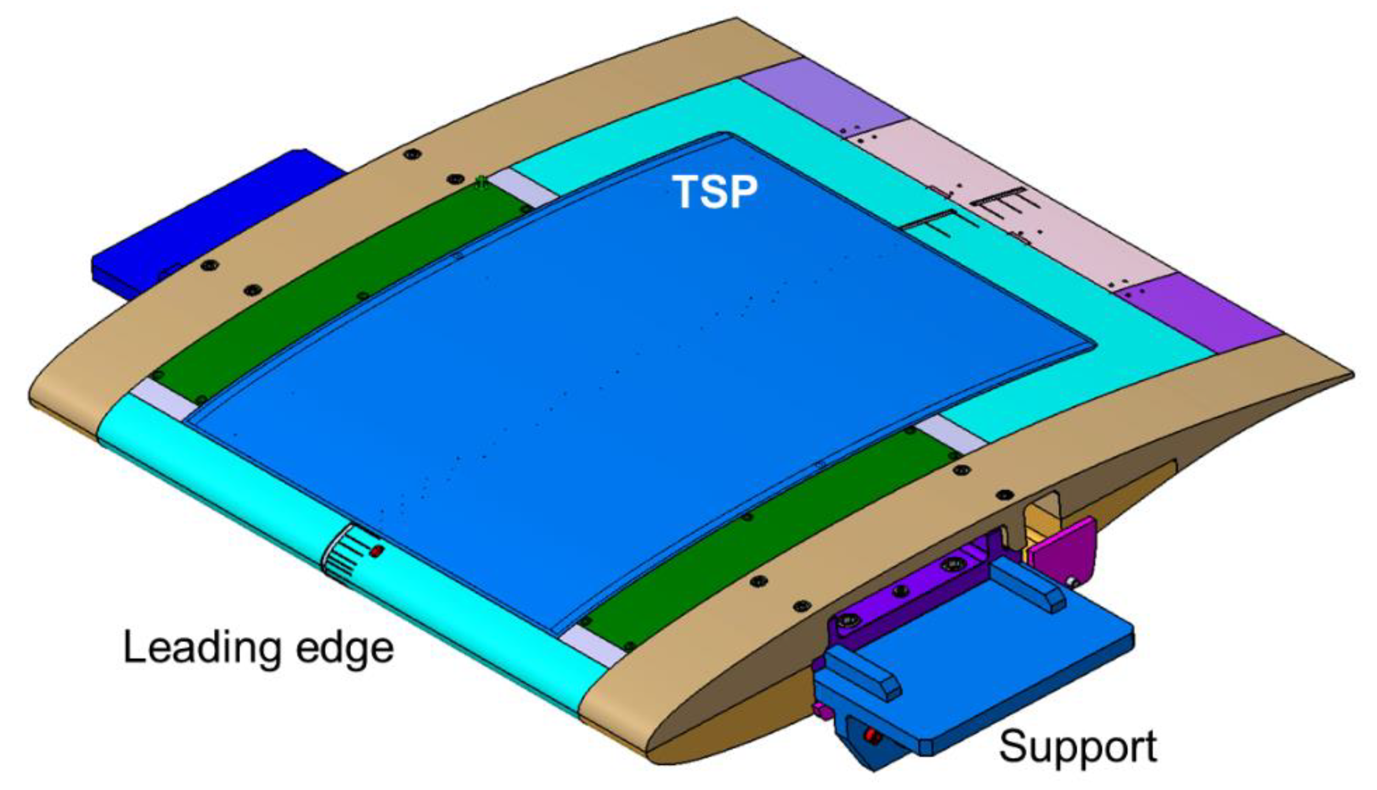
3.2.2. Model Insert with CFRP Heating (CFRP-Insert)
3.3. Optical Setup
- In the first phase of the test campaign, one high-speed camera was used to investigate the model with the CNT-insert. This camera was a Complementary Metal-Oxide-Semiconductor (CMOS) Photron FASTCAM Mini AX200 camera, which has a 12-bit dynamic range and was operated with a 1024 × 672 pixels image sensor. The CMOS camera was equipped with a 24 mm focal length lens and mounted behind one of the circular windows at the starboard test-section wall (see Figure 1). A band-pass filter for the wavelength range of 590–670 nm was mounted in front of the camera lens, thus allowing the light emitted by the TSP to be captured while at the same time blocking light at shorter and higher wavelengths. During this first phase of the experimental campaign, TSP images were acquired at facq = 1 kHz (the camera shutter speed was 1/frame s).
- In the second phase of the test campaign, two Charge-Coupled Device (CCD) pco.4000 cameras were used to investigate the model with the CFRP-insert. They have a 14-bit dynamic range and high spatial resolution (4008 × 2672 pixels image sensor), but also have a relatively low frame rate: in this phase of the experimental campaign, the TSP images were acquired at facq = 3.3 Hz (CCD exposure time of 90 ms). Each camera was equipped with a 24 mm focal length lens, and band-pass spectral filters for the wavelength range of 600–700 nm were mounted between the camera lenses and the CCD chips. One camera was mounted at each test-section side, as shown in Figure 6.
4. TSP Data Acquisition and Processing
4.1. TSP Data Acquisition
4.2. Preprocessing of the TSP Images
4.3. Spatial Filtering of the TSP Data
5. Results and Discussion
5.1. Topology of the Skin-Friction Lines Obtained via the OF Approach
- Tw(x,y) = TRun,avg(x,y);
- Tref(x,y) = Taw(x,y) = TRef,avg(x,y),
5.2. Distributions of Obtained via the TH and TR Approaches
5.2.1. Distributions of Obtained via the TH Approach
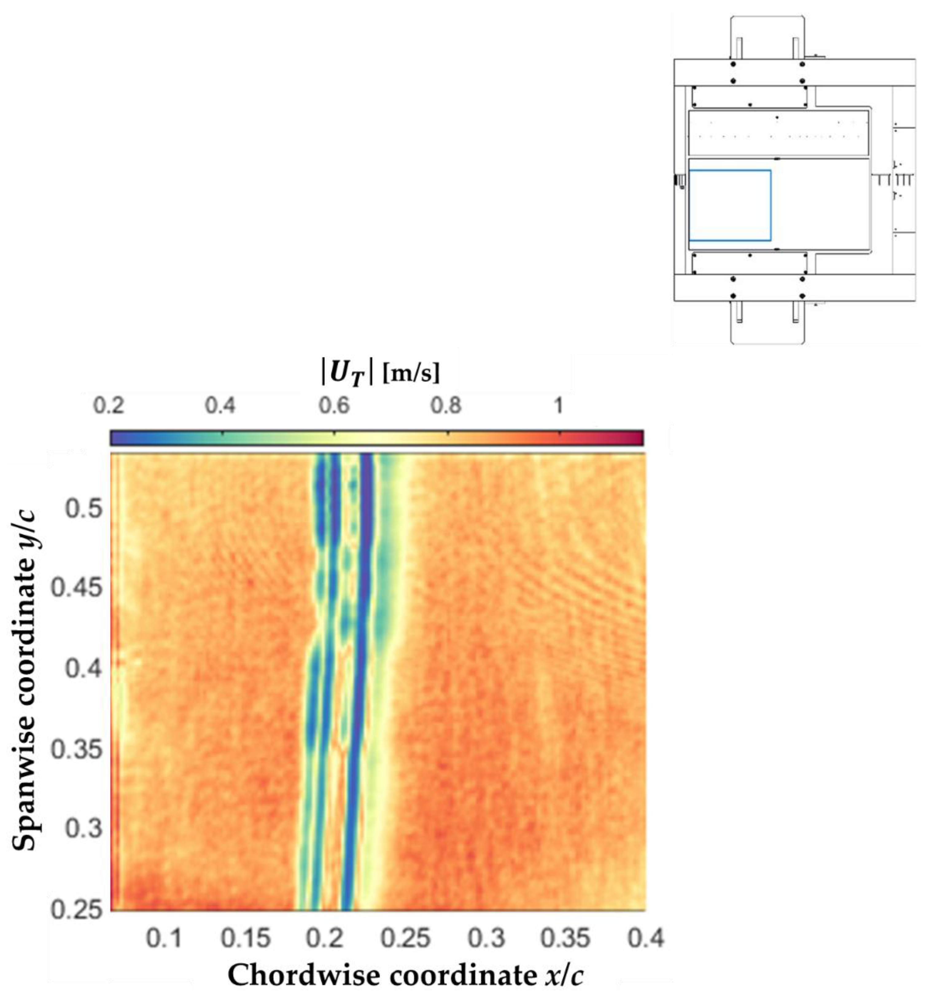
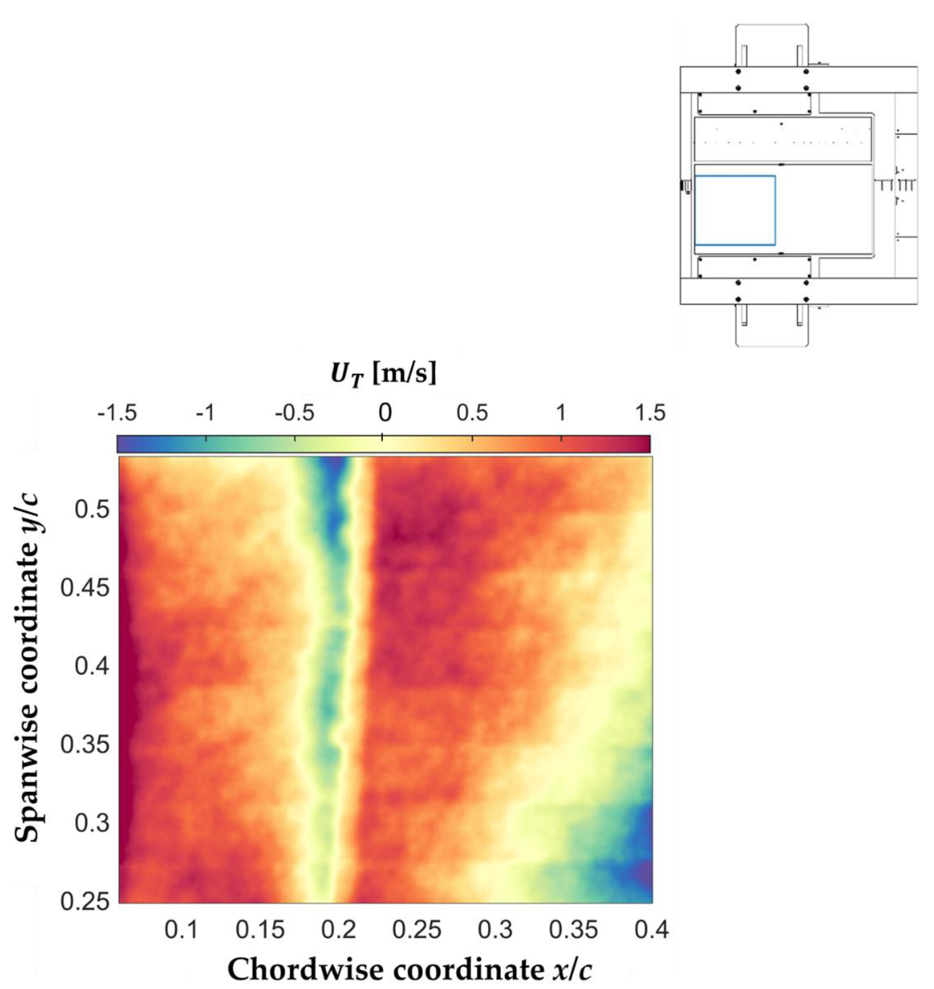
5.2.2. Distributions of Obtained via the TR Approach
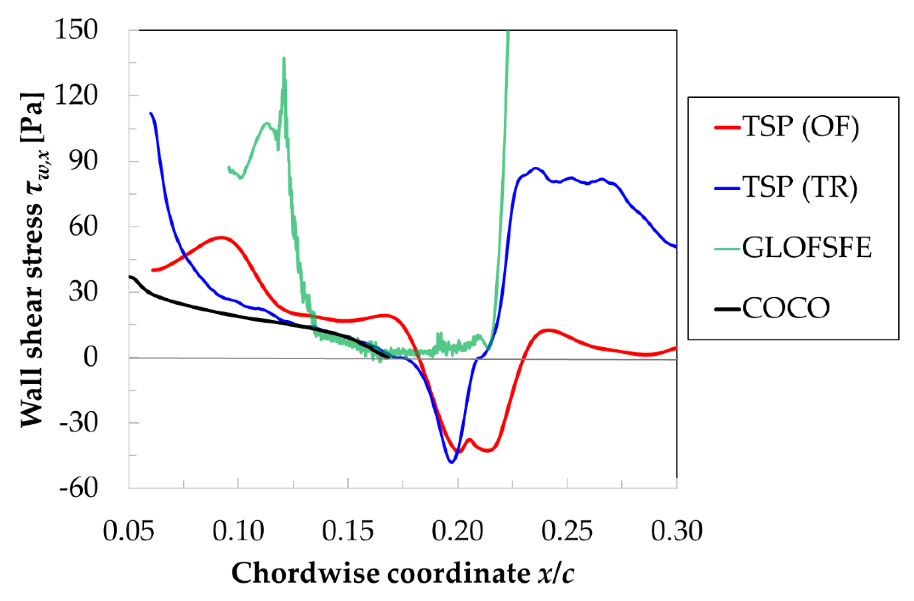
5.3. Comparison of the Detected Critical Locations with Reference Data
5.4. Exploration of the Feasibility to Determine the Quantitative Skin-Friction Distribution via the OF and TR Approaches
6. Conclusions and Recommendations for Future Work
- The imposed heat flux should be as homogeneous and stable as possible. As could be seen in this work, a current-carrying carbon fiber layer appears to be the most promising heating system to impose a uniform heat flux. As compared to the present results, a further improvement in the heat flux uniformity and stability can be achieved by applying a screening layer between the TSP and the current-carrying carbon fiber layers. This adaptation of the layer composition should lead to a compensation of possible heating inhomogeneities.
- The above improvement is expected to lead also to an increase of the signal-to-noise ratio in the turbulent flow region. Nevertheless, for the investigated test conditions with relatively small flow-induced temperature gradients, the surface temperature differences should be further enhanced, for example, by applying the highest electrical power allowed for the safe operation of the current-carrying carbon fiber layer.
- For the study of the potential and of the limits of the approaches relying on time-resolved TSP data (in particular, of the TH approach), it is recommended to perform measurements using a TSP with a shorter response time (e.g., based on a ruthenium complex [103,104]) and to record the TSP data at a higher acquisition frequency (facq of the order of 10 kHz).
- Reference data should also be generated for the turbulent flow region. As discussed in Section 1, the examined flow conditions are challenging for skin-friction measurements, but oil-film interferometry appears to be the most appropriate technique to obtain quantitative skin-friction data in the DNW-TWG, even in the turbulent flow region. It is also suggested to perform numerical simulations that can account for boundary-layer transition and SWBLI, in order to carry out comparisons between the numerical and the experimental results. Note, here, that not only the boundary layer developing on the model surface, but probably also the wind-tunnel environment [89] should be considered.
Author Contributions
Funding
Institutional Review Board Statement
Informed Consent Statement
Data Availability Statement
Acknowledgments
Conflicts of Interest
References
- Lynde, M.N.; Campbell, R.L. Computational Design and Analysis of a Transonic Natural Laminar Flow Wing for a Wind Tunnel Model. In Proceedings of the 35th AIAA Applied Aerodynamics Conference, Denver, CO, USA, 5–9 June 2017. Paper No. 2017-3058. [Google Scholar]
- Liu, Y.; Elham, A.; Horst, P.; Hepperle, M. Exploring Vehicle Level Benefits of Revolutionary Technology Progress via Aircraft Design and Optimization. Energies 2018, 11, 166. [Google Scholar] [CrossRef] [Green Version]
- European Commission. European Aeronautics: A Vision for Report of the Group of Personalities. Available online: https://ec.europa.eu/transport/sites/transport/files/modes/air/doc/flightpath2050.pdf (accessed on 12 March 2021).
- Bezos-O’Connor, G.M.; Mangelsdorf, M.F.; Maliska, H.A.; Washburn, A.E.; Wahls, R.A. Fuel Efficiencies through Airframe Improvements. In Proceedings of the 3rd AIAA Atmospheric Space Environments Conference, Honolulu, HI, USA, 27–30 June 2011. Paper No. 2011-3530. [Google Scholar]
- Costantini, M. Experimental Analysis of Geometric, Pressure Gradient and Surface Temperature Effects on Boundary-Layer Transition in Compressible High Reynolds Number Flow. Ph.D. Thesis, RWTH Aachen, Aachen, Germany, 2016. Available online: https://elib.dlr.de/117965/ (accessed on 12 March 2021).
- Joslin, R.D. Aircraft Laminar Flow Control. Annu. Rev. Fluid Mech. 1998, 30, 1–29. [Google Scholar] [CrossRef] [Green Version]
- Giepman, R.H.M.; Schrijer, F.F.J.; van Oudheusden, B.W. High-resolution PIV measurements of a transitional shock wave–boundary layer interaction. Exp. Fluids 2015, 56, 113. [Google Scholar] [CrossRef] [Green Version]
- Lusher, D.J.; Sandham, N.D. The effect of flow confinement on laminar shock-wave/boundary-layer interactions. J. Fluid Mech. 2020, 897, A18. [Google Scholar] [CrossRef]
- Erdem, E.; Kontis, K.; Johnstone, E.; Murray, N.P.; Steelant, J. Experiments on transitional shock wave–boundary layer interactions at Mach. Exp. Fluids 2013, 54, 1598. [Google Scholar]
- Sivasubramanian, J.; Fasel, H.F. Numerical investigation of shock-induced laminar separation bubble in a Mach 2 boundary layer. In Proceedings of the 45th AIAA Fluid Dynamics Conference, Dallas, TX, USA, 22–26 June 2015. Paper No. 2015-2641. [Google Scholar]
- Babinsky, H.; Harvey, J.K. Shock Wave-Boundary-Layer Interactions; Cambridge University Press: Cambridge, UK, 2011. [Google Scholar]
- Delery, J.M. Shock wave/turbulent boundary layer interaction and its control. Prog. Aerosp. Sci. 1985, 22, 209–280. [Google Scholar] [CrossRef]
- Dolling, D.S. Fifty years of shock-wave/boundary-layer interaction research: What next? AIAA J. 2001, 39, 1517–1531. [Google Scholar] [CrossRef]
- Coschignano, A.; Atkins, N.; Serna, J. Effect of Reynolds number on a normal shock wave-transitional boundary-layer interaction over a curved surface. Exp. Fluids 2019, 60, 185. [Google Scholar] [CrossRef] [Green Version]
- Costantini, M.; Klein, C. Investigation of Shock-Induced Boundary-Layer Transition in Transonic High Reynolds Number Flows Using Temperature-Sensitive Paints. In Proceedings of the 15th International Conference on Fluid Control, Measurements and Visualization (FLUCOME 2019), Naples, Italy, 27–29 May 2019. Paper No. 214. [Google Scholar]
- Sandham, N.; Schülein, E.; Wagner, A.; Willems, S.; Steelant, J. Transitional shock-wave/boundary-layer interactions in hypersonic flow. J. Fluid Mech. 2014, 752, 349–382. [Google Scholar] [CrossRef] [Green Version]
- Davidson, T.S.; Babinsky, H. Influence of Boundary-Layer State on Development Downstream of Normal Shock Interactions. AIAA J. 2018, 56, 2298–2307. [Google Scholar] [CrossRef] [Green Version]
- Mayle, R.E. The role of laminar–turbulent transition in gas turbine engines. J. Turbomach. 1991, 113, 509–536. [Google Scholar] [CrossRef]
- Coschignano, A.; Babinsky, H.; Sheaf, C.; Zamboni, G. Normal shock-boundary layer interactions in transonic intakes at high incidence. AIAA J. 2019, 57, 2867–2880. [Google Scholar] [CrossRef]
- Görtz, S.; Krumbein, A.; Ritter, M.R.; Hofmann, J. Ergebnisse des DLR-Projekts VicToria—Virtual Aircraft Technology Integration Platform. In Proceedings of the Deutscher Luft- und Raumfahrtkongress 2020 (DLRK2020), Virtual Event, 1–3 September 2020. [Google Scholar]
- Liu, T.; Montefort, J.; Woodiga, S.; Merati, P.; Shen, L. Global luminescent oil-film skin-friction meter. AIAA J. 2008, 46, 476–485. [Google Scholar] [CrossRef]
- Lighthill, M.J. Introduction: Boundary Layer Theory. In Laminar Boundary Layers; Rosenhead, L., Ed.; Oxford University Press: Oxford, UK, 1963; Part 2. [Google Scholar]
- Delery, J.M. Three-dimensional separated flows topology. In Critical Points, Separation Lines and Vortical Structures, Focus Series in Fluid Mechanics; Wiley: Hoboken, NJ, USA, 2013. [Google Scholar]
- Miozzi, M.; Capone, A.; Di Felice, F.; Klein, C.; Liu, T. Global and local skin friction diagnostics from TSP surface patterns on an underwater cylinder in crossflow. Phys. Fluids 2016, 28, 124101. [Google Scholar] [CrossRef]
- Miozzi, M.; Capone, A.; Costantini, M.; Fratto, L.; Klein, C.; Di Felice, F. Skin friction and coherent structures within a laminar separation bubble. Exp. Fluids 2019, 60, 13. [Google Scholar] [CrossRef]
- Liu, T. Global skin friction measurements and interpretation. Prog. Aerosp. Sci. 2019, 111, 100584. [Google Scholar] [CrossRef]
- Löfdahl, L.; Gad-el Hak, M. MEMS-based pressure and shear stress sensors for turbulent flows. Meas. Sci. Technol. 1999, 10, 665–686. [Google Scholar] [CrossRef] [Green Version]
- Naughton, J.W.; Sheplak, M. Modern developments in shear-stress measurement. Prog. Aerosp. Sci. 2002, 38, 515–570. [Google Scholar] [CrossRef]
- Plesniak, M.; Peterson, S. Wall shear stress measurements for conventional applications and biomedical flows. In Proceedings of the 24th AIAA Aerodynamic Measurement Technology and Ground Testing Conference, Portland, OR, USA, 28 June–1 July 2004. Paper No. 2004-2301. [Google Scholar]
- Klewicki, J.C. Measurement of Wall Shear Stress. In Springer Handbook of Experimental Fluid Mechanics; Tropea, C., Yarin, A.L., Foss, J.F., Eds.; Springer: Berlin, Germany, 2007; Chapter 12.2. [Google Scholar]
- Hakkinen, R.J. Reflections on Fifty Years of Skin Friction Measurement. In Proceedings of the 24th AIAA Aerodynamic Measurement Technology and Ground Testing Conference, Portland, OR, USA, 28 June–1 July 2004. Paper No. 2004-2111. [Google Scholar]
- Ding, G.-H.; Ma, B.-H.; Deng, J.-J.; Yuan, W.-Z.; Liu, K. Accurate Measurements of Wall Shear Stress on a Plate with Elliptic Leading Edge. Sensors 2018, 18, 2682. [Google Scholar] [CrossRef] [Green Version]
- Ludwieg, H. Instrument for Measuring the Wall Shearing Stress of Turbulent Boundary Layers; NASA: Washington, DC, USA, 1950. [Google Scholar]
- Meijering, A.; Schröder, W. viExperimental Analysis of Separated Transitional Transonic Airfoil Flow. In Proceedings of the 15th AIAA Computational Fluid Dynamics Conference, Anaheim, CA, USA, 11–14 June 2001. Paper No. 2001-2987. [Google Scholar]
- Burkhardt, O. Erprobung und Anwendung von Oberflächensensoren und Sensorarrays zur Erfassung instationärer Wandschubspannungen an Schaufelprofilen. Ph.D. Thesis, TU Berlin, Berlin, Germany, 2004. [Google Scholar]
- Preston, J.H. The Determination of Turbulent Skin Friction by Means of Pitot Tubes. J. R. Aeronaut. Soc. 1954, 58, 109–121. [Google Scholar] [CrossRef]
- Kähler, C.J.; Scholz, U.; Ortmanns, J. Wall-shear-stress and near-wall turbulence measurements up to single pixel resolution by means of long-distance micro-PIV. Exp. Fluids 2006, 41, 327–341. [Google Scholar] [CrossRef]
- Novara, M.; Schanz, D.; Geisler, R.; Gesemann, S.; Voss, C.; Schröder, A. Multi-Exposed recordings for 3D Lagrangian Particle Tracking with Multi-Pulse Shake-The-Box. Exp. Fluids 2019, 60, 44. [Google Scholar] [CrossRef] [Green Version]
- Clauser, F.H. Turbulent Boundary Layers in Adverse Pressure Gradients. J. Aeronaut. Sci. 1954, 21, 91–108. [Google Scholar] [CrossRef]
- Tanner, L.H.; Blows, L.G. A study of the motion of oil films on surfaces in air flow, with application to the measurement of skin friction. J. Phys. E Sci. Instrum. 1976, 9, 194–202. [Google Scholar] [CrossRef]
- Naughton, J.W.; Brown, J.L. Surface interferometric skin-friction measurement technique. In Proceedings of the Advanced measurement and ground testing conference, New Orleans, LA, USA, 17–20 June 1996. Paper No. 1996-2183. [Google Scholar]
- Lunte, J.; Schülein, E. Wall shear stress measurements by white-light oil-film interferometry. Exp. Fluids 2020, 61, 84. [Google Scholar] [CrossRef] [Green Version]
- Schülein, E. Optical skin friction measurements in the short-duration Ludwieg tube facility. In Proceedings of the 20th International Congress on Instrumentation in Aerospace Simulation Facilities, ICIASF 03, Göttingen, Germany, 25–29 August 2003; pp. 157–168. [Google Scholar]
- Mosharov, V.; Radchenko, V.; Klein, C.; Henne, U.; Kirmse, T. Evaluation of PISFV method in subsonic wind tunnel. In Proceedings of the 11th International Conference on Fluid Control, Measurements and Visualization (FLUCOME 2011), Keelung, Taiwan, 5–9 December 2011. Paper No. 23. [Google Scholar]
- Mosharov, V.; Radchenko, V. PIV on the surface. In Proceedings of the 10th International Symposium on Particle Image Velocimetry—PIV13, Delft, The Netherlands, 1–3 July 2013. Paper No. A037. [Google Scholar]
- Husen, N.M.; Roozeboom, N.; Liu, T.; Sullivan, J.P. Global skin-friction measurements using particle image surface flow visualization and a luminescent oil-film. In Proceedings of the 53rd AIAA Aerospace Sciences Meeting, Kissimmee, FL, USA, 5–9 January 2015. Paper No. 2015-0022. [Google Scholar]
- Lee, T.; Nonomura, T.; Asai, K.; Liu, T. Linear least-squares method for global luminescent oil film skin friction field analysis. Rev. Sci. Instrum. 2018, 89, 065106. [Google Scholar] [CrossRef] [PubMed]
- Costantini, M.; Lee, T.; Nonomura, T.; Asai, K.; Klein, C. Feasibility of skin-friction field measurements in a transonic wind tunnel using a global luminescent oil film. Exp. Fluids 2021, 62, 21. [Google Scholar] [CrossRef]
- Lo, K.H.; Kontis, K. Flow visualisation of a normal shock impinging over a rounded contour bump in a Mach 1.3 free-stream. J. Vis. 2017, 20, 237–249. [Google Scholar] [CrossRef] [PubMed] [Green Version]
- Drake, A.; Kennelly, R.A., Jr. In-Flight Skin Friction Measurements Using Oil Film Interferometry. J. Aircraft 1999, 36, 723–725. [Google Scholar] [CrossRef]
- Grosse, S.; Schröder, W. The Micro-Pillar Shear-Stress Sensor MPS3 for Turbulent Flow. Sensors 2009, 9, 2222–2251. [Google Scholar] [CrossRef]
- Liu, Y.; Klaas, M.; Schröder, W. Measurements of the wall-shear stress distribution in turbulent channel flow using the micro-pillar shear stress sensor MPS3. Exp. Therm. Fluid Sci. 2019, 106, 171–182. [Google Scholar] [CrossRef]
- Fonov, S.D.; Jones, G.; Crafton, J.; Fonov, V.; Goss, L. The Development of Optical Technique for the Measurement of Pressure and Skin Friction. Meas. Sci. Technol. 2006, 17, 1261–1268. [Google Scholar] [CrossRef]
- Reda, D.C.; Wilder, M.C.; Farina, D.J.; Zilliac, G. New Methodology for the Measurement of Surface Shear Stress Vector Distributions. AIAA J. 1997, 35, 608–614. [Google Scholar] [CrossRef]
- Zhao, J. Measurement of Wall Shear Stress in High Speed Air Flow Using Shear-Sensitive Liquid Crystal Coating. Sensors 2018, 18, 1605. [Google Scholar] [CrossRef] [Green Version]
- Liu, T.; Woodiga, S.A. Feasibility of global skin friction diagnostics using temperature sensitive paint. Meas. Sci. Technol. 2011, 22, 115402. [Google Scholar] [CrossRef]
- Miozzi, M.; Di Felice, F.; Klein, C.; Costantini, M. Taylor hypothesis applied to direct measurement of skin friction using data from Temperature Sensitive Paint. Exp. Therm. Fluid Sci. 2020, 110, 109913. [Google Scholar] [CrossRef]
- Miozzi, M.; Costantini, M. Temperature and skin-friction maps on a lifting hydrofoil in a propeller wake. Meas. Sci. Techol. 2021, in press. [Google Scholar] [CrossRef]
- Liu, T. Extraction of skin-friction fields from surface flow visualizations as an inverse problem. Meas. Sci. Technol. 2013, 24, 124004. [Google Scholar] [CrossRef]
- Capone, A.; Klein, C.; Di Felice, F.; Beifuss, U.; Miozzi, M. Fast-response underwater TSP investigation of subcritical instabilities of a cylinder in crossflow. Exp. Fluids 2015, 56, 196. [Google Scholar] [CrossRef]
- Krenkel, L. Untersuchung des Einflusses von Wirbelgeneratoren auf die Stoß-/Grenzschicht-Wechselwirkung. Ph.D. Thesis, RWTH Aachen, Aachen, Germany, 2012. [Google Scholar]
- Leuckert, J. Vergleichende Untersuchungen über die Eignung flächiger Sensorarrays zur Charakterisierung instationärer Strömungsphänomene in kompressiblen Strömungen. Ph.D. Thesis, TU Berlin, Berlin, Germany, 2012. [Google Scholar]
- Liu, T.; Sullivan, J.P. Pressure and Temperature Sensitive Paint. Springer: Berlin, Germany, 2005; Chapters 1–4 and 8. [Google Scholar]
- Fey, U. Transition-Detection by Temperature-Sensitive Paint. In Springer Handbook of Experimental Fluid Mechanics; Tropea, C., Yarin, A.L., Foss, J.F., Eds.; Springer: Berlin, Germany, 2007; Chapter 7.4. [Google Scholar]
- Costantini, M.; Fuchs, C.; Henne, U.; Klein, C.; Ondrus, V.; Bruse, M.; Löhr, M.; Jacobs, M. Experimental Analysis of the Performance of a Wind-Turbine Airfoil Using Temperature-Sensitive Paint. AIAA J. 2021, in press. [Google Scholar] [CrossRef]
- Asai, K.; Kanda, H.; Kunimasu, T.; Liu, T.; Sullivan, J.P. Boundary-Layer Transition Detection in a Cryogenic Wind Tunnel Using Luminescent Paint. J. Aircr. 1997, 34, 34–42. [Google Scholar] [CrossRef]
- Egami, Y.; Fey, U.; Klein, C.; Sitzmann, M.; Wild, J. Transition Detection on High-Lift Devices in DNW-KKK by Means of Temperature-Sensitive Paint. In Proceedings of the 12th International Symposium on Flow Visualization, DLR. Göttingen, Germany, 10–14 September 2006. Paper 237. [Google Scholar]
- Egami, Y.; Klein, C.; Henne, U.; Bruse, M.; Ondrus, V.; Beifuss, U. Development of a Highly Sensitive Temperature-Sensitive Paint for Measurements under Ambient (0–60 °C) Conditions. In Proceedings of the 47th AIAA Aerospace Sciences Meeting including The New Horizons Forum and Aerospace Exposition, Orlando, FL, USA, 5–8 January 2009. Paper No. 2009-1075. [Google Scholar]
- Costantini, M.; Fey, U.; Henne, U.; Klein, C. Nonadiabatic Surface Effects on Transition Measurements Using Temperature-Sensitive Paints. AIAA J. 2015, 53, 1172–1187. [Google Scholar] [CrossRef]
- Klein, C.; Henne, U.; Sachs, W.E.; Beifuss, U.; Ondrus, V.; Bruse, M.; Lesjak, R.; Löhr, M.; Becher, A.; Zhai, J. Combination of Temperature-Sensitive Paint (TSP) and Carbon Nanotubes (CNT) for Transition Detection. In Proceedings of the 53rd AIAA Aerospace Sciences Meeting, Kissimmee, FL, USA, 5–9 January 2015. Paper No. 2015-1558. [Google Scholar]
- Goodman, K.Z.; Lipford, W.E.; Watkins, A.N. Boundary-Layer Detection at Cryogenic Conditions Using Temperature Sensitive Paint Coupled with a Carbon Nanotube Heating Layer. Sensors 2016, 16, 2062. [Google Scholar] [CrossRef] [PubMed] [Green Version]
- Klein, C.; Henne, U.; Yorita, D.; Beifuss, U.; Ondrus, V.; Hensch, A.-K.; Longo, R.; Hauser, M.; Guntermann, P.; Quest, J. Application of Carbon Nanotubes and Temperature-Sensitive Paint for the Detection of Boundary Layer Transition under Cryogenic Conditions. In Proceedings of the 55th AIAA Aerospace Sciences Meeting, Grapevine, TX, USA, 9–13 January 2017. Paper No. 2017-0336. [Google Scholar]
- Lemarechal, J.; Klein, C.; Henne, U.; Puckert, D.K.; Rist, U. Detection of Lambda- and Omega-vortices with the temperature-sensitive paint method in the late stage of controlled laminar–turbulent transition. Exp. Fluids 2019, 60, 19. [Google Scholar] [CrossRef]
- Petzold, R.; Radespiel, R. Transition on a wing with spanwise varying crossflow and linear stability analysis. AIAA J. 2015, 53, 321–335. [Google Scholar] [CrossRef]
- Miozzi, M.; Capone, A.; Klein, C.; Costantini, M. Incipient stall characterization from skin friction maps. Int. J. Numer. Methods Heat Fluid Flow 2020. [Google Scholar] [CrossRef]
- Horn, B.K.P.; Schunck, B.G. Determining optical flow. Artif. Intell. 1981, 17, 185–204. [Google Scholar] [CrossRef] [Green Version]
- Schlichting, H.; Gersten, K. Boundary-Layer Theory, 8th ed.; Springer: Berlin, Germany, 2016; Chapters 9, 10, 18 and 19. [Google Scholar]
- Eckelmann, H. The structure of the viscous sublayer and the adjacent wall region in a turbulent channel flow. J. Fluid Mech. 1974, 65, 439–459. [Google Scholar] [CrossRef]
- Kim, J.; Hussain, F. Propagation velocity of perturbations in turbulent channel flow. Phys. Fluids A 1993, 5, 695–706. [Google Scholar] [CrossRef]
- Hetsroni, G.; Tiselj, I.; Bergant, R.; Mosyak, A.; Pogrebnyak, E. Convection velocity of temperature fluctuations in a turbulent flume. J. Heat Transf. 2004, 126, 843–848. [Google Scholar] [CrossRef]
- Taylor, G.I. The spectrum of turbulence. Proc. R. Soc. Lond. A Math. Phys. Sci. 1938, 164, 476–490. [Google Scholar] [CrossRef] [Green Version]
- Del Alamo, J.C.; Jimenez, J. Estimation of turbulent convection velocities and corrections to Taylor’s approximation. J. Fluid Mech. 2009, 640, 5–26. [Google Scholar] [CrossRef]
- Geng, C.; He, G.; Wang, Y.; Xu, C.; Lozano-Duran, A.; Wallace, J.M. Taylor’s hypothesis in turbulent channel flow considered using a transport equation analysis. Phys. Fluids 2015, 27, 025111. [Google Scholar] [CrossRef] [Green Version]
- Kroeger, T.; Timofte, R.; Dai, D.; Van Gool, L. Fast Optical Flow Using Dense Inverse Search. Computer Vision—ECCV 2016; Leibe, B., Matas, J., Sebe, N., Welling, M., Eds.; Springer International Publishing: Cham, Switzerland, 2016; pp. 471–488. [Google Scholar]
- Baker, S.; Matthews, I. Lucas-Kanade 20 years on: A unifying framework. Int. J. Comput. Vis. 2004, 56, 221–255. [Google Scholar] [CrossRef]
- Lucas, B.D.; Kanade, T. An iterative image registration technique with an application to stereo vision. In Proceedings Darpa Image Understanding Workshop—Volume 2; Morgan Kaufmann Publishers Inc.: San Francisco, CA, USA, 1981; pp. 674–679. [Google Scholar]
- Binder, B.; Riethmueller, L.; Tusche, S.; Wulf, R. Die Modernisierung des Transsonischen Windkanals in Göttingen. In Proceedings of the DGLR-Jahrestagung, Bremen, Germany, 29 September–2 October 1992. Paper No. DGLR-92-03-071. [Google Scholar]
- Amecke, J. Direct Calculation of Wall Interferences and Wall Adaptation for Two-Dimensional Flow in Wind Tunnels with Closed Walls; Tech. Mem. 88523; NASA: Washington, DC, USA, 1986. [Google Scholar]
- Weiand, P.; Michelis, S.; Gardner, A.D. Numerical simulation of an adaptive wall in a virtual transonic wind tunnel. AIAA J. 2017, 55, 3214–3218. [Google Scholar] [CrossRef]
- Barlow, J.B.; Rae, W.H., Jr.; Pope, A. Pressure, Flow, and Shear Stress Measurements. In Low-Speed Wind Tunnel Testing, 3rd ed.; Wiley: New York, NY, USA, 1999; Chapter 4. [Google Scholar]
- Thiede, P.; Krogmann, P.; Stanewsky, E. Active and Passive Shock/Boundary Layer Interaction Control on Supercritical Airfoils; AGARD CP-365; Deutsche Forschungs-und Versuchsanstalt Fuer luft-und Raumfahrt ev Goettingen (Germany fr): Göttingen, Germany, 1984; pp. 24-1–24-13. [Google Scholar]
- Krogmann, P.; Stanewsky, E.; Thiede, P. Transonic shock/boundary layer interaction control. In Proceedings of the 14th Congress of ICAS, Toulouse, France, 9–14 September 1984. Paper No. 84-2.3.2. [Google Scholar]
- Mateer, G.G.; Seegmiller, H.L.; Hand, L.A.; Szodruch, J.A. Experimental Investigation of a Supercritical Airfoil at Transonic Speeds; Tech. Mem. 103933; NASA: Moffett Field, CA, USA, 1992. [Google Scholar]
- Fink, H. Konzipierung eines TSP-Einsatzes mit Integrierter CFK-Heizung für das 1000mm-Profil. Master’s Thesis, University of Applied Sciences and Arts (HAWK), Göttingen, Germany, 2019. [Google Scholar]
- Ondrus, V.; Meier, R.; Klein, C.; Henne, U.; Schäferling, M.; Beifuss, U. Europium 1,3-di(thienyl)propane-1,3-diones with Outstanding Properties for Temperature Sensing. Sens. Actuators A Phys. 2015, 233, 434–441. [Google Scholar] [CrossRef]
- Fink, H. Thermal Analysis of a Wind Tunnel Model with an Integrated CFRP-Heating-Layer; DLR Rep. IB-AS-GO-2021-27; DLR: Göttingen, Germany, 2021. [Google Scholar]
- Klein, C.; Engler, R.H.; Henne, U.; Sachs, W.E. Application of pressure-sensitive paint for determination of the pressure field and calculation of the forces and moments of models in a wind tunnel. Exp. Fluids 2005, 39, 475–483. [Google Scholar] [CrossRef]
- Costantini, M.; Miozzi, M.; Henne, U.; Klein, C. Transition study on supercritical airfoil in compressible high-Reynolds number flow via Temperature-Sensitive Paint. In Proceedings of the 25th International Congress of Theoretical and Applied Mechanics (ICTAM2020+1), IUTAM. Milan, Italy, 23–28 August 2020. [Google Scholar]
- Costantini, M.; Henne, U.; Risius, S.; Klein, C. A Robust Method for Reliable Transition Detection in Temperature-Sensitive Paint Data. Aerosp. Sci. Technol. 2021, 113, 106702. [Google Scholar] [CrossRef]
- Shinde, V.; McNamara, J.; Gaitonde, D.; Barnes, C.; Visbal, M. Transitional shock wave boundary layer interaction over a flexible panel. J. Fluids Struct. 2019, 90, 263–285. [Google Scholar] [CrossRef]
- Sansica, A.; Sandham, N.D.; Hu, Z. Forced response of a laminar shock-induced separation bubble. Phys. Fluids 2014, 26, 093601. [Google Scholar] [CrossRef]
- Schrauf, G. COCO—A Program to Compute Velocity and Temperature Profiles for Local and Nonlocal Stability Analysis of Compressible, Conical Boundary Layers with Suction; ZARM Technik Report; ZARM: Bremen, Germany, 1998. [Google Scholar]
- Ohmi, S.; Nagai, H.; Asai, K.; Nakakita, K. Effect of TSP Layer Thickness on Global Heat Transfer Measurement in Hypersonic Flow. In Proceedings of the 44th AIAA Aerospace Sciences Meeting and Exhibit, Reno, NV, USA, 9–12 January 2006. Paper No. 2006-1048. [Google Scholar]
- Ozawa, H.; Laurence, S.J.; Martinez Schramm, J.; Wagner, A.; Hannemann, K. Fast-response temperature-sensitive-paint measurements on a hypersonic transition cone. Exp. Fluids 2015, 56, 1853. [Google Scholar] [CrossRef]


| Data | xS/c [%] | Δ(xS/c) [%] | xR/c [%] | Δ(xR/c) [%] |
|---|---|---|---|---|
| OF approach (CNT-insert) | 18.2 | ±0.7 | 23.0 | ±1.0 |
| TH approach (CNT-insert) | 19.6 | ±1.0 | 22.5 | ±1.0 |
| TR approach (CNT-insert) | 17.4 | ±0.7 | 21.0 | ±0.5 |
| COCO (CNT-insert) | 16.8 | - | - | - |
| GLOFSFE [48] | 16.5 | ±1.5 | 21.7 | ±1.0 |
| OF approach (CFRP-insert) | 19.6 | ±0.5 | 22.1 | ±0.7 |
| COCO (CFRP-insert) | 19.8 | - | - | - |
Publisher’s Note: MDPI stays neutral with regard to jurisdictional claims in published maps and institutional affiliations. |
© 2021 by the authors. Licensee MDPI, Basel, Switzerland. This article is an open access article distributed under the terms and conditions of the Creative Commons Attribution (CC BY) license (https://creativecommons.org/licenses/by/4.0/).
Share and Cite
Costantini, M.; Henne, U.; Klein, C.; Miozzi, M. Skin-Friction-Based Identification of the Critical Lines in a Transonic, High Reynolds Number Flow via Temperature-Sensitive Paint. Sensors 2021, 21, 5106. https://doi.org/10.3390/s21155106
Costantini M, Henne U, Klein C, Miozzi M. Skin-Friction-Based Identification of the Critical Lines in a Transonic, High Reynolds Number Flow via Temperature-Sensitive Paint. Sensors. 2021; 21(15):5106. https://doi.org/10.3390/s21155106
Chicago/Turabian StyleCostantini, Marco, Ulrich Henne, Christian Klein, and Massimo Miozzi. 2021. "Skin-Friction-Based Identification of the Critical Lines in a Transonic, High Reynolds Number Flow via Temperature-Sensitive Paint" Sensors 21, no. 15: 5106. https://doi.org/10.3390/s21155106