
Spectral Domain Sparse Representation for DOA Estimation of Signals with Large Dynamic Range

Abstract
:1. Introduction
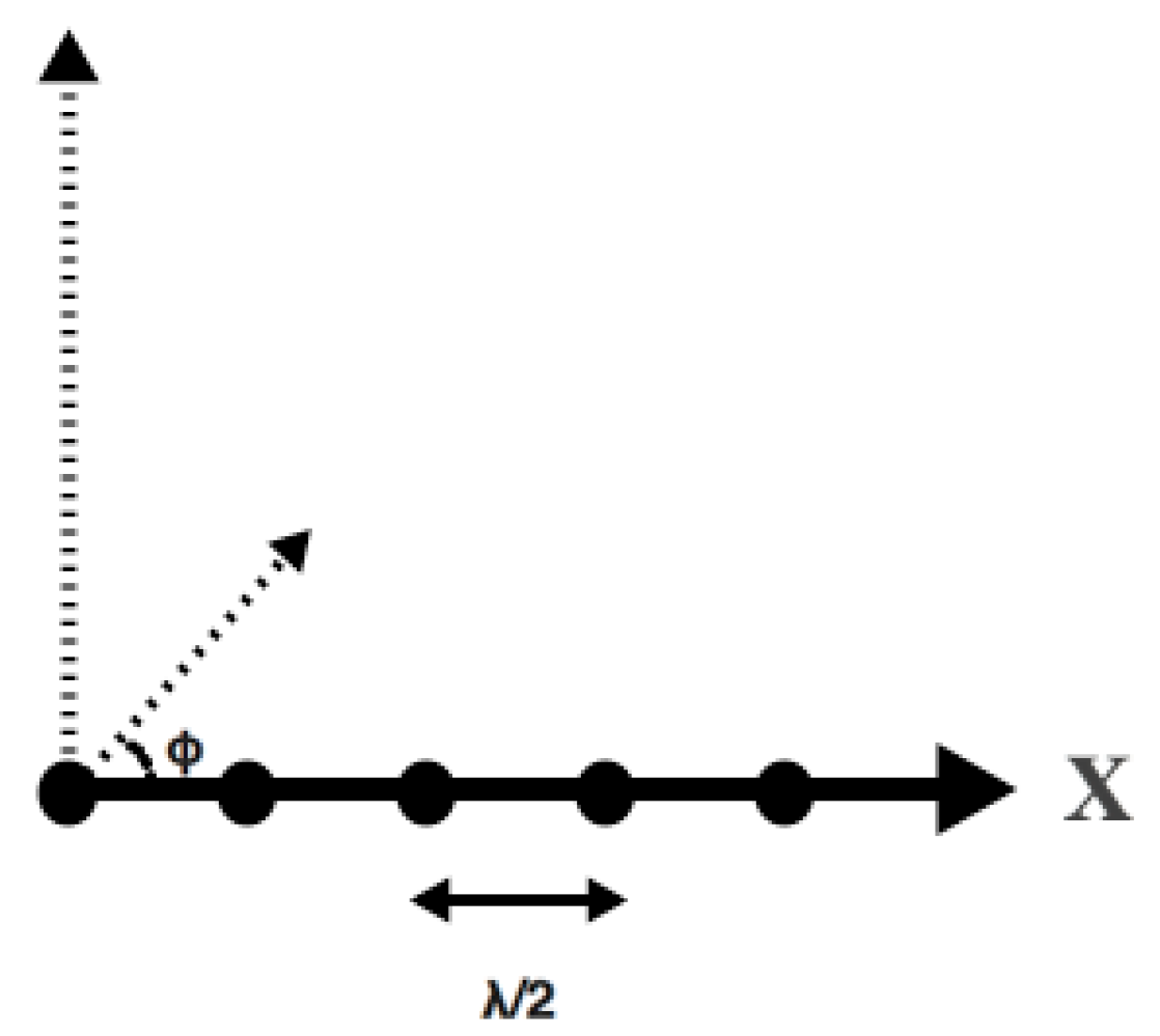
2. Signal Model
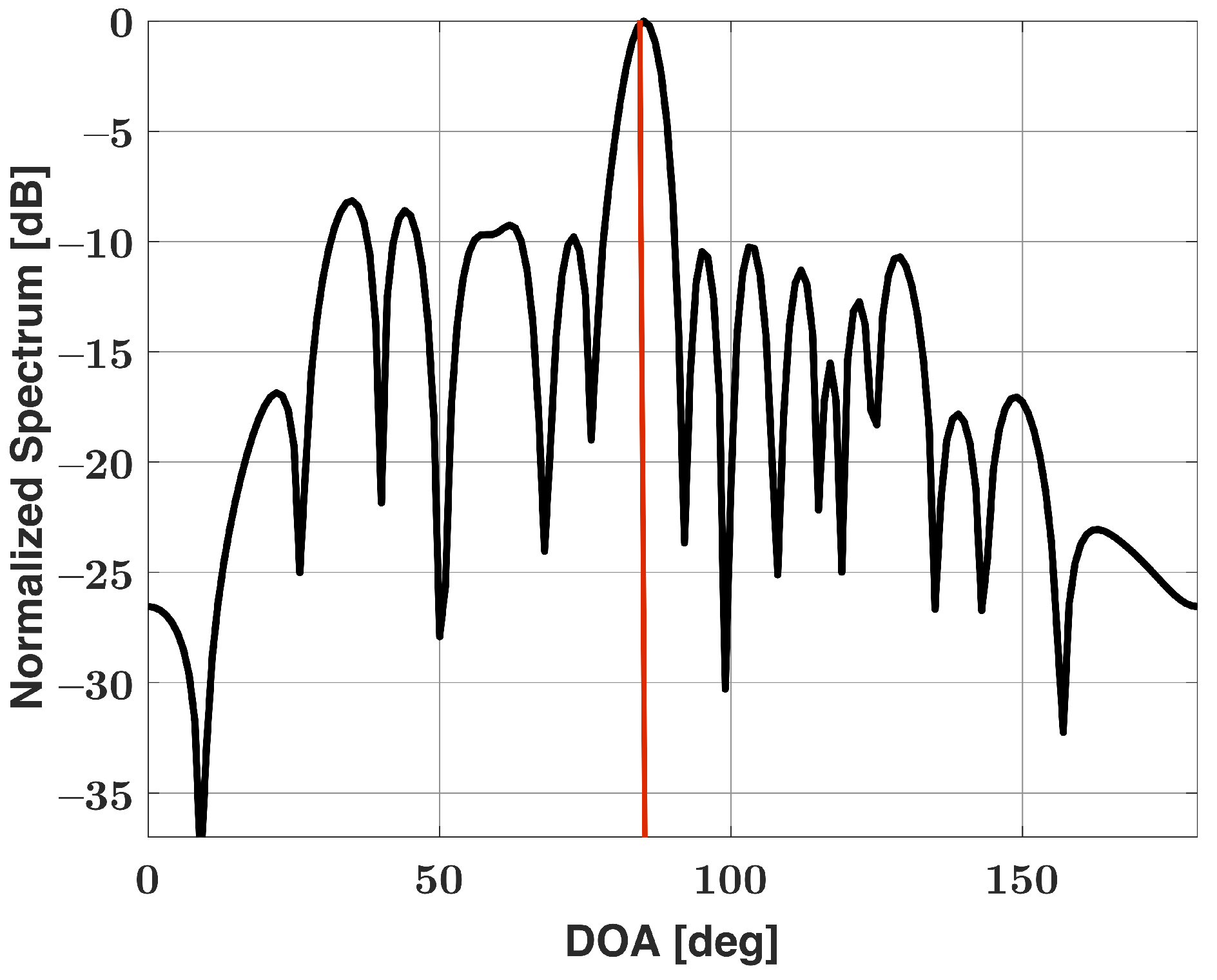
3. Review of SDSR Method
4. Modifications to SDSR Method
4.1. Two-Step Method
4.2. Windowed Bartlett Spectra
4.3. Mixed Windowed Bartlett Spectra
| Algorithm 1 Mixed Windowed Bartlett Spectra SDSR |
| for to do |
| Store which window function is the minimum at each angle . Let this window function be . |
| end for |
| Generate using the window function for each assumed emitter location. |
| such that |
5. Results
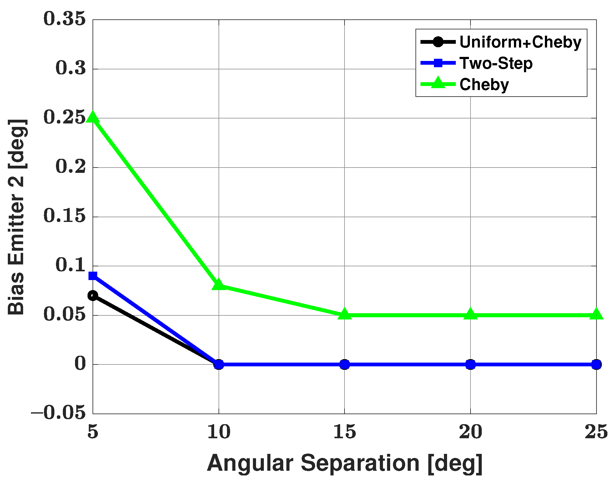
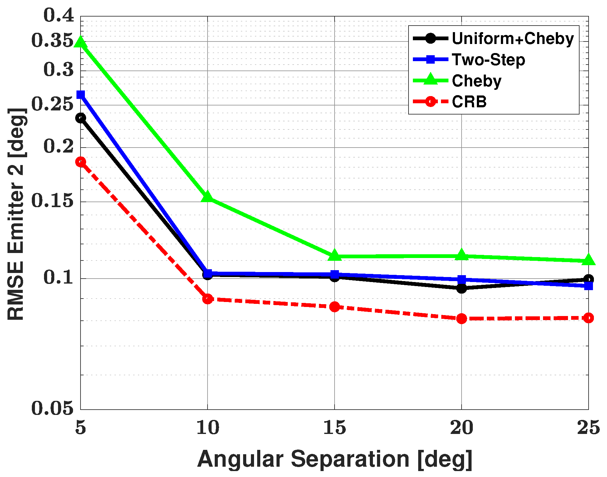
5.1. Two-Signal Scenario
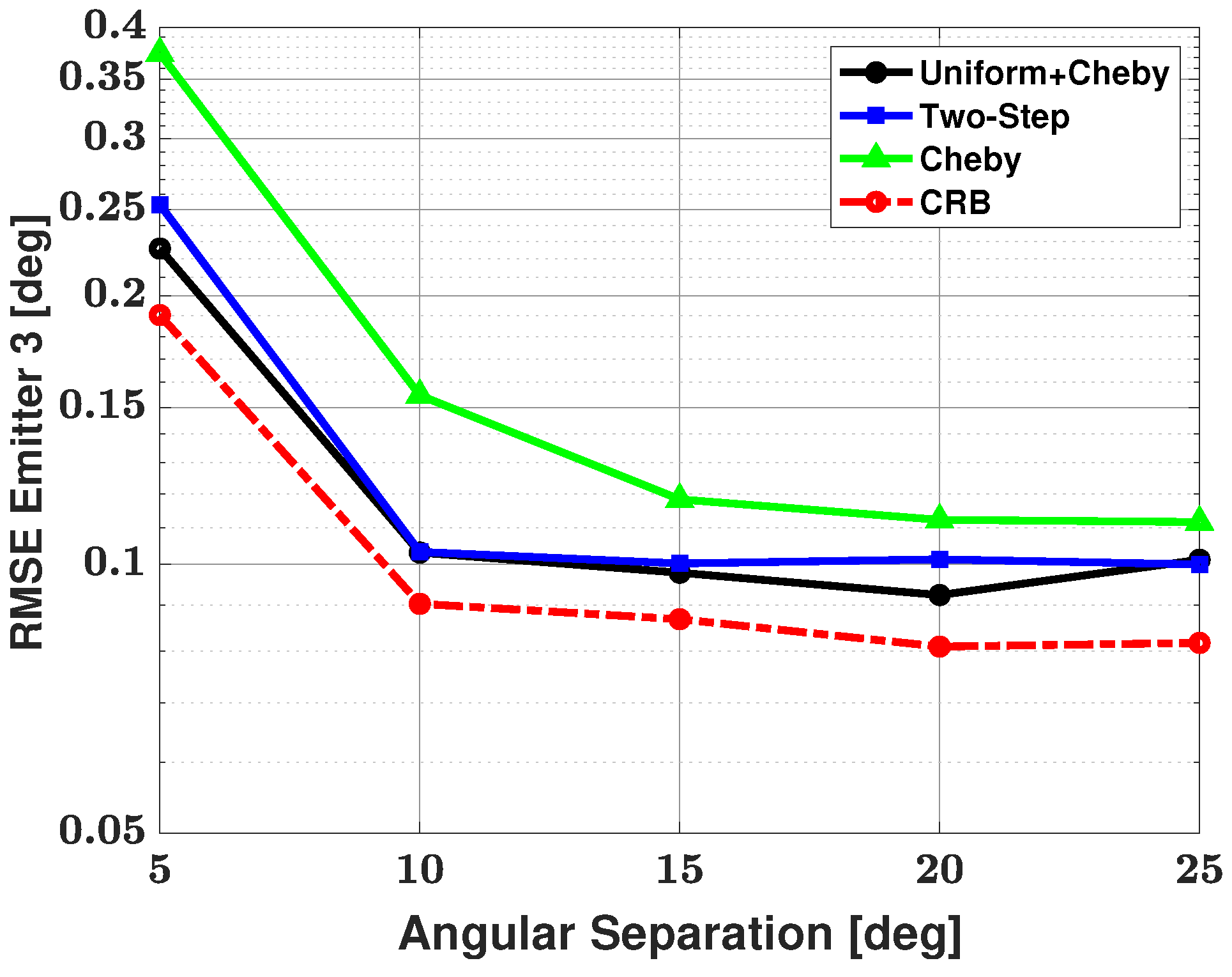
5.2. Three-Signal Scenario
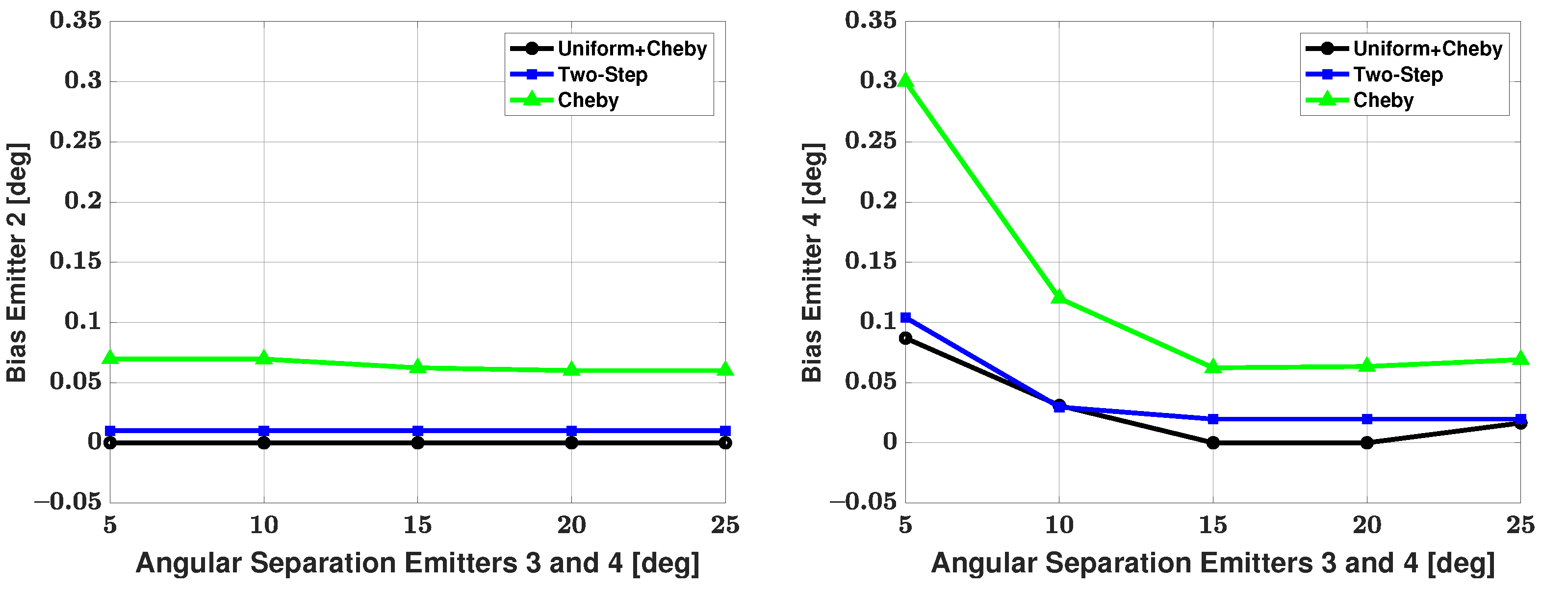
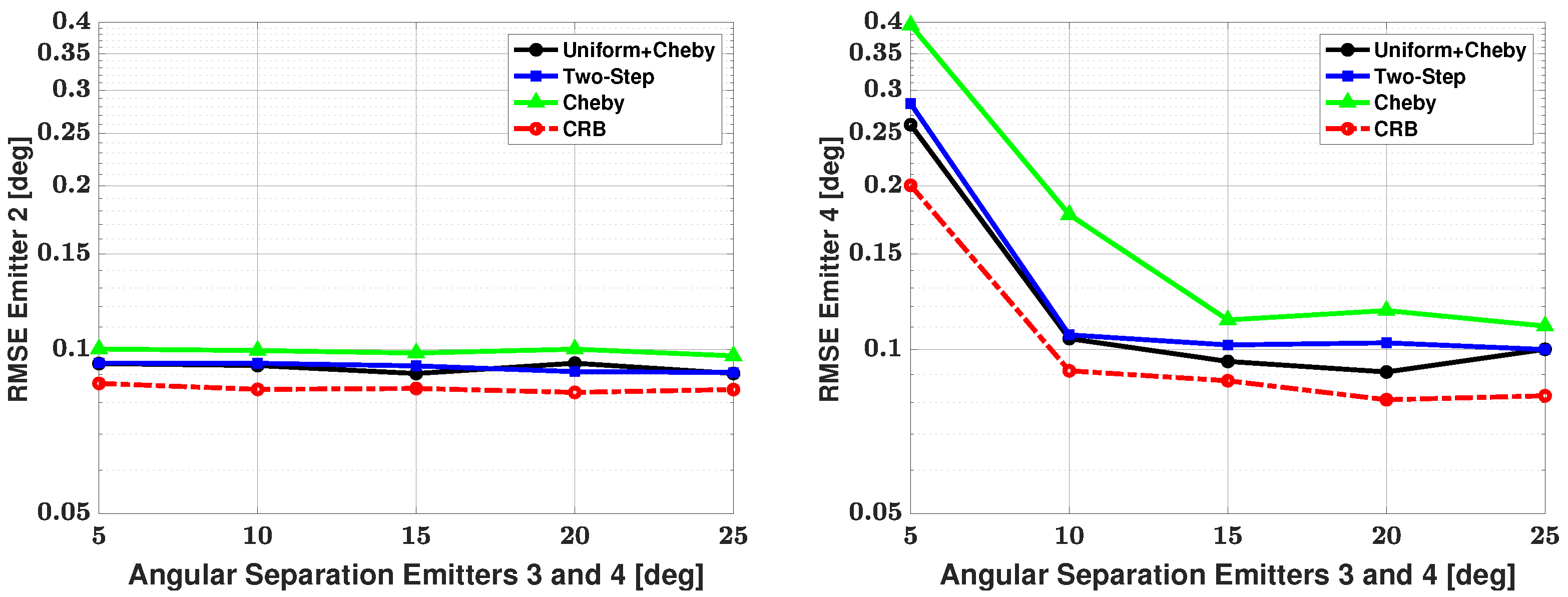
5.3. Four-Signal Scenario
6. Conclusions
Author Contributions
Funding
Institutional Review Board Statement
Informed Consent Statement
Data Availability Statement
Conflicts of Interest
References
- Bartlett, M.S. Smoothing Periodograms from Time-Series with Continuous Spectra. Nature 1948, 161, 686–687. [Google Scholar] [CrossRef]
- Schmidt, R. Multiple emitter location and signal parameter estimation. IEEE Trans. Antennas Propag. 1986, 34, 276–280. [Google Scholar] [CrossRef] [Green Version]
- Li, F.; Liu, H.; Vaccaro, R.J. Performance analysis for DOA estimation algorithms: Unification, simplification, and observations. IEEE Trans. Aerosp. Electron. Syst. 1993, 29, 1170–1184. [Google Scholar] [CrossRef]
- Hyder, M.M.; Mahata, K. Direction-of-Arrival Estimation Using a Mixed ℓ2,0 Norm Approximation. IEEE Trans. Signal Process. 2010, 58, 4646–4655. [Google Scholar] [CrossRef]
- Yin, J.; Chen, T. Direction-of-Arrival Estimation Using a Sparse Representation of Array Covariance Vectors. IEEE Trans. Signal Process. 2011, 59, 4489–4493. [Google Scholar] [CrossRef]
- Liu, Z.; Huang, Z.; Zhou, Y. Direction-of-Arrival Estimation of Wideband Signals via Covariance Matrix Sparse Representation. IEEE Trans. Signal Process. 2011, 59, 4256–4270. [Google Scholar] [CrossRef]
- Jisheng, D.; Zhen, W.; Zheng, T. Real-valued sparse representation method for DOA estimation with uniform linear array. In Proceedings of the 31st Chinese Control Conference, Hefei, China, 25–27 July 2012; pp. 3794–3797. [Google Scholar]
- Stoica, P.; Babu, P.; Li, J. SPICE: A Sparse Covariance-Based Estimation Method for Array Processing. IEEE Trans. Signal Process. 2011, 59, 629–638. [Google Scholar] [CrossRef]
- Xu, X.; Wei, X.; Ye, Z. DOA Estimation Based on Sparse Signal Recovery Utilizing Weighted l1-Norm Penalty. IEEE Signal Process. Lett. 2012, 19, 155–158. [Google Scholar] [CrossRef]
- Zhao, G.; Shi, G.; Shen, F.; Luo, X.; Niu, Y. A Sparse Representation-Based DOA Estimation Algorithm with Separable Observation Model. IEEE Antennas Wirel. Propag. Lett. 2015, 14, 1586–1589. [Google Scholar] [CrossRef]
- He, Z.Q.; Liu, Q.H.; Jin, L.N.; Ouyang, S. Low complexity method for DOA estimation using array covariance matrix sparse representation. Electron. Lett. 2013, 49, 228–230. [Google Scholar] [CrossRef]
- Cheng, Z.; Zhao, Y.; Zhu, Y.; Shui, P.; Li, H. Sparse representation based two-dimensional direction-of-arrival estimation method with L-shaped array. IET Radar, Sonar Navig. 2016, 10, 976–982. [Google Scholar] [CrossRef]
- Cui, W.; Qian, T.; Tian, J. Enhanced covariances matrix sparse representation method for DOA estimation. Electron. Lett. 2015, 51, 1288–1290. [Google Scholar] [CrossRef]
- Si, W.; Wang, Y.; Zhang, C. 2D-DOA and Polarization Estimation Using a Novel Sparse Representation of Covariance Matrix with COLD Array. IEEE Access 2018, 6, 66385–66395. [Google Scholar] [CrossRef]
- Cai, J.; Bao, D.; Li, P.; Cai, J.; Bao, D.; Li, P. DOA estimation via sparse recovering from the smoothed covariance vector. J. Syst. Eng. Electron. 2016, 27, 555–561. [Google Scholar] [CrossRef]
- Carlin, M.; Rocca, P.; Oliveri, G.; Viani, F.; Massa, A. Directions-of-Arrival Estimation Through Bayesian Compressive Sensing Strategies. IEEE Trans. Antennas Propag. 2013, 61, 3828–3838. [Google Scholar] [CrossRef]
- Wu, X.; Zhu, W.; Yan, J. Direction of Arrival Estimation for Off-Grid Signals Based on Sparse Bayesian Learning. IEEE Sensors J. 2016, 16, 2004–2016. [Google Scholar] [CrossRef]
- Dai, J.; Bao, X.; Xu, W.; Chang, C. Root Sparse Bayesian Learning for Off-Grid DOA Estimation. IEEE Signal Process. Lett. 2017, 24, 46–50. [Google Scholar] [CrossRef] [Green Version]
- Dai, J.; So, H.C. Sparse Bayesian Learning Approach for Outlier-Resistant Direction-of-Arrival Estimation. IEEE Trans. Signal Process. 2018, 66, 744–756. [Google Scholar] [CrossRef]
- Das, A. Real-Valued Sparse Bayesian Learning for Off-Grid Direction-of-Arrival (DOA) Estimation in Ocean Acoustics. IEEE J. Ocean. Eng. 2021, 46, 172–182. [Google Scholar] [CrossRef]
- Li, C.; Zhou, T.; Guo, Q.; Cui, H.-L. Compressive Beamforming Based on Multiconstraint Bayesian Framework. IEEE Trans. Geosci. Remote. Sens. 2021. [Google Scholar] [CrossRef]
- Pandey, R.; Nannuru, S.; Siripuram, A. Sparse Bayesian Learning for Acoustic Source Localization. In Proceedings of the ICASSP 2021—2021 IEEE International Conference on Acoustics, Speech and Signal Processing (ICASSP), Toronto, ON, Canada, 6–11 June 2021; pp. 4670–4674. [Google Scholar] [CrossRef]
- Shen, Q.; Liu, W.; Cui, W.; Wu, S. Underdetermined DOA Estimation Under the Compressive Sensing Framework: A Review. IEEE Access 2016, 4, 8865–8878. [Google Scholar] [CrossRef]
- Shi, J.; Hu, G.; Zhang, X.; Sun, F.; Zhou, H. Sparsity-Based Two-Dimensional DOA Estimation for Coprime Array: From Sum—Difference Coarray Viewpoint. IEEE Trans. Signal Process. 2017, 65, 5591–5604. [Google Scholar] [CrossRef]
- Shi, J.; Hu, G.; Zhang, X.; Sun, F.; Zheng, W.; Xiao, Y. Generalized Co-Prime MIMO Radar for DOA Estimation with Enhanced Degrees of Freedom. IEEE Sens. J. 2018, 18, 1203–1212. [Google Scholar] [CrossRef]
- Cheng, Z.; Zhao, Y.; Li, H.; Shui, P. Two-dimensional DOA estimation algorithm with co-prime array via sparse representation. Electron. Lett. 2015, 51, 2084–2086. [Google Scholar] [CrossRef]
- Li, J.; Li, Y.; Zhang, X. Two-Dimensional Off-Grid DOA Estimation Using Unfolded Parallel Coprime Array. IEEE Commun. Lett. 2018, 22, 2495–2498. [Google Scholar] [CrossRef]
- Shi, Y.; Mao, X.; Zhao, C.; Liu, Y. A Block Alternating Optimization Method for Direction-of-Arrival Estimation with Nested Array. IEEE Access 2019, 7, 76659–76668. [Google Scholar] [CrossRef]
- Huang, H.; Liao, B.; Guo, C.; Huang, J. Sparse representation based DOA estimation using a modified nested linear array. In Proceedings of the 2018 IEEE Radar Conference (RadarConf18), Oklahoma City, OK, USA, 23–27 April 2018. [Google Scholar]
- Huang, X.; Yang, X.; Cao, L.; Lu, W. Pseudo Noise Subspace based DOA Estimation for Unfolded Coprime Linear Arrays. IEEE Wirel. Commun. Lett. 2021. [Google Scholar] [CrossRef]
- Ibrahim, M.; Römer, F.; Alieiev, R.; Galdo, G.D.; Thomä, R.S. On the estimation of grid offsets in CS-based direction-of-arrival estimation. In Proceedings of the 22014 IEEE International Conference on Acoustics, Speech and Signal Processing (ICASSP), Florence, Italy, 4–9 May 2014; pp. 6776–6780. [Google Scholar]
- Pallotta, L.; Giunta, G.; Farina, A. DOA Refinement Through Complex Parabolic Interpolation of a Sparse Recovered Signal. IEEE Signal Process. Lett. 2021, 28, 274–278. [Google Scholar] [CrossRef]
- Zhang, X.; Jiang, T.; Li, Y.; Liu, X. An Off-Grid DOA Estimation Method Using Proximal Splitting and Successive Nonconvex Sparsity Approximation. IEEE Access 2019, 7, 66764–66773. [Google Scholar] [CrossRef]
- Compaleo, J.; Gupta, I.J. Application of Sparse Representation to Bartlett Spectra for Improved Direction of Arrival Estimation. Sensors 2021, 21, 77. [Google Scholar] [CrossRef]
- Fuchs, J. On the application of the global matched filter to DOA estimation with uniform circular arrays. IEEE Trans. Signal Process. 2001, 49, 702–709. [Google Scholar] [CrossRef]
- Liu, Q.; Zeng, C.; Li, S.; Yang, Z.; Liao, G. Robust estimations of DOA and source number with strong and weak signals coexisting simultaneously based on a sparse uniform array. J. Eng. 2019, 2019, 6387–6389. [Google Scholar] [CrossRef]
- Gao, Y.; Xu, J.; Jia, X.; Long, T. A novel joint method for source number and DOA estimation for closely spaced sources. In Proceedings of the 2015 IEEE China Summit and International Conference on Signal and Information Processing (ChinaSIP), Chengdu, China, 12–15 July 2015; pp. 128–131. [Google Scholar]
- Qu, J.; Li, X.; Wen, Y. A new method for weak signals’ DOA estimation in the presence of strong interferences. In Proceedings of the 2012 IEEE 11th International Conference on Signal Processing, Beijing, China, 21–25 October 2012; pp. 320–323. [Google Scholar]
- Stankwitz, H.C.; Dallaire, R.J.; Fienup, J.R. Spatially variant apodization for sidelobe control in SAR imagery. In Proceedings of the 1994 IEEE National Radar Conference, Atlanta, GA, USA, 29–31 March 1994; pp. 132–137. [Google Scholar]
- Stoica, P.; Nehorai, A. Performance study of conditional and unconditional direction-of-arrival estimation. IEEE Trans. Acoust. Speech Signal Process. 1990, 38, 1783–1795. [Google Scholar] [CrossRef]
- Besson, O.; Abramovich, Y.I. Regularized Covariance Matrix Estimation in Complex Elliptically Symmetric Distributions Using the Expected Likelihood Approach—Part 2: The Under-Sampled Case. IEEE Trans. Signal Process. 2013, 61, 5819–5829. [Google Scholar] [CrossRef] [Green Version]
- De Maio, A.; Pallotta, L.; Li, J.; Stoica, P. Loading Factor Estimation Under Affine Constraints on the Covariance Eigenvalues With Application to Radar Target Detection. IEEE Trans. Aerosp. Electron. Syst. 2019, 55, 1269–1283. [Google Scholar] [CrossRef]
- Steiner, M.; Gerlach, K. Fast converging adaptive processor or a structured covariance matrix. IEEE Trans. Aerosp. Electron. Syst. 2000, 36, 1115–1126. [Google Scholar] [CrossRef]
- Aubry, A.; Maio, A.D.; Pallotta, L. A Geometric Approach to Covariance Matrix Estimation and its Applications to Radar Problems. IEEE Trans. Signal Process. 2018, 66, 907–922. [Google Scholar] [CrossRef] [Green Version]
- Malioutov, D.; Cetin, M.; Willsky, A.S. A sparse signal reconstruction perspective for source localization with sensor arrays. IEEE Trans. Signal Process. 2005, 53, 3010–3022. [Google Scholar] [CrossRef] [Green Version]
- SeDuMi. Available online: http://sedumi.ie.lehigh.edu (accessed on 15 November 2018).
- Mallat, S.G.; Zhang, Z. Matching Pursuits with Time-Frequency Dictionaries. IEEE Trans. Signal Process. 1993, 41, 3397–3415. [Google Scholar] [CrossRef] [Green Version]
- Stoica, P.; Nehorai, A. MUSIC, maximum likelihood, and Cramer-Rao bound. IEEE Trans. Acoust. Speech Signal Process. 1989, 37, 720–741. [Google Scholar] [CrossRef]


| Angular Sep. [Deg] | Two-Step Approach | Uniform+Cheby | Cheby |
|---|---|---|---|
| 5 | 15 | 7 | 7 |
| 10 | 8 | 0 | 0 |
| 15 | 0 | 0 | 0 |
| 20 | 0 | 0 | 0 |
| 25 | 0 | 0 | 0 |
| Angular Sep. [deg] | Two-Step Approach | Uniform+Cheby | Cheby |
|---|---|---|---|
| 5 | 22 | 9 | 9 |
| 10 | 9 | 0 | 0 |
| 15 | 0 | 0 | 0 |
| 20 | 0 | 0 | 0 |
| 25 | 0 | 0 | 0 |
| Angular Sep. [deg] | Two-Step Approach | Uniform+Cheby | Cheby |
|---|---|---|---|
| 5 | 24 | 9 | 9 |
| 10 | 13 | 0 | 0 |
| 15 | 8 | 0 | 0 |
| 20 | 0 | 0 | 0 |
| 25 | 0 | 0 | 0 |
Publisher’s Note: MDPI stays neutral with regard to jurisdictional claims in published maps and institutional affiliations. |
© 2021 by the authors. Licensee MDPI, Basel, Switzerland. This article is an open access article distributed under the terms and conditions of the Creative Commons Attribution (CC BY) license (https://creativecommons.org/licenses/by/4.0/).
Share and Cite
Compaleo, J.; Gupta, I.J. Spectral Domain Sparse Representation for DOA Estimation of Signals with Large Dynamic Range. Sensors 2021, 21, 5164. https://doi.org/10.3390/s21155164
Compaleo J, Gupta IJ. Spectral Domain Sparse Representation for DOA Estimation of Signals with Large Dynamic Range. Sensors. 2021; 21(15):5164. https://doi.org/10.3390/s21155164
Chicago/Turabian StyleCompaleo, Jacob, and Inder J. Gupta. 2021. "Spectral Domain Sparse Representation for DOA Estimation of Signals with Large Dynamic Range" Sensors 21, no. 15: 5164. https://doi.org/10.3390/s21155164