
The Identification of the Uncertainty in Soil Strength Parameters Based on CPTu Measurements and Random Fields


Abstract
:1. Introduction
- Is it possible to identify stationary random fields only based on appropriately transformed CPT results?
- Do the variability and trends of selected strength parameters determined by CPT signal transformation behave similarly to the same values obtained from laboratory tests?
- Do any of the existing methods of estimation c′ and ϕ′ based on CPT provide reliable results for identifying random fields for these parameters, and do they also allow obtaining a reliable value for the cross-correlation coefficient between these fields?
2. Materials and Methods
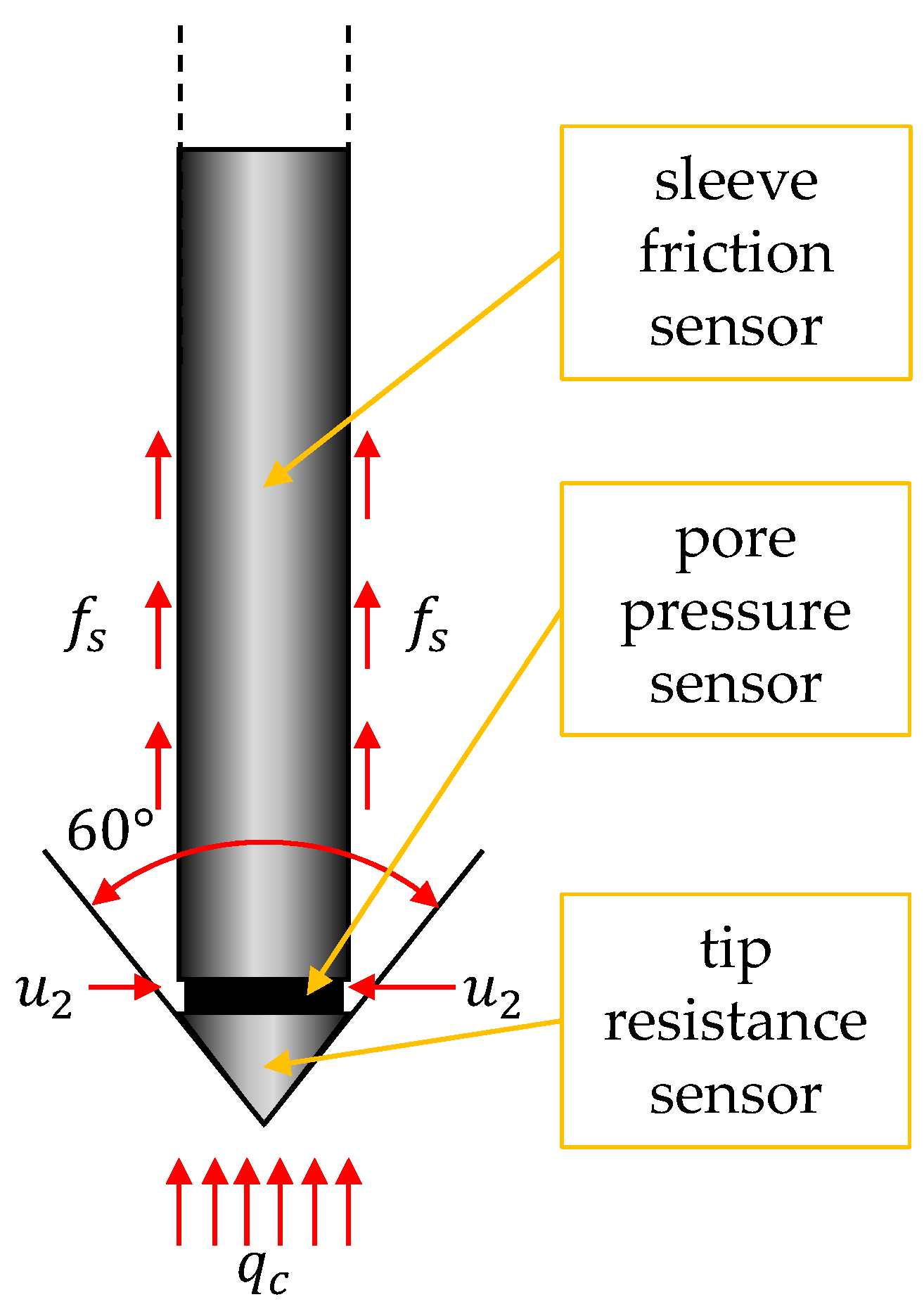
2.1. Method of Measurement
2.2. Methods of Interpretation of Strength Parameters Based on CPT Data
2.3. Method for Identification of Vertical SOF
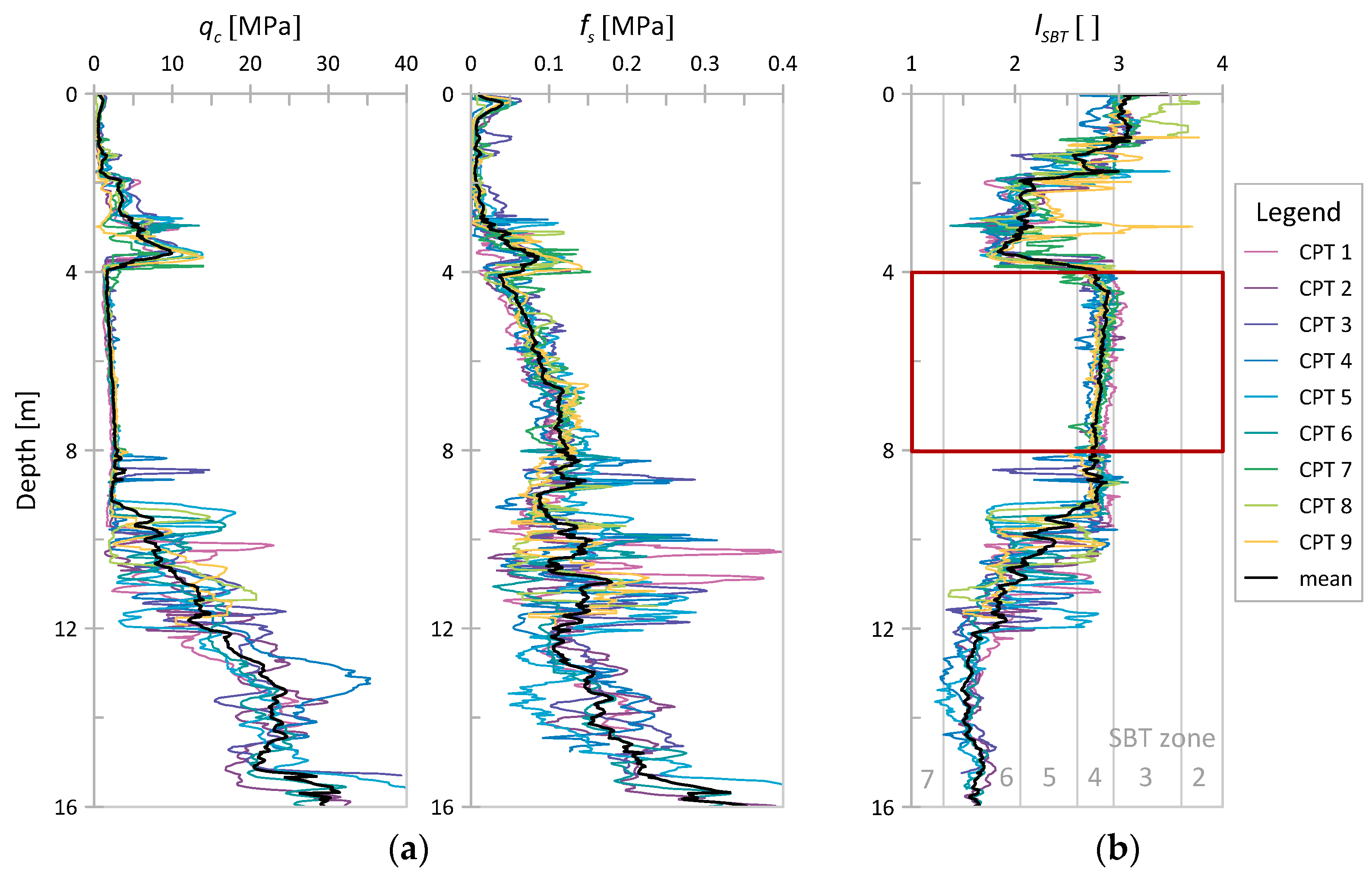
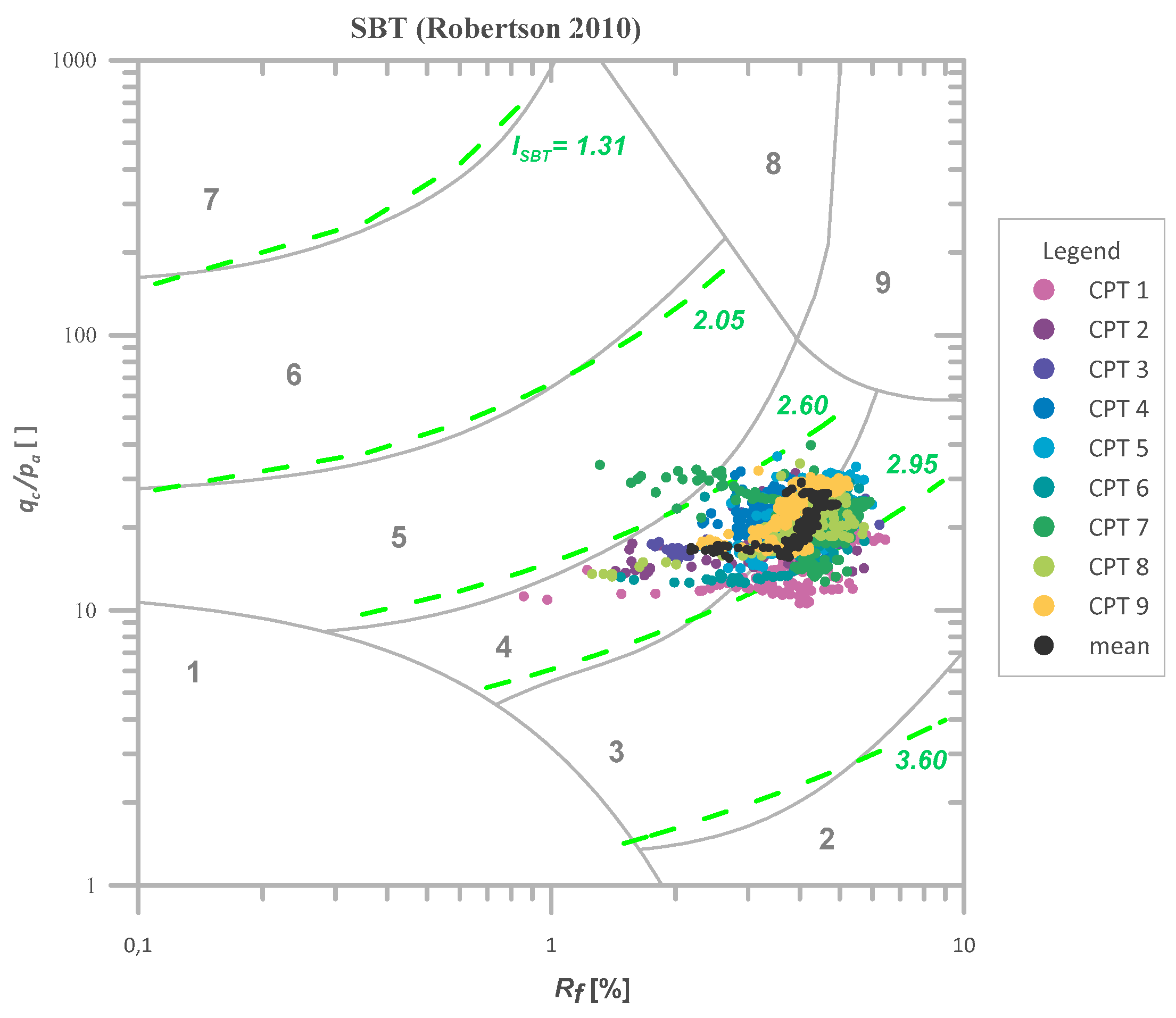
2.4. Materials–Sensing Data
2.5. Materials–Verification Data
3. Results
3.1. Determined Values of Undrained Shear Strength su
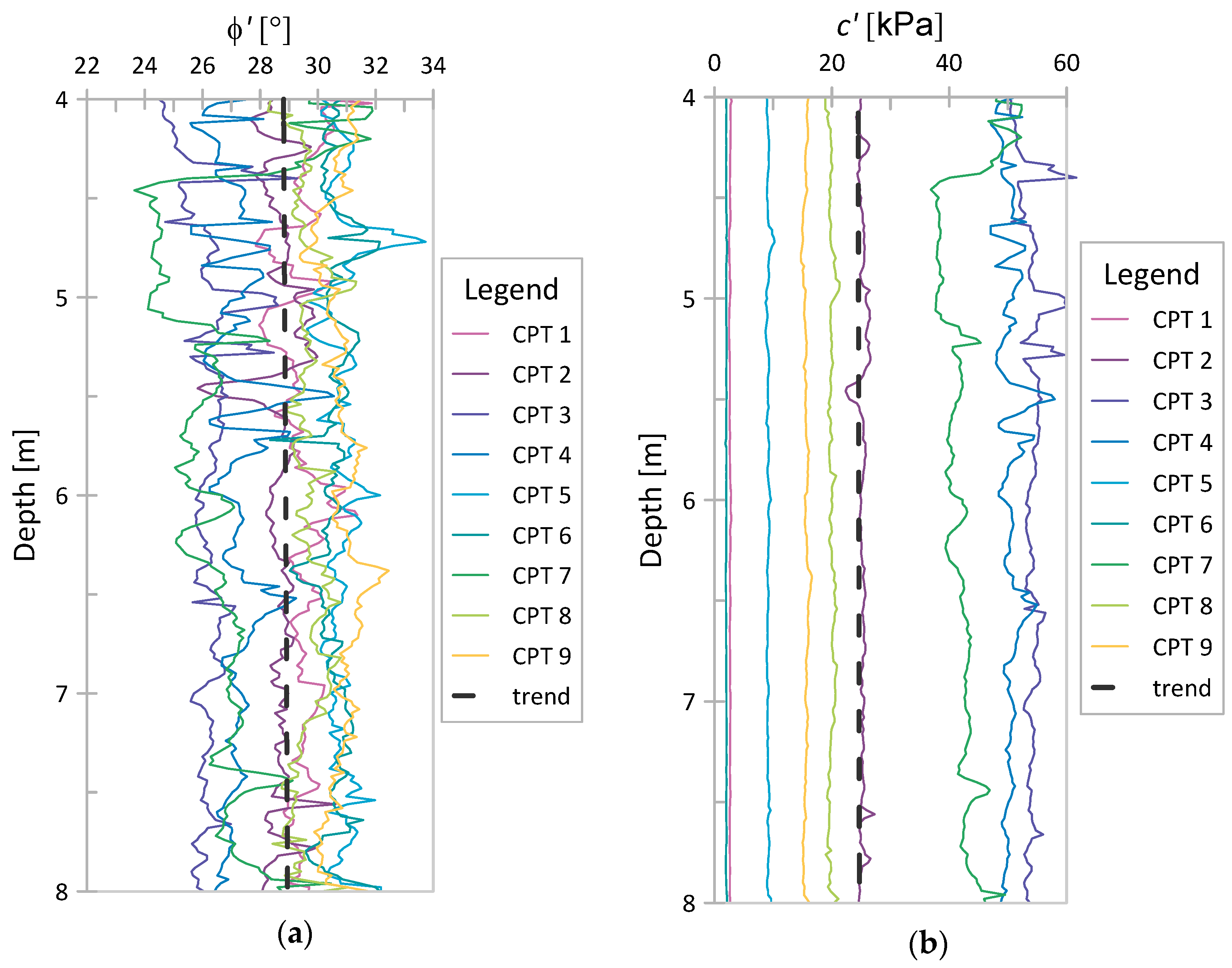
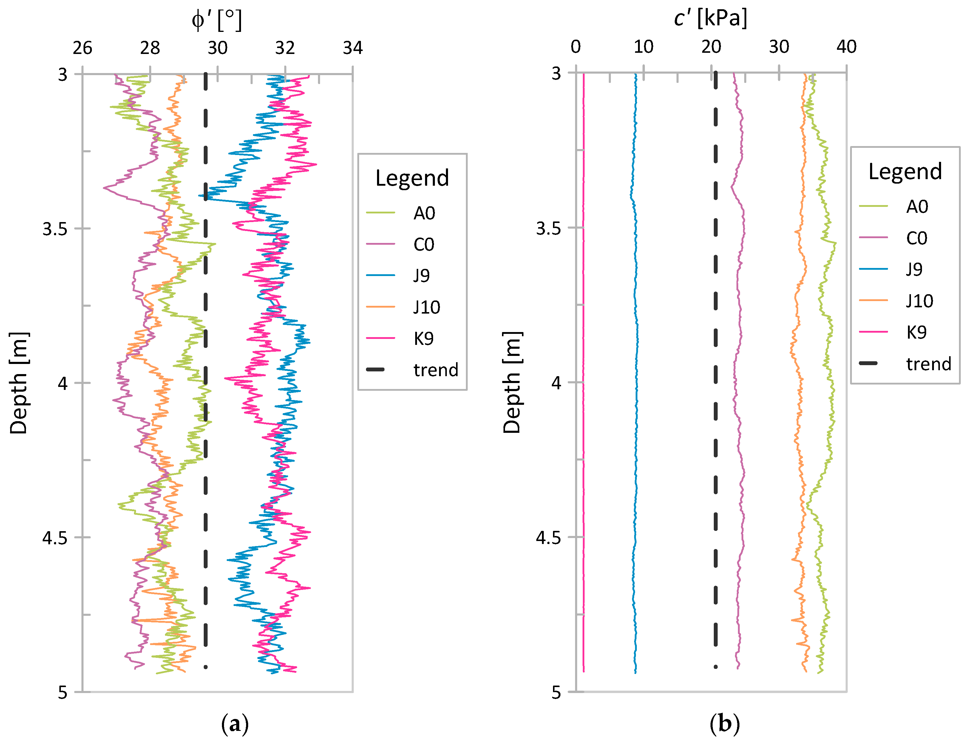
3.2. Shear Strength Parameters ϕ′ and c′ Determined by the NTH Method
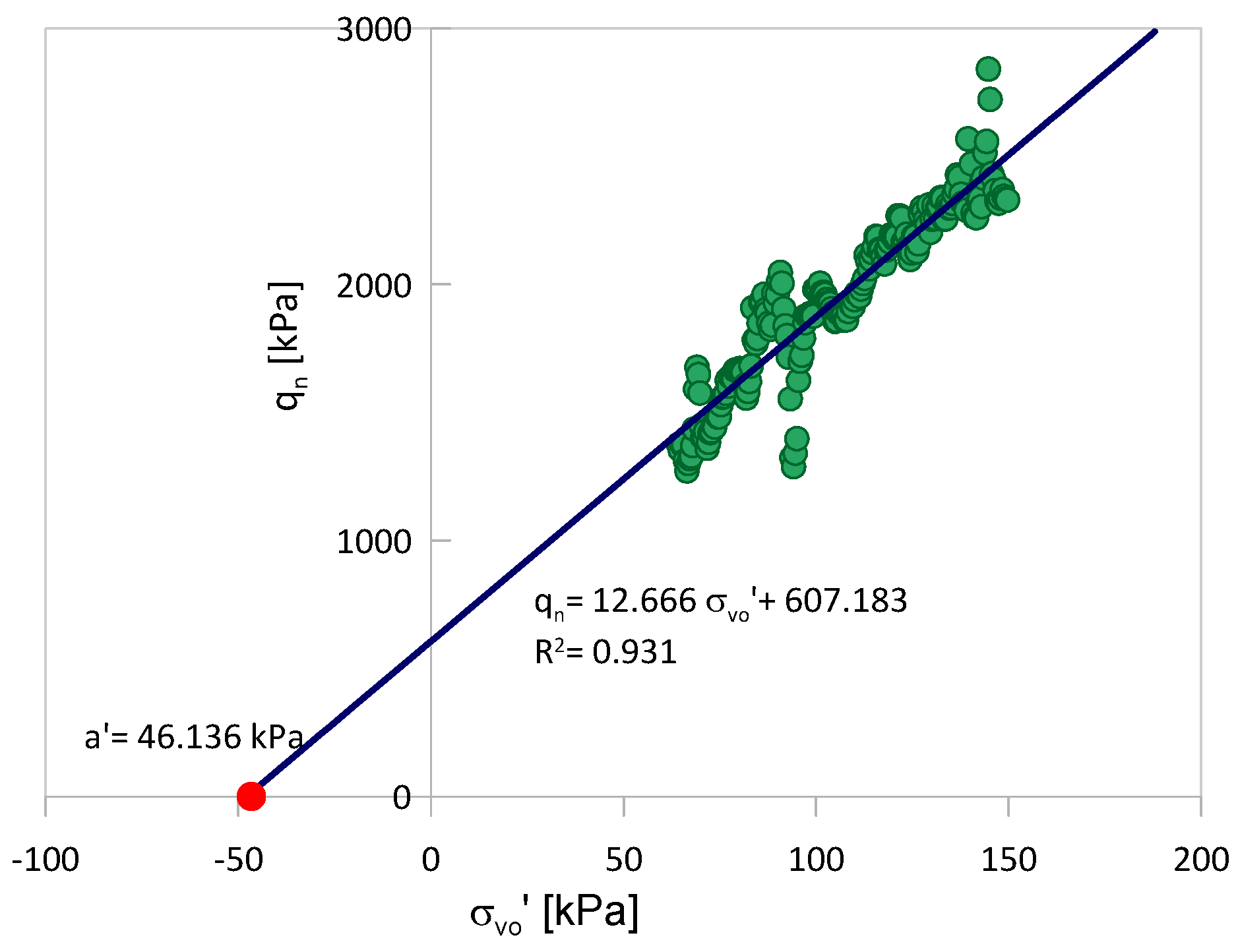
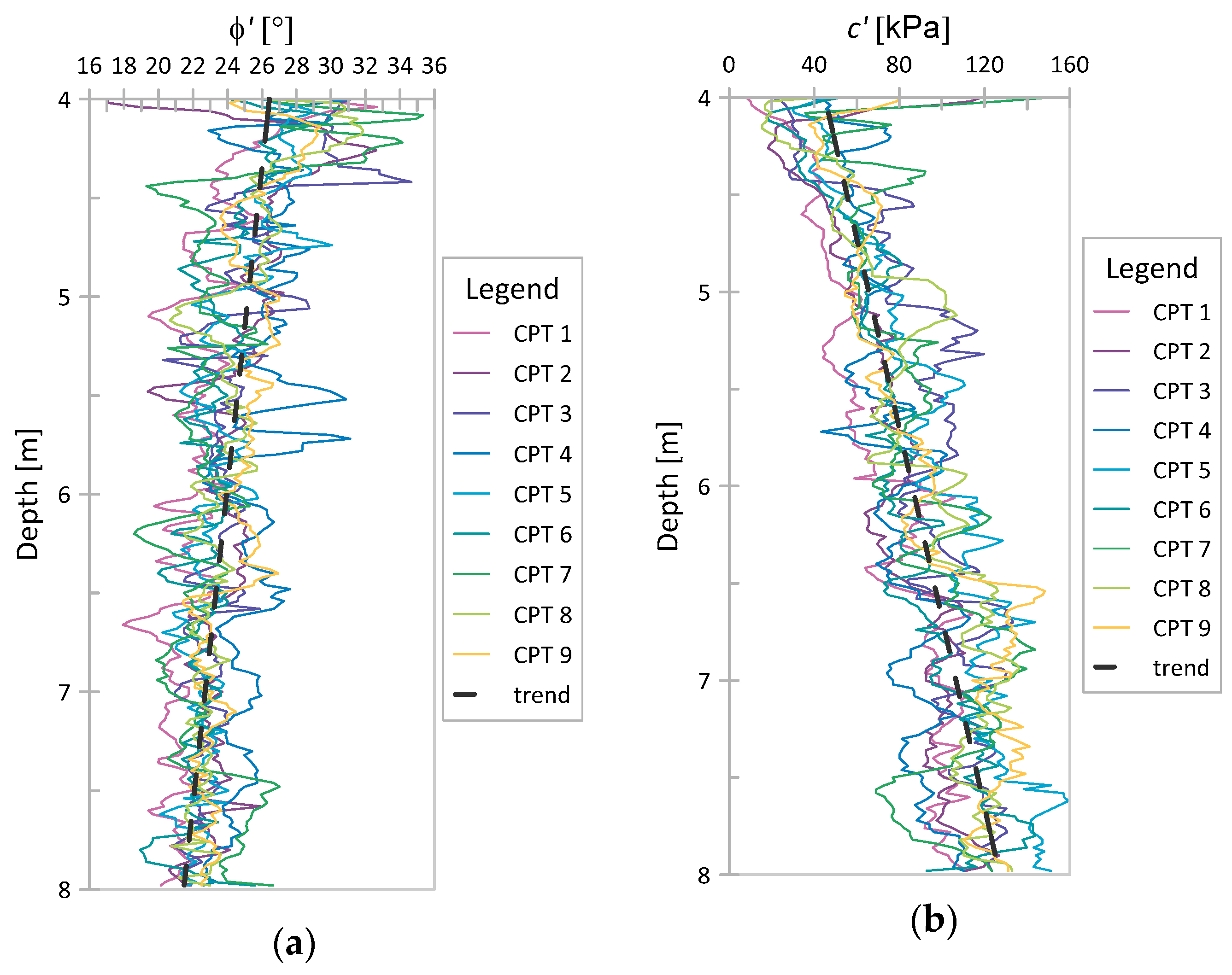
3.3. Shear Strength Parameters ϕ′ and c′ Determined by the Method of Equations
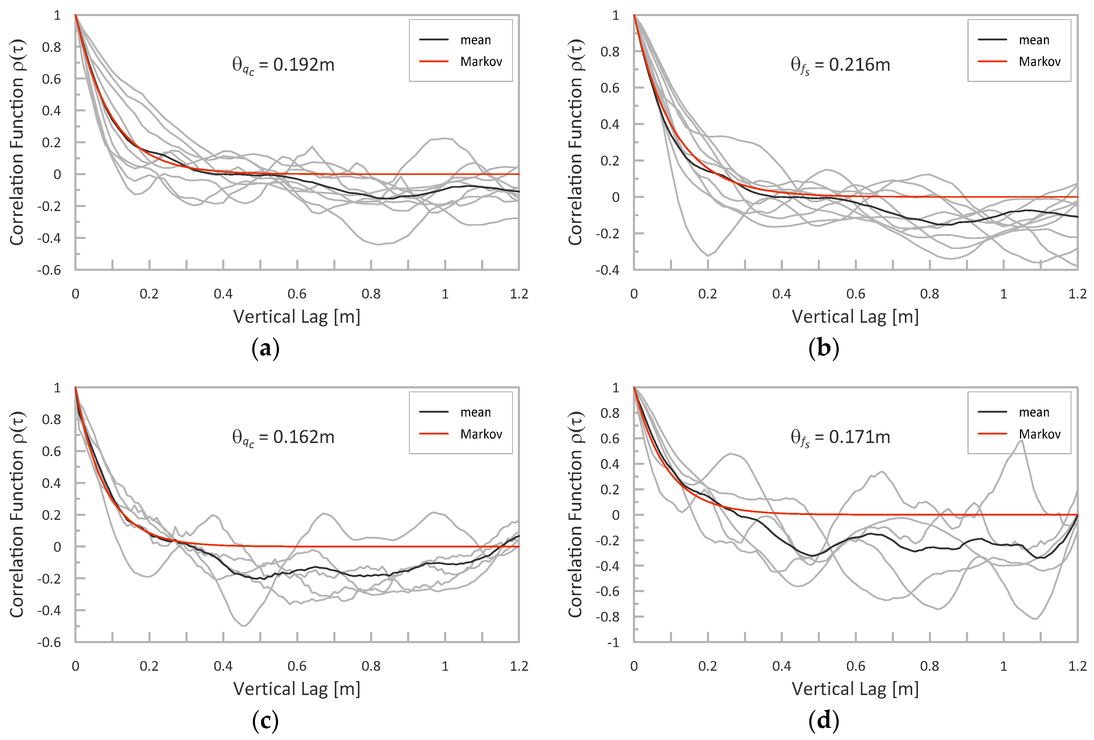
3.4. Vertical SOF
3.5. Cross-Correlation Coefficient ρ between c′and ϕ′
4. Discussion of Results
4.1. Variability in the Undrained Shear Strength su
4.2. Variability in ϕ′ and c′ Based on the NTH Method and MoE
4.3. Vertical Scale of Fluctuation for Original and Transformed Signals
4.4. Cross-Correlation Coefficient ρ
5. Conclusions
- The uncertainty of the model parameters is an essential issue, which once identified allows for managing specific resources. In numerical modeling of geotechnical structures, the problem can refer to the uncertainty in shear strength parameters. Understanding this uncertainty enables one to manage the risk of failure by designing the structure for the specific failure probability. While in typical numerical studies, the strength parameters of soils are modeled as constant, using SRF to describe this uncertainty is the approach with rising interest.
- When stationary random fields are used to model soil strength parameters, data from two different sources are typically used for their identification; the scale of fluctuation is assessed based on CPT and point statistics based on laboratory tests, which are often limited in number. More sophisticated statistical modeling approaches are based on large databases of both filed and laboratory test results, which are rarely available and associated with high costs. The proposed procedure allows for identifying the parameters of SRF for cohesive soil in the case of insufficient information regarding laboratory test results, based only on CPT measurements. Despite the relatively simple approach of analyzing the directly transformed CPT signal, the resulting measures of variability, which allow identifying the random SRF, appear to agree very well with the literature data.
- The presented procedure applied to the su parameter in Keswick clay (for which both laboratory and field test results were available) predicted a similar trend of su to that obtained based on laboratory tests. Although the COV value obtained based on those CPTs appeared to be slightly less than ten from laboratory tests, it remains in a reasonable range. Moreover, the COV values for the ϕ′ and c′ parameters as well as the cross-correlation coefficient ρ for these parameters (obtained using the NTH method) fall within the range of typical values obtained in laboratory investigations.
- The lack of strong trends of c′ and ϕ′ resulting from the NTH method confirmed by laboratory test results proves that modeling these parameters by stationary random fields (which is a common practice) is correct. However, that is not the case for su. The strong trend obtained for that parameter should be accounted for in its random field representation.
- The performed analysis shows that the fluctuation scale determined for qc or fs does not change when the obtained values are transformed to su, or ϕ′ and c′ (particularly in the case of the NTH method). As the transformations used are practically linear, it is not surprising. These results, however, are in line with the commonly used assumption that the fluctuation scales for different parameters should be equal.
- The value of c′ obtained using the method of equations significantly differs from the values obtained from the NTH method. It seems that the value of cohesion obtained with this method does not represent the effective value of cohesion c′, and the method probably needs to be further developed. The concept of the method is, however, very interesting and seems worthy of further investigation.
Author Contributions
Funding
Conflicts of Interest
References
- Orellana, R.; Carvajal, R.; Escárate, P.; Agüero, J.C. On the Uncertainty Identification for Linear Dynamic Systems Using Stochastic Embedding Approach with Gaussian Mixture Models. Sensors 2021, 21, 3837. [Google Scholar] [CrossRef]
- Segarra, E.L.; Ruiz, G.R.; Bandera, C.F. Probabilistic Load Forecasting Optimization for Building Energy Models via Day Characterization. Sensors 2021, 21, 3299. [Google Scholar] [CrossRef] [PubMed]
- Vanmarcke, E. Random Fields: Analysis and Synthesis; MIT Press: Cambridge, MA, USA, 1983. [Google Scholar]
- Fenton, G.A.; Griffiths, D.V. Bearing-capacity prediction of spatially random c–ϕ soils. Can. Geotech. J. 2003, 40, 54–65. [Google Scholar] [CrossRef]
- Griffiths, D.V.; Fenton, G.A. Bearing capacity of spatially random soil: The undrained clay Prandtl problem revisited. Géotechnique 2001, 51, 351–359. [Google Scholar] [CrossRef]
- Hicks, M.A.; Nuttall, J.D.; Chen, J. Influence of heterogeneity on 3D slope reliability and failure consequence. Comput. Geotech. 2014, 61, 198–208. [Google Scholar] [CrossRef]
- Pieczynska-Kozlowska, J.M.; Puła, W.; Griffiths, D.V.; Fenton, G.A. Influence of embedment, self-weight and anisotropy on bearing capacity reliability using the random finite element method. Comput. Geotech. 2015, 67, 229–238. [Google Scholar] [CrossRef]
- Vessia, G.; Kozubal, J.; Puła, W. High dimensional model representation for reliability analyses of complex rock–soil slope stability. Arch. Civ. Mech. Eng. 2017, 17, 954–963. [Google Scholar] [CrossRef]
- Kawa, M.; Puła, W. 3D bearing capacity probabilistic analyses of footings on spatially variable c–φ soil. Acta Geotech. 2019, 15, 1453–1466. [Google Scholar] [CrossRef] [Green Version]
- Kawa, M.; Baginska, I.; Wyjadlowski, M. Reliability analysis of sheet pile wall in spatially variable soil including CPTu test results. Arch. Civ. Mech. Eng. 2019, 19, 598–613. [Google Scholar] [CrossRef]
- Puła, W. On some aspects of reliability computations in bearing capacity of shallow foundations. In Probabilistic Methods in Geotechnical Engineering; Springer: Vienna, Austria, 2007; pp. 127–145. [Google Scholar]
- Ching, J.; Phoon, K.-K. Constructing Site-Specific Multivariate Probability Distribution Model Using Bayesian Machine Learning. J. Eng. Mech. 2019, 145, 04018126. [Google Scholar] [CrossRef]
- Sert, S.; Luo, Z.; Xiao, J.; Gong, W.; Juang, C.H. Probabilistic analysis of responses of cantilever wall-supported excavations in sands considering vertical spatial variability. Comput. Geotech. 2016, 75, 182–191. [Google Scholar] [CrossRef]
- Chwała, M. Undrained bearing capacity of spatially random soil for rectangular footings. Soils Found. 2019, 59, 1508–1521. [Google Scholar] [CrossRef]
- Xiao, T.; Li, D.-Q.; Cao, Z.-J.; Zhang, L.-M. CPT-Based Probabilistic Characterization of Three-Dimensional Spatial Variability Using MLE. J. Geotech. Geoenviron. Eng. 2018, 144, 04018023. [Google Scholar] [CrossRef]
- Uzielli, M.; Mayne, P.W. Probabilistic assignment of effective friction angles of sands and silty sands from CPT using quantile regression. Georisk Assess. Manag. Risk Eng. Syst. Geohazards 2019, 13, 271–275. [Google Scholar] [CrossRef]
- Lloret-Cabot, M.; Fenton, G.A.; Hicks, M.A. On the estimation of scale of fluctuation in geostatistics. Georisk Assess. Manag. Risk Eng. Syst. Geohazards 2014, 8, 129–140. [Google Scholar] [CrossRef] [Green Version]
- Cafaro, F.; Cherubini, C. Large Sample Spacing in Evaluation of Vertical Strength Variability of Clayey Soil. J. Geotech. Geoenviron. Eng. 2002, 128, 558–568. [Google Scholar] [CrossRef]
- Jaksa, M.B.; Kaggwa, W.S.; Brooker, P.I. Experimental evaluation of the scale of fluctuation of a stiff clay. In Proceedings of the 8th International Conference on the Application of Statistics and Probability, Sydney, Australia, 12–15 December 1999; Volume 1, pp. 415–422. [Google Scholar]
- Pieczyńska-Kozłowska, J.M. Comparison between Two Methods for Estimating the Vertical Scale of Fluctuation for Modeling Random Geotechnical Problems. Stud. Geotech. Mech. 2015, 37, 95–103. [Google Scholar] [CrossRef] [Green Version]
- Wang, Y.; Zhao, T.; Hu, Y.; Phoon, K.-K. Simulation of Random Fields with Trend from Sparse Measurements without Detrending. J. Eng. Mech. 2019, 145, 04018130. [Google Scholar] [CrossRef]
- Ching, J.; Phoon, K.-K. Correlations among some clay parameters—The multivariate distribution. Can. Geotech. J. 2014, 51, 686–704. [Google Scholar] [CrossRef]
- Cami, B.; Javankhoshdel, S.; Phoon, K.-K.; Ching, J. Scale of Fluctuation for Spatially Varying Soils: Estimation Methods and Values. ASCE-ASME J. Risk Uncertain. Eng. Syst. Part A Civ. Eng. 2020, 6, 03120002. [Google Scholar] [CrossRef]
- Lunne, T.; Robertson, P.K.; Powell, J.J.M. Cone Penetration Testing in Geotechnical Practice; Blackie Academic/Routledge Publishing: New York, NY, USA, 1997. [Google Scholar]
- Stacul, S.; Magalotti, A.; Baglione, M.; Meisina, C.; Presti, D.L. Implementation and Use of a Mechanical Cone Penetration Test Database for Liquefaction Hazard Assessment of the Coastal Area of the Tuscany Region. Geosciences 2020, 10, 128. [Google Scholar] [CrossRef] [Green Version]
- EN ISO 22476-12:2009 Geotechnical Investigation and Testing—Field Testing—Part 12: Mechanical Cone Penetration Test (CPTM); International Organization for Standardization: Geneva, Switzerland, 2009.
- EN ISO 22476-1:2012 Geotechnical Investigation and Testing—Field Testing—Part 1: Electrical Cone and Piezocone Penetration Test; International Organization for Standardization: Geneva, Switzerland, 2012.
- Mayne, P.W. NCHRP Synthesis 368, Cone Penetration Testing; Transportation Research Board: Washington, DC, USA, 2007. [Google Scholar]
- Schneider, J.A.; Hoyos, L., Jr.; Mayne, P.W.; Macari, E.J.; Rix, G.J. Field and Laboratory Measurements of Dynamic Shear Modulus of Piedmont Residual Soils, Behavioral Characteristics of Residual Soils, GSP 92; ASCE: Reston, VA, USA, 1999; pp. 12–25. [Google Scholar]
- Bagińska, I.; Janecki, W.; Sobótka, M. On the interpretation of seismic cone penetration test (SCPT) results. Stud. Geotech. Mech. 2013, 35, 3–11. [Google Scholar] [CrossRef]
- Zheng, J.; Hryciw, R.D. Optical flow analysis of internal erosion and soil piping in images captured by the VisCPT. In Tunneling and Underground Construction; ASCE: Reston, VA, USA, 2014; pp. 55–64. [Google Scholar]
- Skutnik, Z.; Bajda, M.; Lech, M. Applications of RCPTU and SCPTU with other geophysical test methods in geotechnical practice. In Cone Penetration Testing 2018; CRC Press: Boca Raton, FL, USA, 2018; pp. 579–584. [Google Scholar]
- Cai, G.; Chu, Y.; Liu, S.; Puppala, A.J. Evaluation of subsurface spatial variability in site characterization based on RCPTU data. Bull. Int. Assoc. Eng. Geol. 2015, 75, 401–412. [Google Scholar] [CrossRef]
- Lunne, T.; Kleven, A. Role of CPT in North Sea foundation engineering. In Proceedings of Geotechniical Engineering, Division Session; ASCE National Convention: St. Louis, MO, USA, 1981; pp. 76–107. [Google Scholar]
- Robertson, P.K.; Cabal, K.L. Guide to Cone Penetration Testing For Geotechnical Engineering; Gregg Drilling & Testing: Signal Hill, CA, USA, 2015. [Google Scholar]
- Bagińska, I. Estimating and verifying soil unit weight determined on the basis of SCPTu tests. Ann. Wars. Univ. Life Sci. SGGW Land Reclam. 2016, 48, 233–242. [Google Scholar] [CrossRef] [Green Version]
- Senneset, K.; Janbu, N. Shear Strength Parameters Obtained from Static Cone Penetration Tests. In Strength Testing of Marine Sediments: Laboratory and In-Situ Measurements; ASTM International: West Conshohocken, PA, USA, 2008; p. 41. [Google Scholar]
- Motaghedi, H.; Armaghani, D.J. New method for estimation of soil shear strength parameters using results of piezocone. Measurement 2016, 77, 132–142. [Google Scholar] [CrossRef]
- Eslami, A.; Fellenius, B.H. Pile capacity by direct CPT and CPTu methods applied to 102 case histories. Can. Geotech. J. 1997, 34, 886–904. [Google Scholar] [CrossRef]
- Jamiokowski, M.; Robertson, P.K. Closing Address: Future Trends for Penetration Testing, Geotechnology Conference Pene-tration Testing in UK. In Proceedings of the Geotechnology Conference Organized by the Institution of Civil Engineers, Birmingham, UK, 6–8 July 1988; pp. 321–342. [Google Scholar]
- Mayne, P.W. Evaluating effective stress parameters and undrained shear strengths of soft-firm clays from CPT and DMT. Aust. Geomech. J. 2016, 51, 27–55. [Google Scholar]
- Puła, W.; Bagińska, I.; Kawa, M.; Pieczyńska-Kozłowska, J.M. Estimation of spatial variability of soil properties using CPTU results: A case study. In Proceedings of the 6th International Workshop: In Situ and Laboratory Characterization of OC Subsoil, Poznań, Poland, 26–27 June 2017; pp. 23–32. [Google Scholar]
- Jaksa, M.B. The Influence of Spatial Variability on the Geotechnical Design Properties of a Stiff, Overconsolidated Clay. Ph.D. Thesis, The University of Adelaide, Adelaide, Australia, 1995. Available online: http://hdl.handle.net/2440/37800 (accessed on 9 August 2021).
- Robertson, P.K. Soil behaviour type from the CPT: An update. In Proceedings of the 2nd International Symposium on Cone Penetration Testing, Huntington Beach, CA, USA, 9–11 May 2010. [Google Scholar]
- Greco, V.R. Variability and Correlation of Strength Parameters Inferred from Direct Shear Tests. Geotech. Geol. Eng. 2015, 34, 585–603. [Google Scholar] [CrossRef]
- Šujan, M.; Slávik, I.; Galliková, Z.; Dovičin, P.; Šujan, M. Pre-Quaternary basement of Bratislava (part 1): Genetic vs geotech-nical characteristics of the Neogene foundation soils. Acta Geol. Slovaca 2016, 8, 71–86. [Google Scholar]
- Sevaldson, R.A. The Slide in Lodalen, October 6th, 1954. Géotechnique 1956, 6, 167–182. [Google Scholar] [CrossRef]
- Wolff, T.F.; Hassan, A.; Khan, R.; Ur-Rasul, I.; Miller, M. Geotechnical Reliability of Dam and Levee Embankments; ERDC. GSL CR-04-01; US Army Engineer Research and Development Center: Vicksburg, MS, USA, 2004.
- Hata, Y.; Ichii, K.; Tokida, K.-I. A probabilistic evaluation of the size of earthquake induced slope failure for an embankment. Georisk Assess. Manag. Risk Eng. Syst. Geohazards 2012, 6, 73–88. [Google Scholar] [CrossRef]
- Di Matteo, L.; Valigi, D.; Ricco, R. Laboratory shear strength parameters of cohesive soils: Variability and potential effects on slope stability. Bull. Int. Assoc. Eng. Geol. 2013, 72, 101–106. [Google Scholar] [CrossRef]
- Li, D.-Q.; Qi, X.-H.; Cao, Z.-J.; Tang, X.-S.; Zhou, W.; Phoon, K.-K.; Zhou, C.-B. Reliability analysis of strip footing considering spatially variable undrained shear strength that linearly increases with depth. Soils Found. 2015, 55, 866–880. [Google Scholar] [CrossRef] [Green Version]


| Soil | Unit Weight [kN/m3] | IP [%] | OCR [-] |
|---|---|---|---|
| Świerzna clay | 22.02 ± 0.39 (from laboratory test) | 19.2 ± 2.3 (from laboratory test) | 6.77 ± 0.61 (from CPT korelation) |
| Keswick clay | 18 (Jaksa PhD [44]) | 25–88 (Jaksa PhD [44]) | 7.64 ± 0.33 (from CPT korelation) |
| Soil | Triaxial Test Type | No. of Samples (up to 10 m Depth) | Trends Equation [kPa] | Depth z [m] | COV [-] |
|---|---|---|---|---|---|
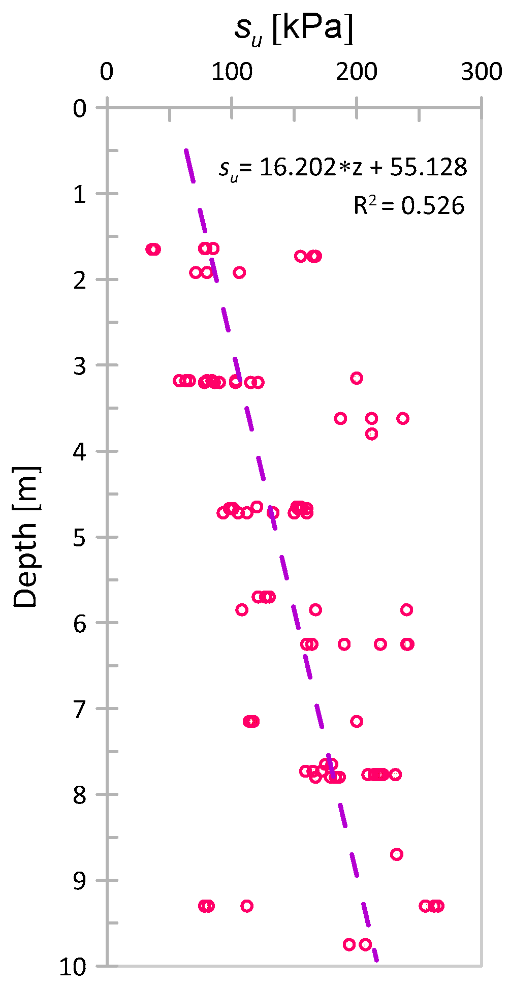
| Overconsolidated clay (Keswick clay) | UU and CU | 75 UU and 12 CU | su = 16.202 z + 55.128 | 3.2 | 0.33 |
| 4.7 | 0.19 | ||||
| 7.7 | 0.13 |
| Reference | Soil Type | Test Type | No. of Samples | COV for ϕ′ | COV for c′ | Parsons Coeff. Ρ | |
|---|---|---|---|---|---|---|---|
| Sevaldson [47] | Lightly overconsolidated clay (Lodalen landslide) | Triaxial CD | 10 | 0.060 | 0.210 | −0.070 | |
| Wolff et al. [48] | Bois Brule Levee embankment and foundation clay | Triaxial CD | 9 | 0.099–0.0165 | 1.280–1.310 | −0.388–−0.694 | |
| Hata et al. [49] | The cohesive soil-forming subsoil of Airports in Japan | APIII | Triaxial | 14CU | 0.192 | 1.068 | - |
| APIX | 14CU | 0.105 | 0.880 | - | |||
| APX | 10CD | 0.115 | 0.958 | −0.557 | |||
| Di Matteo et al. [50] | Silty clay | Direct shear | 16 | 0.030 | 0.210 | −0.925 | |
| Soil | Trends Equation [kPa] | Range of COV Values [-] | Mean COV [-] |
|---|---|---|---|
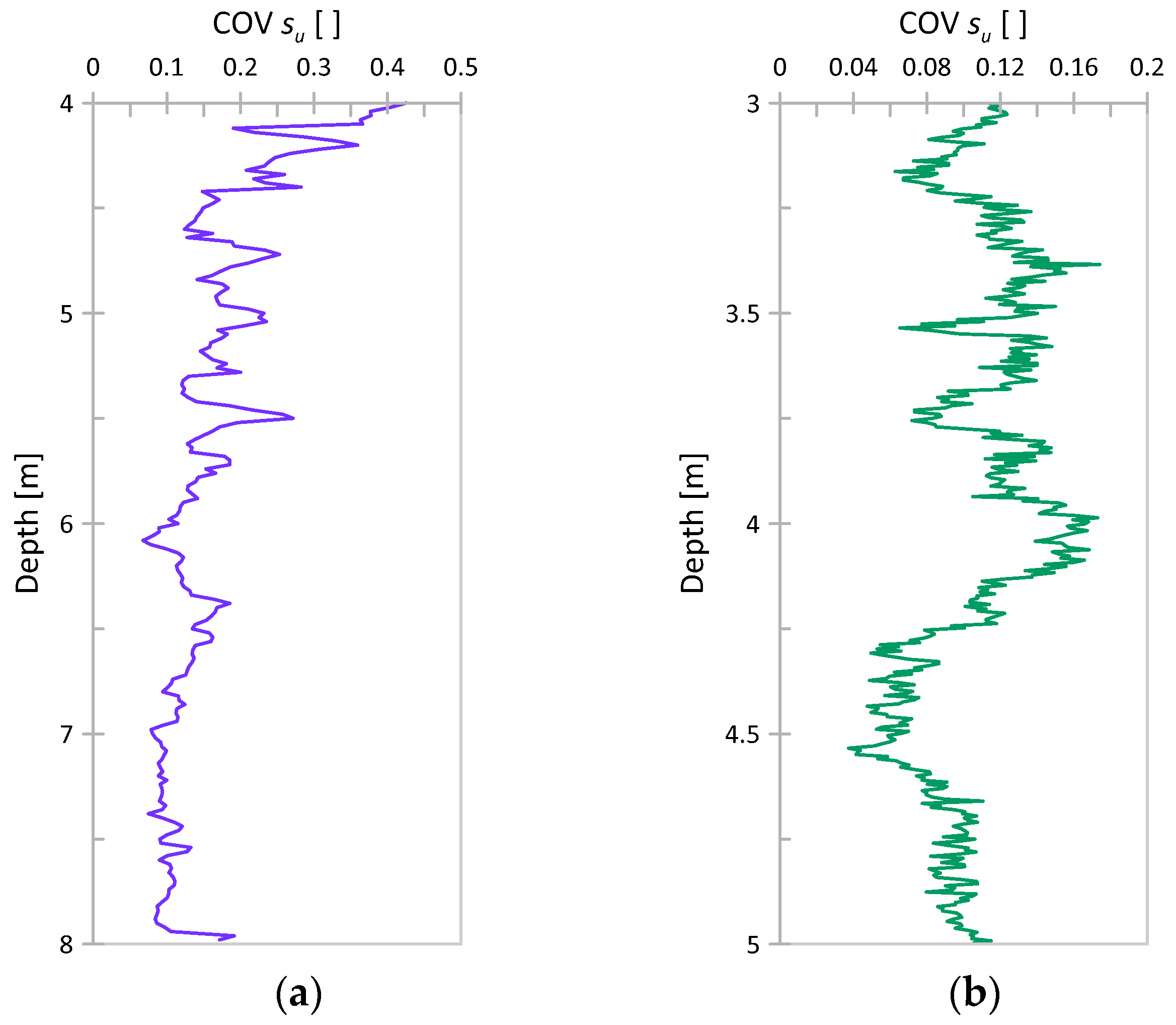
| Swierzna clay | su = 19.407 z + 19.539 | 0.068–0.425 | 0.152 |
| Keswick clay | su = 22.495 z + 30.620 | 0.038–0.186 | 0.105 |
| Global Value (All CPTs) | CPT1 | CPT2 | CPT3 | CPT4 | CPT5 | CPT6 | CPT7 | CPT8 | CPT9 | |
|---|---|---|---|---|---|---|---|---|---|---|
| Świerzna Clay a′ [kPa] | 44.19 | 4.7 | 46.1 | 110.0 | 98.2 | 15.3 | 3.4 | 84.2 | 35.1 | 26.2 |
| Keswick clay a′ [kPa] | 33.05 | CPTA0 | CPTC0 | CPTJ10 | CPTJ9 | CPTK9 | ||||
| 66.7 | 45.8 | 14.2 | 61.3 | 1.8 | ||||||
| ϕ′ | c′ | |||
|---|---|---|---|---|
| Mean [°] | COV [-] | Mean [°] | COV [-] | |
| Świerzna clay | 28.88 | 0.066 | 24.60 | 0.767 |
| Keswick clay | 29.64 | 0.058 | 20.65 | 0.663 |
| ϕ′ | c′ | |||
|---|---|---|---|---|
| Mean [°] | COV [-] | Mean [°] | COV [-] | |
| Świerzna clay | 23.95 | 0.103 | 85.90 | 0.339 |
| Keswick clay | 16.12 | 0.127 | 127.16 | 0.161 |
| Case Study | The Scale of Fluctuation (m) | ||||||
|---|---|---|---|---|---|---|---|
| Directly Measured by CPT | Undrained | Drained, MoE | Drained, NTH Method | ||||
| qc | fs | su | ϕ′ | c′ | ϕ′ | c′ | |
| Świerzna clay | 0.192 | 0.216 | 0.184 | 0.183 | 0.214 | 0.189 | 0.188 |
| Keswick clay | 0.162 | 0.171 | 0.166 | 0.121 | 0.166 | 0.164 | 0.164 |
Publisher’s Note: MDPI stays neutral with regard to jurisdictional claims in published maps and institutional affiliations. |
© 2021 by the authors. Licensee MDPI, Basel, Switzerland. This article is an open access article distributed under the terms and conditions of the Creative Commons Attribution (CC BY) license (https://creativecommons.org/licenses/by/4.0/).
Share and Cite
Pieczyńska-Kozłowska, J.; Bagińska, I.; Kawa, M. The Identification of the Uncertainty in Soil Strength Parameters Based on CPTu Measurements and Random Fields. Sensors 2021, 21, 5393. https://doi.org/10.3390/s21165393
Pieczyńska-Kozłowska J, Bagińska I, Kawa M. The Identification of the Uncertainty in Soil Strength Parameters Based on CPTu Measurements and Random Fields. Sensors. 2021; 21(16):5393. https://doi.org/10.3390/s21165393
Chicago/Turabian StylePieczyńska-Kozłowska, Joanna, Irena Bagińska, and Marek Kawa. 2021. "The Identification of the Uncertainty in Soil Strength Parameters Based on CPTu Measurements and Random Fields" Sensors 21, no. 16: 5393. https://doi.org/10.3390/s21165393