
New Radiometric Approaches to Compute Underwater Irradiances: Potential Applications for High-Resolution and Citizen Science-Based Water Quality Monitoring Programs


Abstract
1. Introduction
2. Materials and Methods
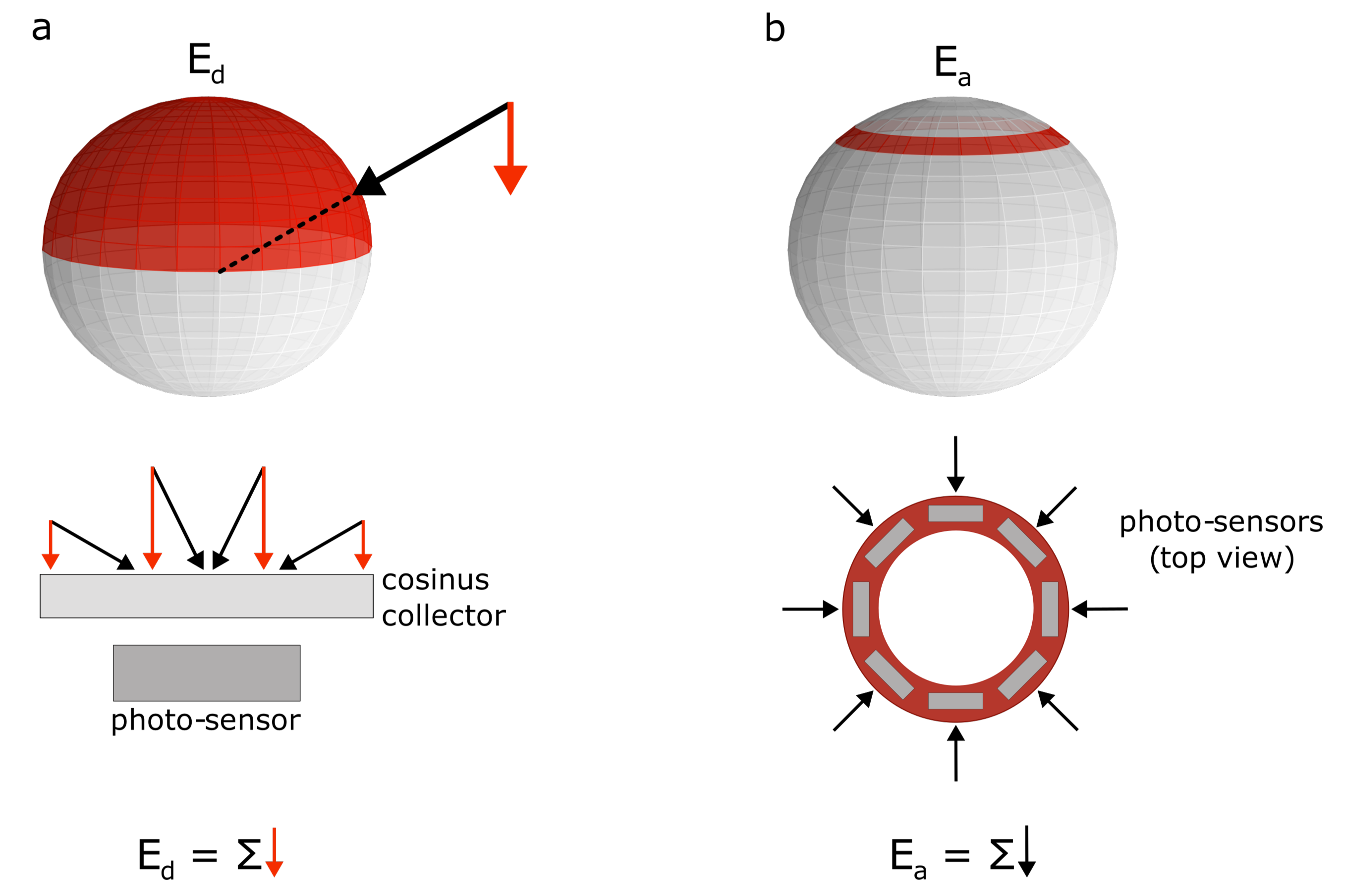
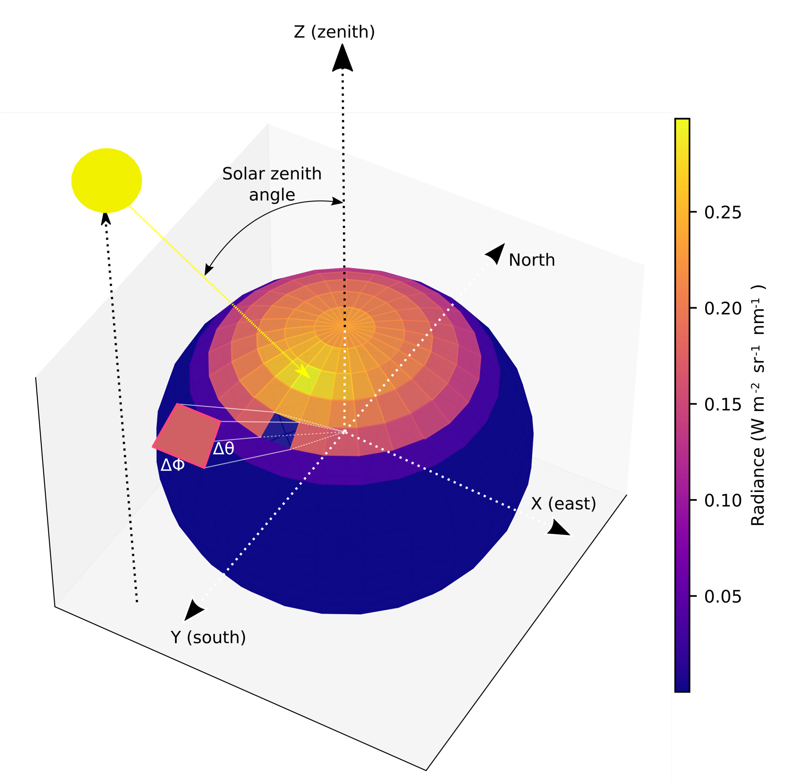
2.1. Theoretical Basis
2.2. Computational Fundamentals: HydoLight as a Numerical Tool
2.3. Definition and Computation of Annular Irradiance and
2.4. Data Sets Description
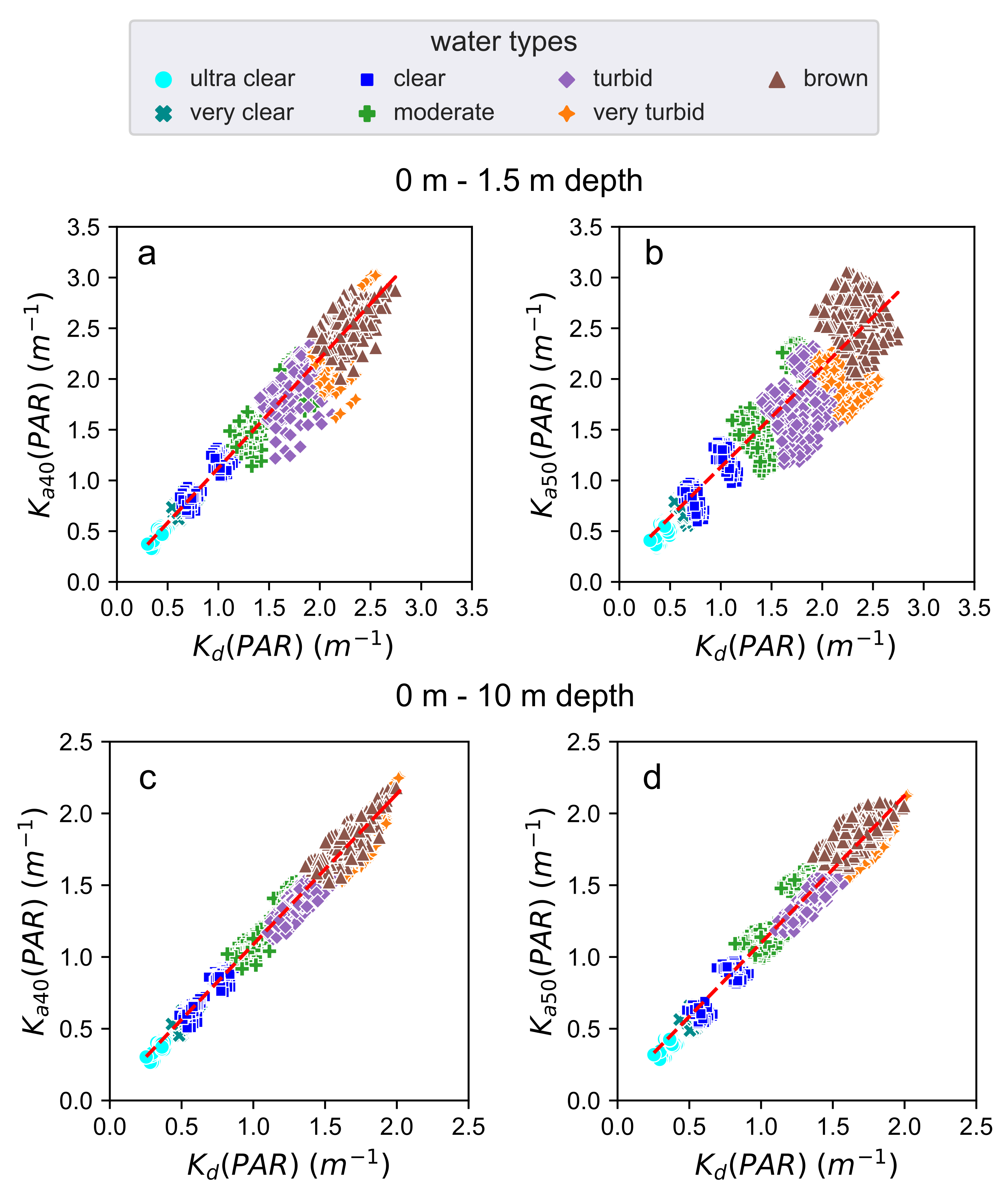
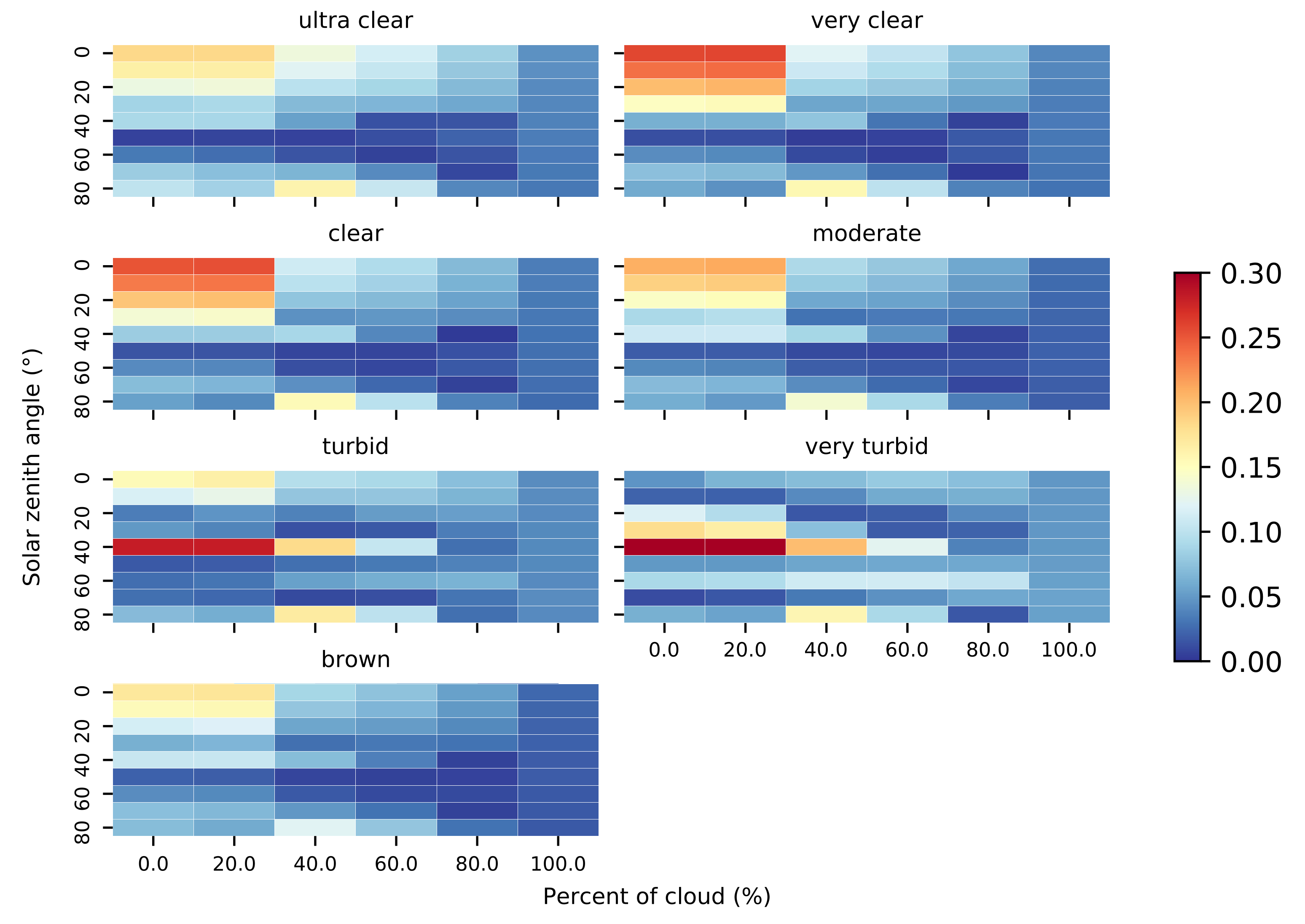
- Water types: we consider in our study from extremely clear to extremely turbid water situations, simulating the kind of waters that could be encountered in estuaries and inland water bodies.
- Wavelengths: We consider wavelengths in between 400 and 700 nm at 5 nm intervals.
- Illumination conditions: we consider a solar zenith angle ranging from to in steps of , and cloud coverage from 0% to 100% in steps of 20%.
- Depth resolution: we follow the depth resolution configurations described in Table 1.
- Data set 1: contains 3024 simulations, following the same parameters described above, with all the different water types (ultra clear, very clear, clear, moderate, turbid, very turbid, brown). Illumination conditions are considered as solar zenith angle range from to at intervals, and cloud coverage from 0% to 100% at 20% intervals. To optimize the number of simulations per water type and lighting conditions, it is considered two different values (maximum and minimum concentrations from Table 2) for each phytoplankton, CDOM, and minerals concentration.
2.5. Methods to Analyze the Relations -, and -
3. Results
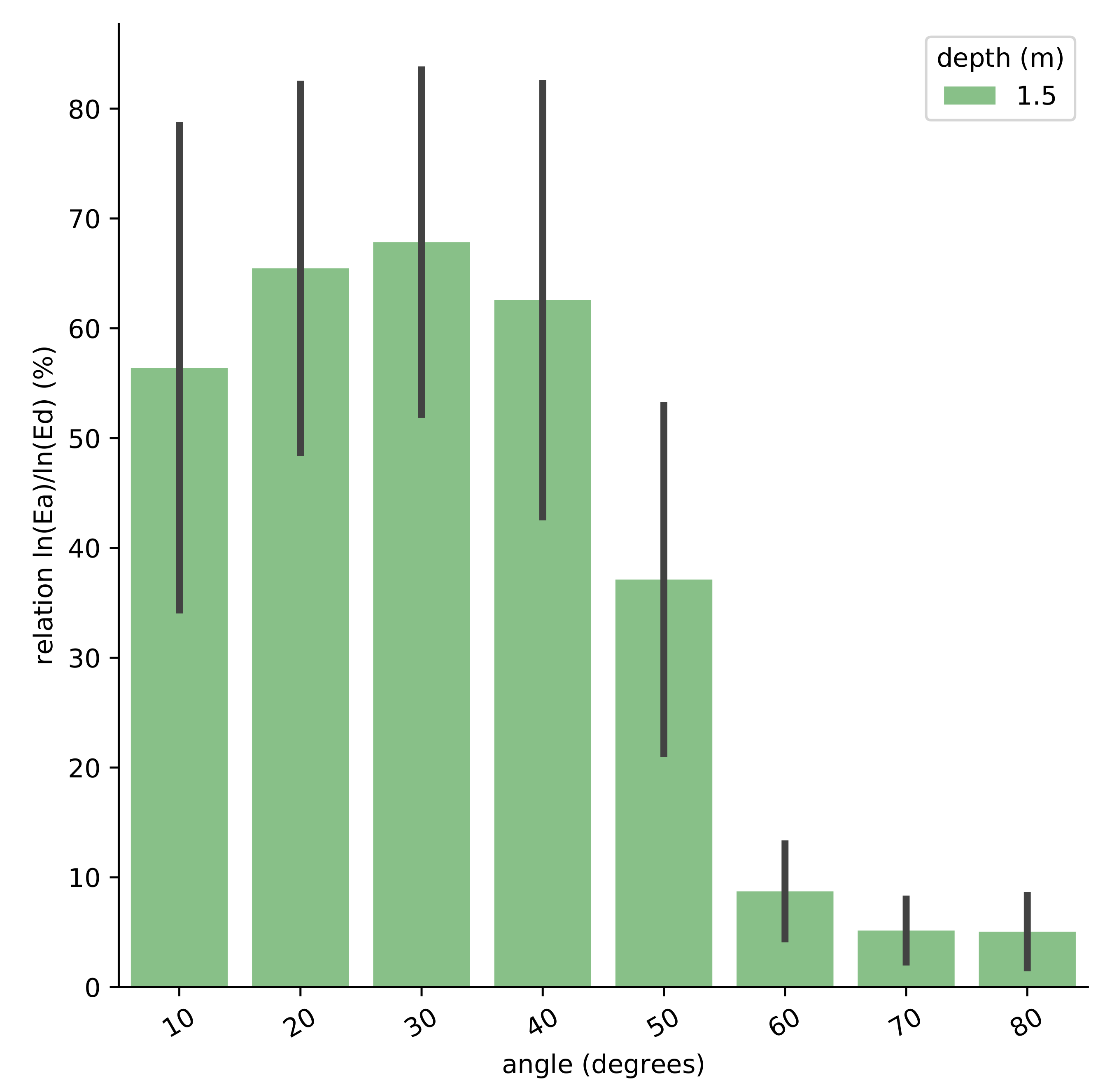
3.1. Optimal Integration Angle
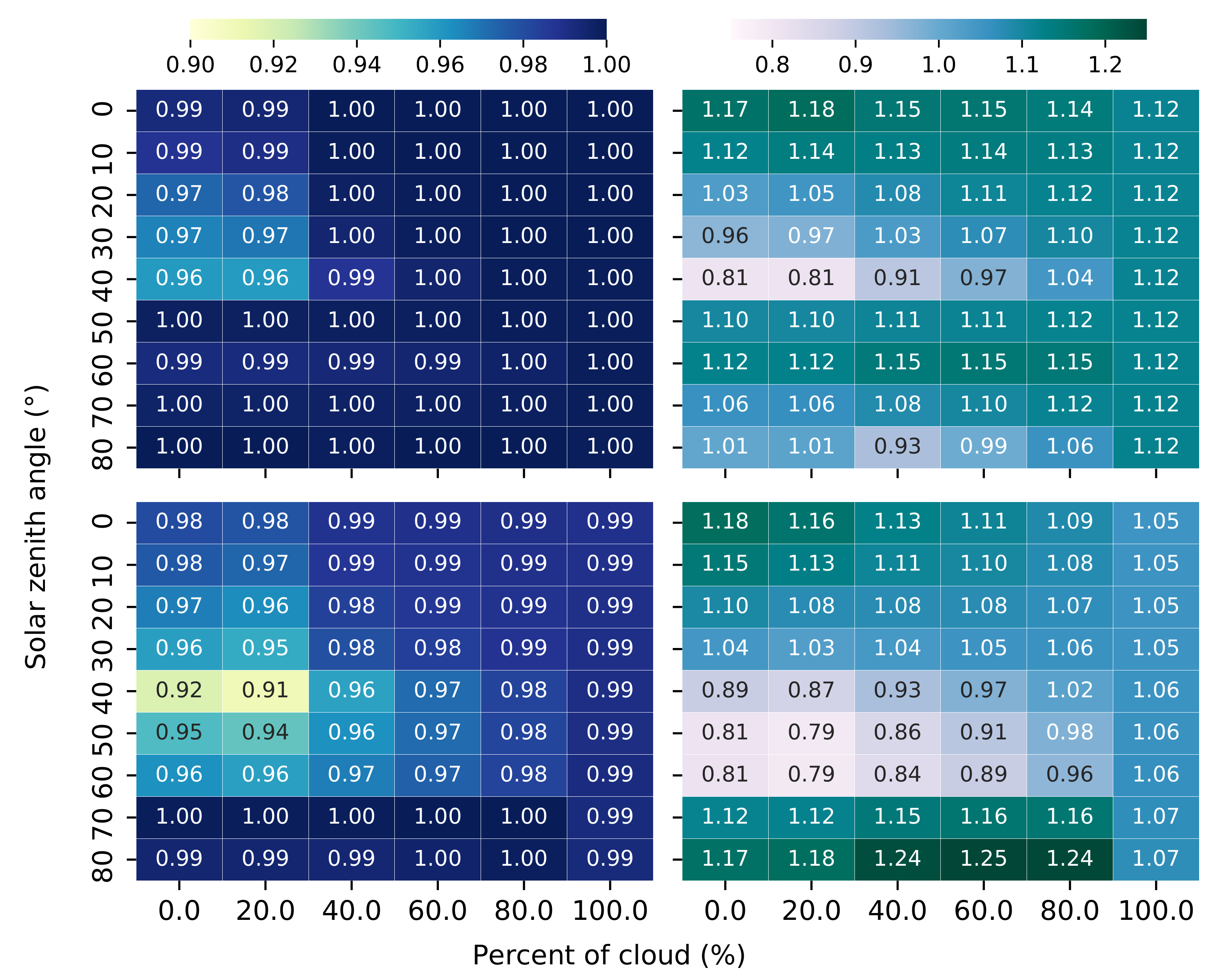
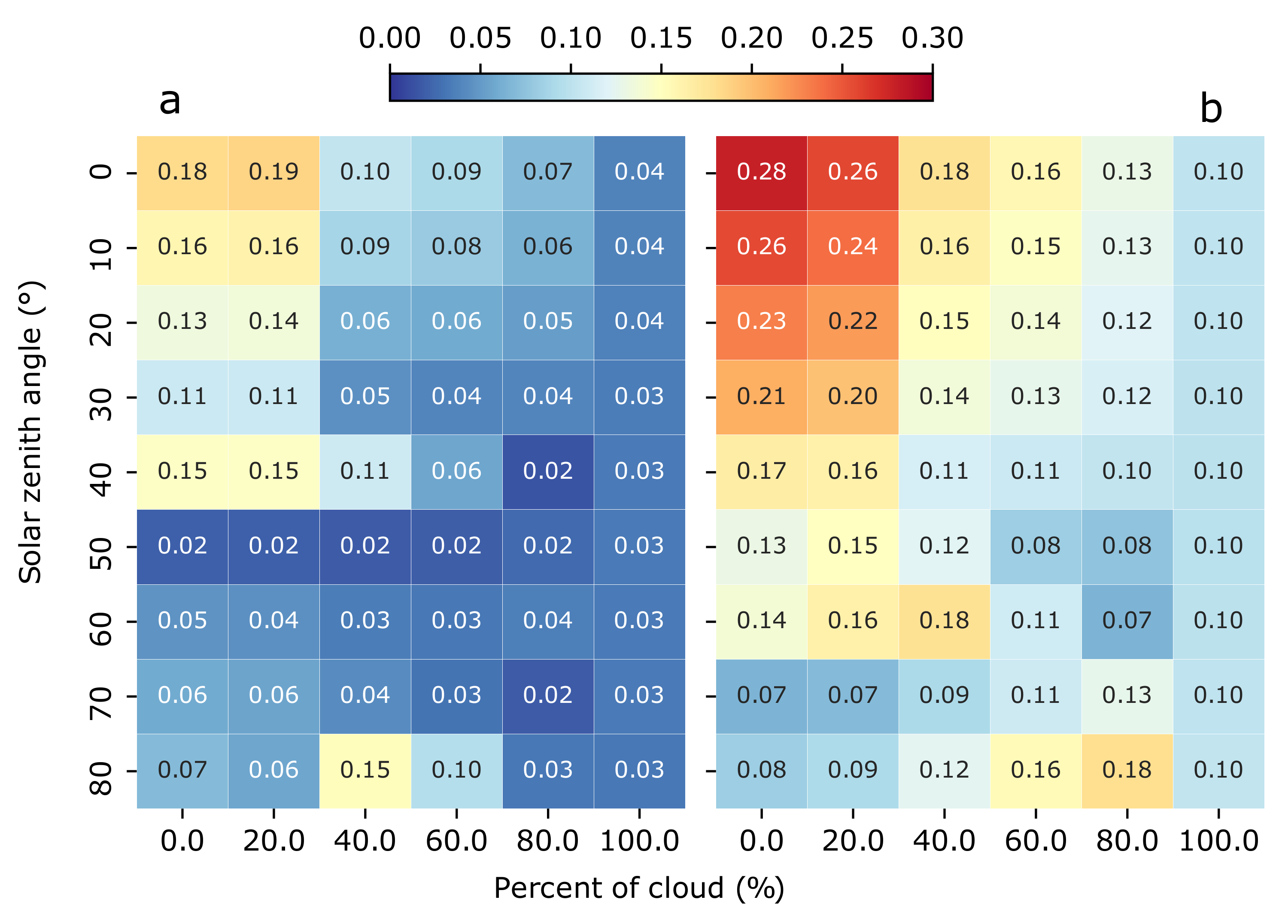
3.2. Comparisons between and
3.3. Comparison between Different Lighting Scenarios
4. Discussion and Conclusions
Author Contributions
Funding
Institutional Review Board Statement
Informed Consent Statement
Data Availability Statement
- The HydroLight configuration files: https://doi.org/10.5281/zenodo.5153536, accessed on 11 August 2021.
- The numerical results: https://doi.org/10.5281/zenodo.5041192, accessed on 11 August 2021.
- The code to generate, process and plot simulations: https://git.csic.es/36579996Z/pysimhydro/-/releases/v1.0.1, accessed on 11 August 2021.
Acknowledgments
Conflicts of Interest
References
- Mobley, C.D.; Chai, F.; Xiu, P.; Sundman, L.K. Impact of improved light calculations on predicted phytoplankton growth and heating in an idealized upwelling-downwelling channel geometry. J. Geophys. Res. Ocean. 2015, 120, 875–892. [Google Scholar] [CrossRef]
- Horion, S.; Bergamino, N.; Stenuite, S.; Descy, J.P.; Plisnier, P.D.; Loiselle, S.A.; Cornet, Y. Optimized extraction of daily bio-optical time series derived from MODIS/Aqua imagery for Lake Tanganyika, Africa. Remote Sens. Environ. 2010, 114, 781–791. [Google Scholar] [CrossRef]
- Cairo, C.T.; Barbosa, C.C.F.; de Moraes Novo, E.M.L.; do Carmo Calijuri, M. Spatial and seasonal variation in diffuse attenuation coefficients of downward irradiance at Ibitinga Reservoir, São Paulo, Brazil. Hydrobiologia 2017, 784, 265–282. [Google Scholar] [CrossRef]
- Mobley, C.D. Light and Water: Radiative Transfer in Natural Waters; Academic Press: Cambridge, MA, USA, 1994. [Google Scholar]
- Sarangi, R.; Chauhan, P.; Nayak, S. Vertical diffuse attenuation coefficient (K d) based optical classification of IRS-P3 MOS-B satellite ocean colour data. J. Earth Syst. Sci. 2002, 111, 237–245. [Google Scholar] [CrossRef]
- Wang, M.; Son, S.; Harding, L.W., Jr. Retrieval of diffuse attenuation coefficient in the Chesapeake Bay and turbid ocean regions for satellite ocean color applications. J. Geophys. Res. Ocean. 2009, 114, C10011. [Google Scholar] [CrossRef]
- Lee, Z.; Carder, K.L.; Arnone, R.A. Deriving inherent optical properties from water color: A multiband quasi-analytical algorithm for optically deep waters. Appl. Opt. 2002, 41, 5755–5772. [Google Scholar] [CrossRef] [PubMed]
- Topp, S.N.; Pavelsky, T.M.; Jensen, D.; Simard, M.; Ross, M.R. Research trends in the use of remote sensing for inland water quality science: Moving towards multidisciplinary applications. Water 2020, 12, 169. [Google Scholar] [CrossRef]
- Tyler, A.N.; Hunter, P.D.; Spyrakos, E.; Groom, S.; Constantinescu, A.M.; Kitchen, J. Developments in Earth observation for the assessment and monitoring of inland, transitional, coastal and shelf-sea waters. Sci. Total Environ. 2016, 572, 1307–1321. [Google Scholar] [CrossRef]
- Kulshreshtha, A.; Shanmugam, P. Estimation of underwater visibility in coastal and inland waters using remote sensing data. Environ. Monit. Assess. 2017, 189, 199. [Google Scholar] [CrossRef]
- Njue, N.; Kroese, J.S.; Gräf, J.; Jacobs, S.; Weeser, B.; Breuer, L.; Rufino, M. Citizen science in hydrological monitoring and ecosystem services management: State of the art and future prospects. Sci. Total Environ. 2019, 693, 133531. [Google Scholar] [CrossRef]
- Vohland, K.; Land-Zandstra, A.; Ceccaroni, L.; Lemmens, R.; Perelló, J.; Ponti, M.; Samson, R.; Wagenknecht, K. The Science of Citizen Science; Springer Nature: Basingstoke, UK, 2021. [Google Scholar]
- Camins, E.; de Haan, W.P.; Salvo, V.S.; Canals, M.; Raffard, A.; Sanchez-Vidal, A. Paddle surfing for science on microplastic pollution. Sci. Total Environ. 2020, 709, 136178. [Google Scholar] [CrossRef]
- Tyler, J.E. The secchi disc. Limnol. Oceanogr. 1968, 13, 1–6. [Google Scholar] [CrossRef]
- Wernand, M.R. On the history of the Secchi disc. J. Eur. Opt. Soc. Rapid Publ. 2010, 5, 10013s. [Google Scholar] [CrossRef]
- Pham, T.N.; Ho, A.P.H.; Nguyen, T.V.; Nguyen, H.M.; Truong, N.H.; Huynh, N.D.; Nguyen, T.H. Development of a Solar-Powered IoT-Based Instrument for Automatic Measurement of Water Clarity. Sensors 2020, 20, 2051. [Google Scholar] [CrossRef]
- Matos, T.; Faria, C.L.; Martins, M.S.; Henriques, R.; Gomes, P.; Goncalves, L.M. Design of a multipoint cost-effective optical instrument for continuous in-situ monitoring of turbidity and sediment. Sensors 2020, 20, 3194. [Google Scholar] [CrossRef]
- Bardaji, R.; Sánchez, A.M.; Simon, C.; Wernand, M.R.; Piera, J. Estimating the underwater diffuse attenuation coefficient with a low-cost instrument: The KdUINO DIY buoy. Sensors 2016, 16, 373. [Google Scholar] [CrossRef] [PubMed]
- Ho, S.Y.F.; Xu, S.J.; Lee, F.W.F. Citizen science: An alternative way for water monitoring in Hong Kong. PLoS ONE 2020, 15, e0238349. [Google Scholar] [CrossRef] [PubMed]
- Mellard, J.P.; Yoshiyama, K.; Litchman, E.; Klausmeier, C.A. The vertical distribution of phytoplankton in stratified water columns. J. Theor. Biol. 2011, 269, 16–30. [Google Scholar] [CrossRef] [PubMed]
- Yoshiyama, K.; Mellard, J.; Litchman, E.; Klausmeier, C. Phytoplankton Competition for Nutrients and Light in a Stratified Water Column. Am. Nat. 2009, 174, 190–203. [Google Scholar] [CrossRef] [PubMed]
- Terzić, E.; Salon, S.; Cossarini, G.; Solidoro, C.; Teruzzi, A.; Miró, A.; Lazzari, P. Impact of interannually variable diffuse attenuation coefficients for downwelling irradiance on biogeochemical modelling. Ocean Model. 2021, 161, 101793. [Google Scholar] [CrossRef]
- Gordon, H.R.; Ding, K. Self-shading of in-water optical instruments. Limnol. Oceanogr. 1992, 37, 491–500. [Google Scholar] [CrossRef]
- Piskozub, J. Effects of surface waves and sea bottom on self-shading of in-water optical instruments. In Ocean Optics XII; International Society for Optics and Photonics: Bellingham, WA, USA, 1994; Volume 2258, pp. 300–308. [Google Scholar]
- Piskozub, J. Influence of instrument casing shape on self-shading of in-water radiation. In Proceedings of the 14th Conference Ocean Optics, Kailua-Kona, HI, USA, November 1998; pp. 10–13. [Google Scholar]
- Aas, E.; Korsbø, B. Self-shading effect by radiance meters on upward radiance observed in coastal waters. Limnol. Oceanogr. 1997, 42, 968–974. [Google Scholar] [CrossRef]
- Piskozub, J.; Weeks, A.R.; Schwarz, J.N.; Robinson, I.S. Self-shading of upwelling irradiance for an instrument with sensors on a sidearm. Appl. Opt. 2000, 39, 1872–1878. [Google Scholar] [CrossRef]
- Leathers, R.A.; Downes, T.V.; Mobley, C.D. Self-shading correction for upwelling sea-surface radiance measurements made with buoyed instruments. Opt. Express 2001, 8, 561–570. [Google Scholar] [CrossRef] [PubMed]
- Piskozub, J. Effect of ship shadow on in-water irradiance measurements. Oceanologia 2004, 46, 103–112. [Google Scholar]
- Silveira, N.; Suresh, T.; Talaulikar, M.; Desa, E.; Prabhu Matondkar, S.; Lotlikar, A. Sources of errors in the measurements of underwater profiling radiometer. Indian J. Mar. Sci. 2014, 43, 88–95. [Google Scholar]
- Mobley, C.D. Radiative transfer in the ocean. Encycl. Ocean. Sci. 2001, 2321–2330. [Google Scholar] [CrossRef]
- Lee, Z.P.; Du, K.P.; Arnone, R. A model for the diffuse attenuation coefficient of downwelling irradiance. J. Geophys. Res. Ocean. 2005, 110, C02016. [Google Scholar] [CrossRef]
- Mobley, C.; Sundman, L. HydroLight 5.2 User’s Guide; Sequoia Scientific: Bellevue, DC, USA, 2013. [Google Scholar]
- Gregg, W.W.; Carder, K.L. A simple spectral solar irradiance model for cloudless maritime atmospheres. Limnol. Oceanogr. 1990, 35, 1657–1675. [Google Scholar] [CrossRef]
- Reinart, A.; Herlevi, A.; Arst, H.; Sipelgas, L. Preliminary optical classification of lakes and coastal waters in Estonia and south Finland. J. Sea Res. 2003, 49, 357–366. [Google Scholar] [CrossRef]
- Lythgoe, J.N. The Ecology of Vision; Oxford Science Publications; Clarendon Press: Wotton-under-Edge, UK, 1979. [Google Scholar]
- Lynch, D.K. Snell’s window in wavy water. Appl. Opt. 2015, 54, B8–B11. [Google Scholar] [CrossRef] [PubMed]
- Darecki, M.; Stramski, D.; Sokólski, M. Measurements of high-frequency light fluctuations induced by sea surface waves with an Underwater Porcupine Radiometer System. J. Geophys. Res. Ocean. 2011, 116, C00H09. [Google Scholar] [CrossRef]
- Stramska, M.; Frye, D. Dependence of apparent optical properties on solar altitude: Experimental results based on mooring data collected in the Sargasso Sea. J. Geophys. Res. Ocean. 1997, 102, 15679–15691. [Google Scholar] [CrossRef]
- Drake, J.M.; Lodge, D.M. Hull fouling is a risk factor for intercontinental species exchange in aquatic ecosystems. Aquat. Invasions 2007, 2, 121–131. [Google Scholar] [CrossRef]
- Garcia-Soto, C.; Seys, J.J.C.; Zielinski, O.; Busch, J.A.; Luna, S.I.; Baez, J.C.; Domegan, C.; Dubsky, K.; Kotynska-Zielinska, I.; Loubat, P.; et al. Marine Citizen Science: Current State in Europe and New Technological Developments. Front. Mar. Sci. 2021, 8, 241. [Google Scholar] [CrossRef]


| Value | Step |
|---|---|
| 2 cm to 50 cm | 2 cm |
| 50 cm to 2 m | 5 cm |
| 2 m to 3 m | 10 cm |
| 3 m to 4 m | 20 cm |
| 4 m to 10 m | 50 cm |
| 10 m to 15 m | 1 m |
| 15 m to 20 m | 5 m |
| chl (mg m) | cdom af(380) | mineral (g m) | ||||
|---|---|---|---|---|---|---|
| Max | Min | Max | Min | Max | Min | |
| ultra clear | 0.0 | 1.0 | 0.0 | 0.6 | 0.0 | 0.8 |
| very clear | 1.0 | 3.0 | 0.5 | 1.5 | 0.5 | 1.5 |
| clear | 2.1 | 7.5 | 1.3 | 3.3 | 1.2 | 2.4 |
| moderate | 3.9 | 17.1 | 5.0 | 12.0 | 1.0 | 6.6 |
| turbid | 19.7 | 41.3 | 5.5 | 9.7 | 10.8 | 18.6 |
| very turbid | 65.2 | 67.6 | 6.1 | 6.7 | 30.3 | 38.7 |
| brown | 3.3 | 20.3 | 18.1 | 22.5 | 2.2 | 7.8 |
| N. Simulations | Water Types | Solar Angle Range | Cloud Coverage | Figure-Table | |
|---|---|---|---|---|---|
| 1 | 2352 | all | Figure 3 and Figure 4, | ||
| 2 | 3024 | all | Figure 5, Figure 6 and Figure 7, Table 4 |
| Depth-Range (m) | ||||||
|---|---|---|---|---|---|---|
| 0–0.2 | 0–0.5 | 0–1.0 | 0–1.5 | 0–5.0 | 0–10.0 | |
| 1.125 | 1.095 | 1.084 | 1.079 | 1.070 | 1.057 | |
| 1.098 | 1.045 | 1.039 | 1.046 | 1.065 | 1.058 | |
| Depth-Range (m) | ||||||
|---|---|---|---|---|---|---|
| 0–0.2 | 0–0.5 | 0–1.0 | 0–1.5 | 0–5.0 | 0–10.0 | |
| 0.083 | 0.075 | 0.070 | 0.068 | 0.061 | 0.056 | |
| 0.140 | 0.154 | 0.149 | 0.138 | 0.112 | 0.095 | |
Publisher’s Note: MDPI stays neutral with regard to jurisdictional claims in published maps and institutional affiliations. |
© 2021 by the authors. Licensee MDPI, Basel, Switzerland. This article is an open access article distributed under the terms and conditions of the Creative Commons Attribution (CC BY) license (https://creativecommons.org/licenses/by/4.0/).
Share and Cite
Rodero, C.; Olmedo, E.; Bardaji, R.; Piera, J. New Radiometric Approaches to Compute Underwater Irradiances: Potential Applications for High-Resolution and Citizen Science-Based Water Quality Monitoring Programs. Sensors 2021, 21, 5537. https://doi.org/10.3390/s21165537
Rodero C, Olmedo E, Bardaji R, Piera J. New Radiometric Approaches to Compute Underwater Irradiances: Potential Applications for High-Resolution and Citizen Science-Based Water Quality Monitoring Programs. Sensors. 2021; 21(16):5537. https://doi.org/10.3390/s21165537
Chicago/Turabian StyleRodero, Carlos, Estrella Olmedo, Raul Bardaji, and Jaume Piera. 2021. "New Radiometric Approaches to Compute Underwater Irradiances: Potential Applications for High-Resolution and Citizen Science-Based Water Quality Monitoring Programs" Sensors 21, no. 16: 5537. https://doi.org/10.3390/s21165537
APA StyleRodero, C., Olmedo, E., Bardaji, R., & Piera, J. (2021). New Radiometric Approaches to Compute Underwater Irradiances: Potential Applications for High-Resolution and Citizen Science-Based Water Quality Monitoring Programs. Sensors, 21(16), 5537. https://doi.org/10.3390/s21165537