
Numerical Investigation of Ferrofluid Preparation during In-Vitro Culture of Cancer Therapy for Magnetic Nanoparticle Hyperthermia


Abstract
:1. Introduction
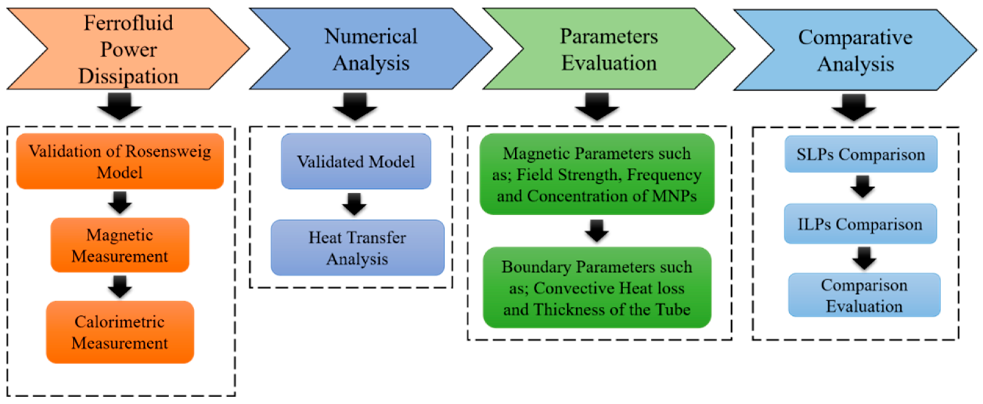
2. Methodology
3. Mathematical Modeling
3.1. Experimental Model
3.2. Magnetic Model
3.3. Calorimetric Model
3.4. Effective Parameters
3.5. Numerical Modeling
- The nanoparticles were homogenously distributed in the MF sample;
- A continuous heat flux was considered from the system to the surroundings;
- The initial temperature of the MF sample was assumed to be 21 °C;
- The convection heat coefficient value was assumed to be 10 W/m2/K;
- The volumetric power generation p (W/m3) was considered as an input parameter to the numerical model and determined using Equation (1).
4. Results and Discussions
4.1. Parameters Obtained from the LRT-Bsed Magnetic Method
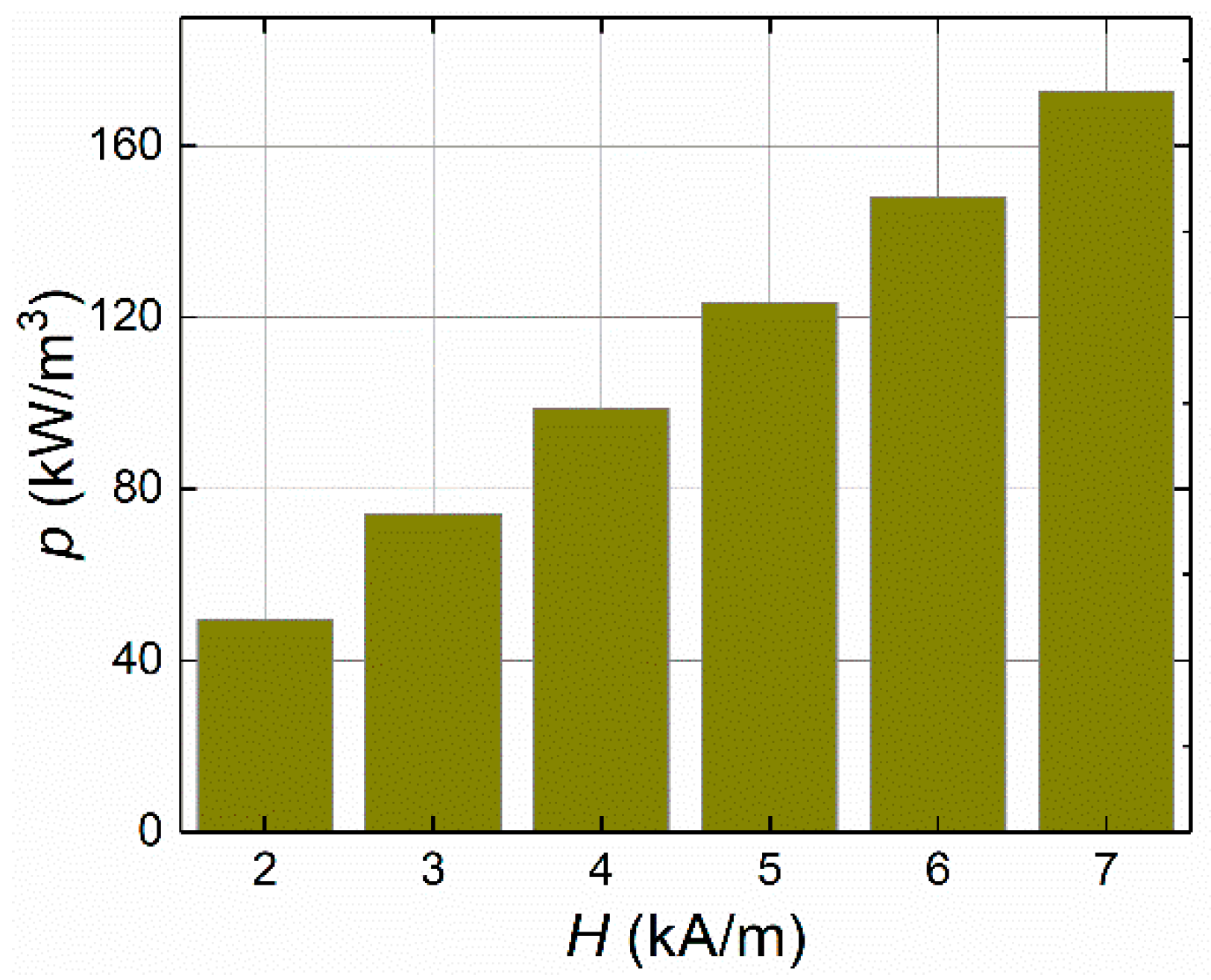
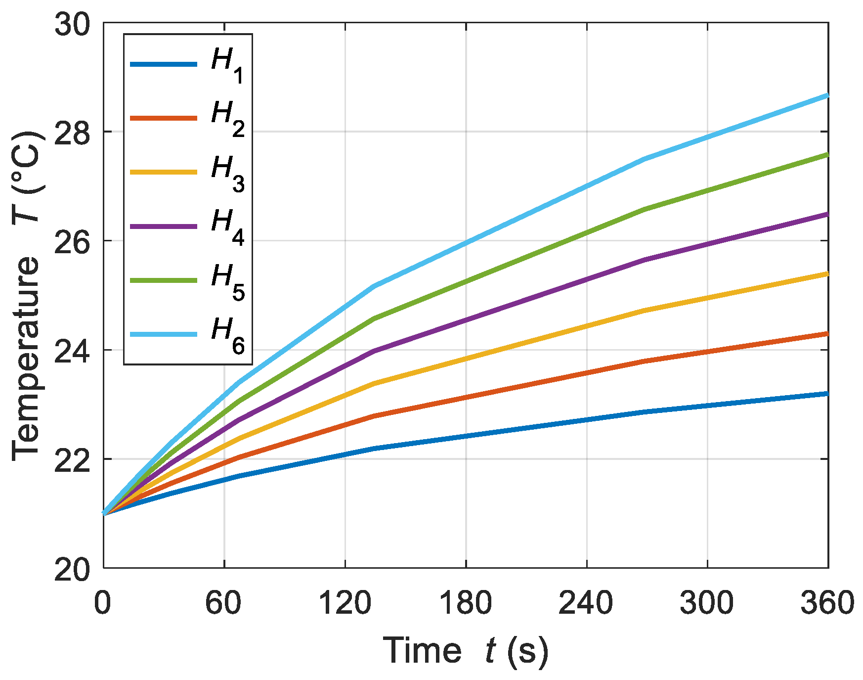
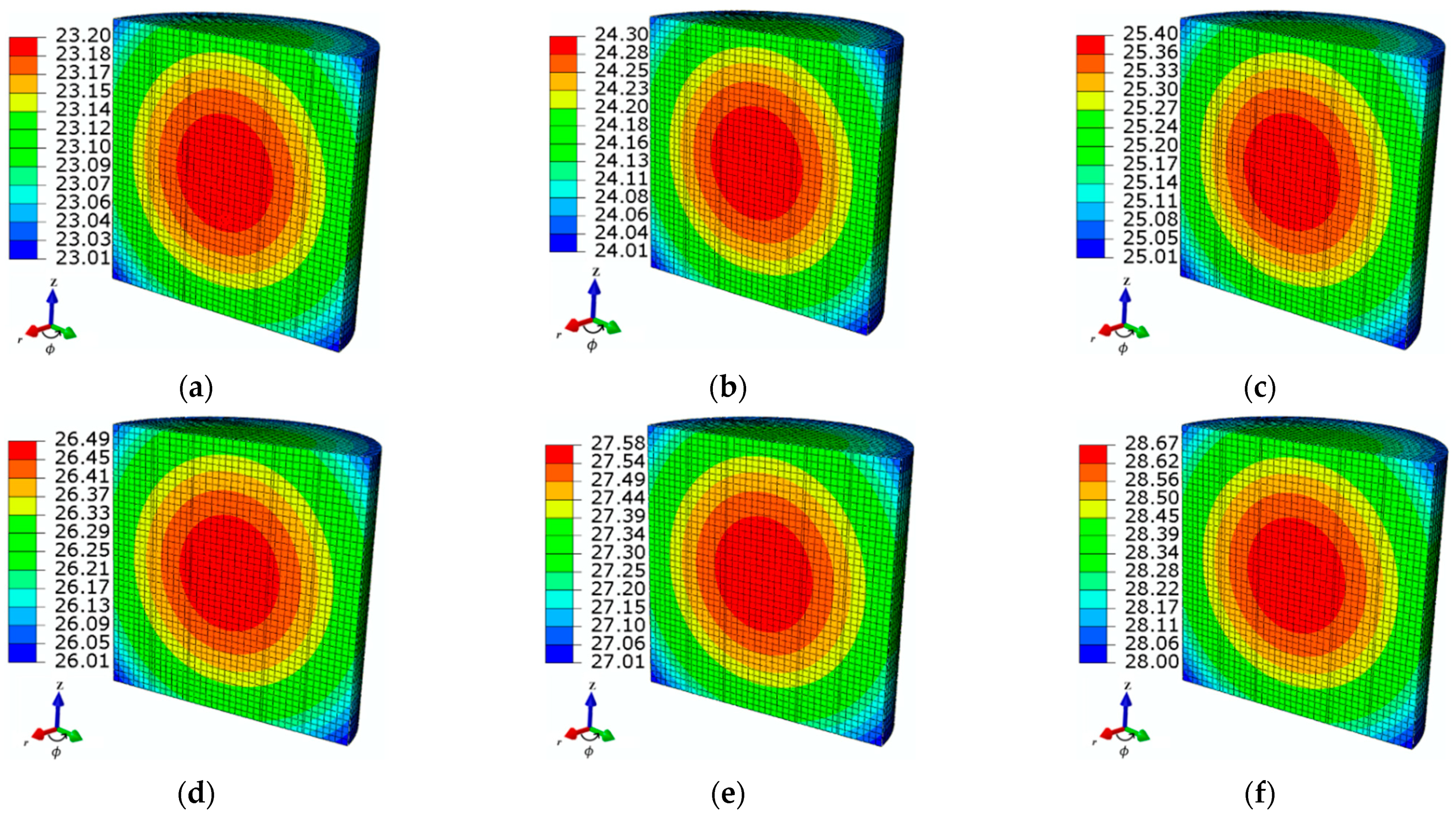
4.1.1. Applied Magnetic Field Strength
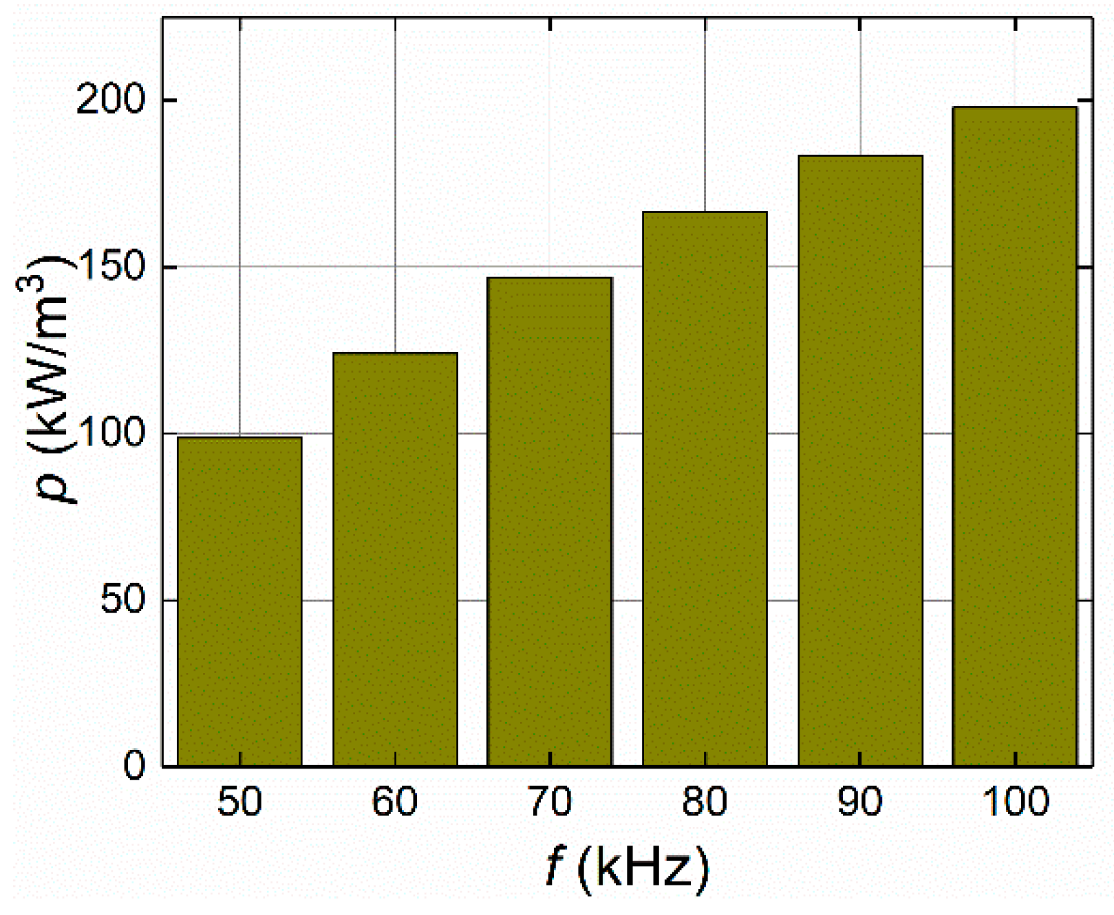
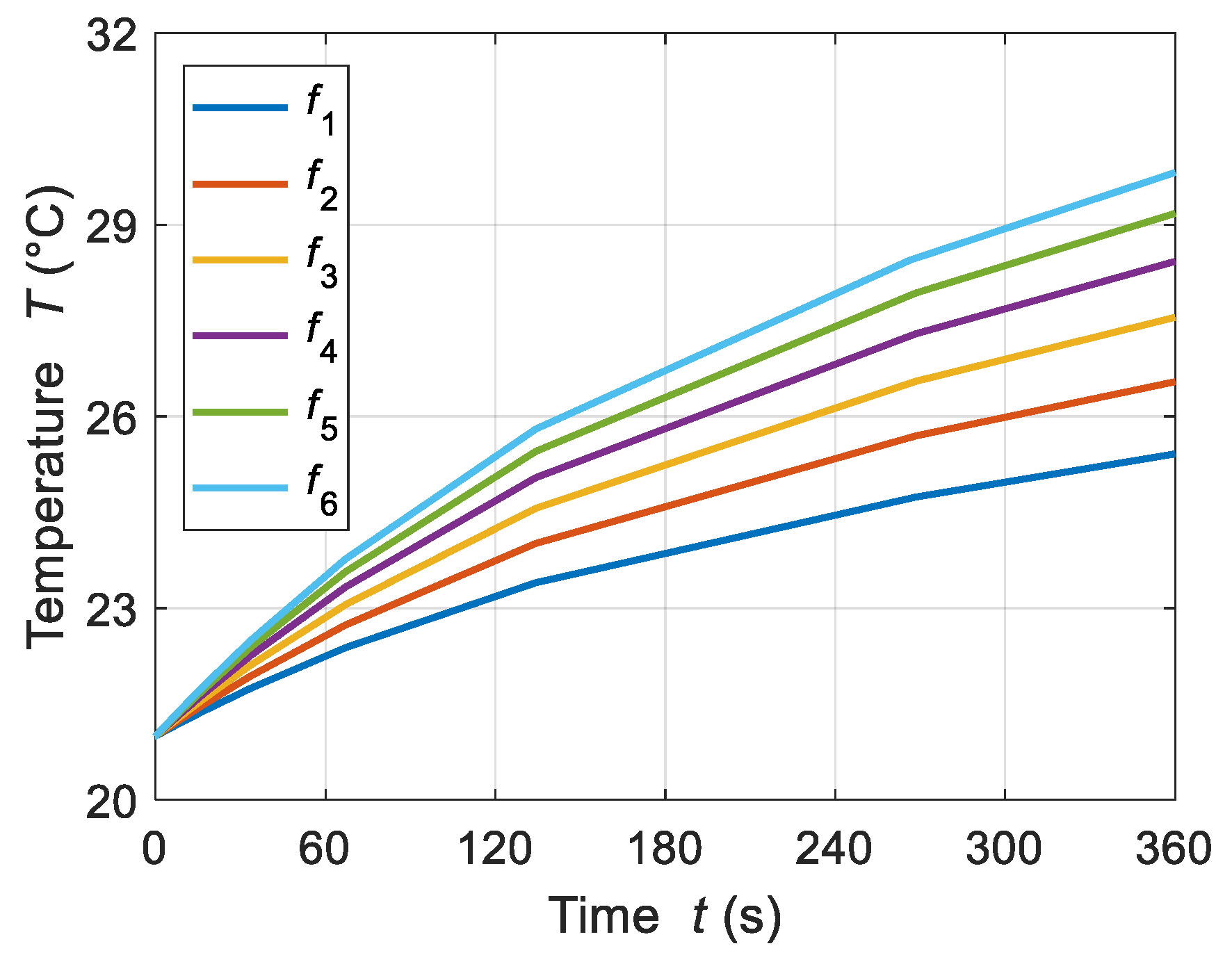
4.1.2. Frequency of the Applied Magnetic Field
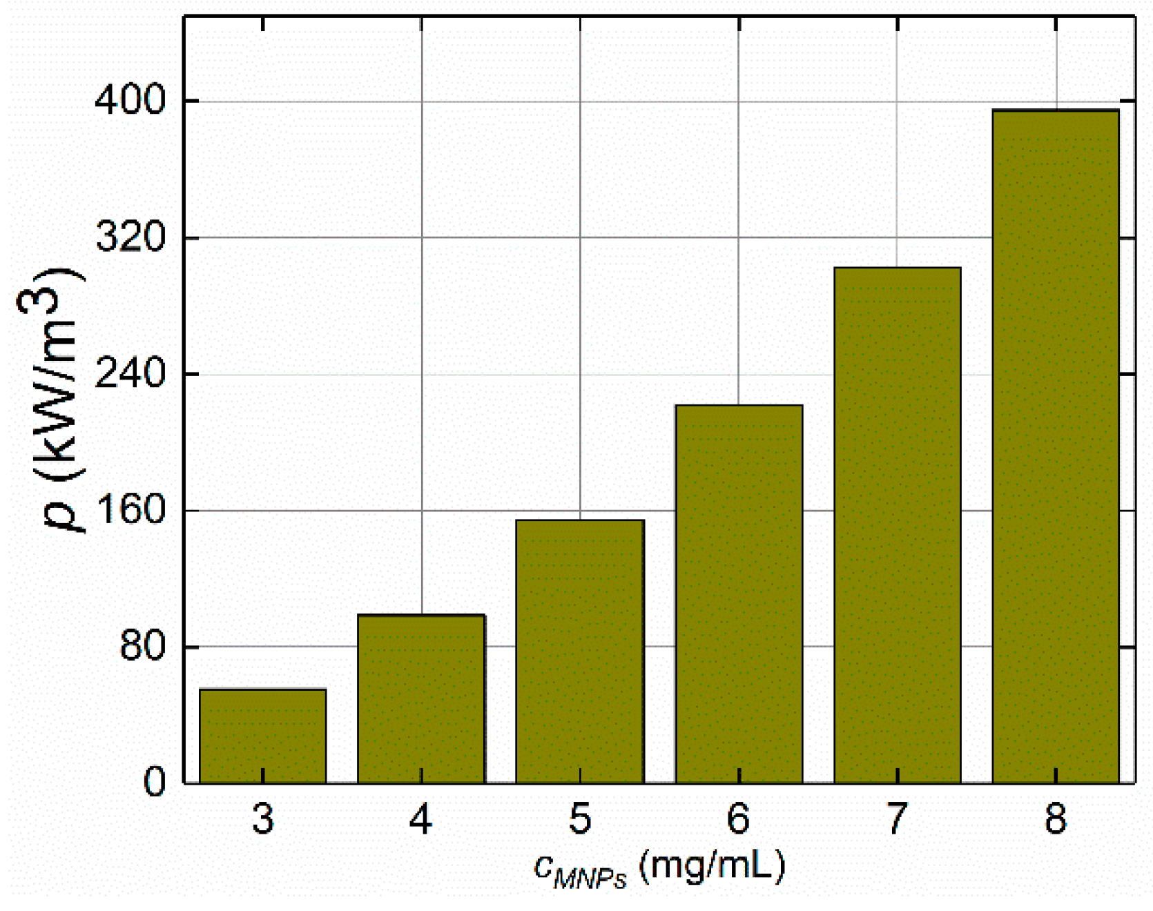
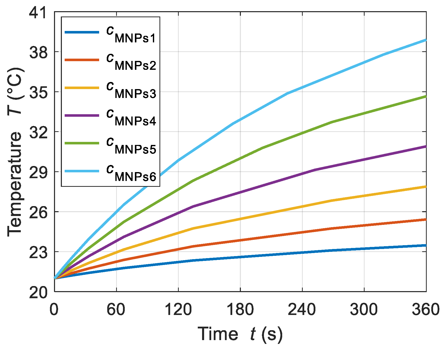
4.1.3. MNP Concentrations
4.2. Boundary Parameters
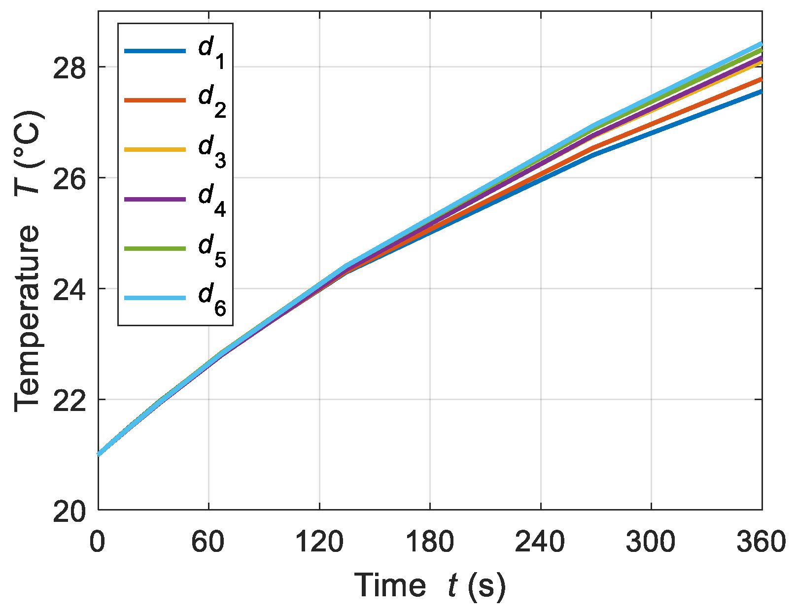
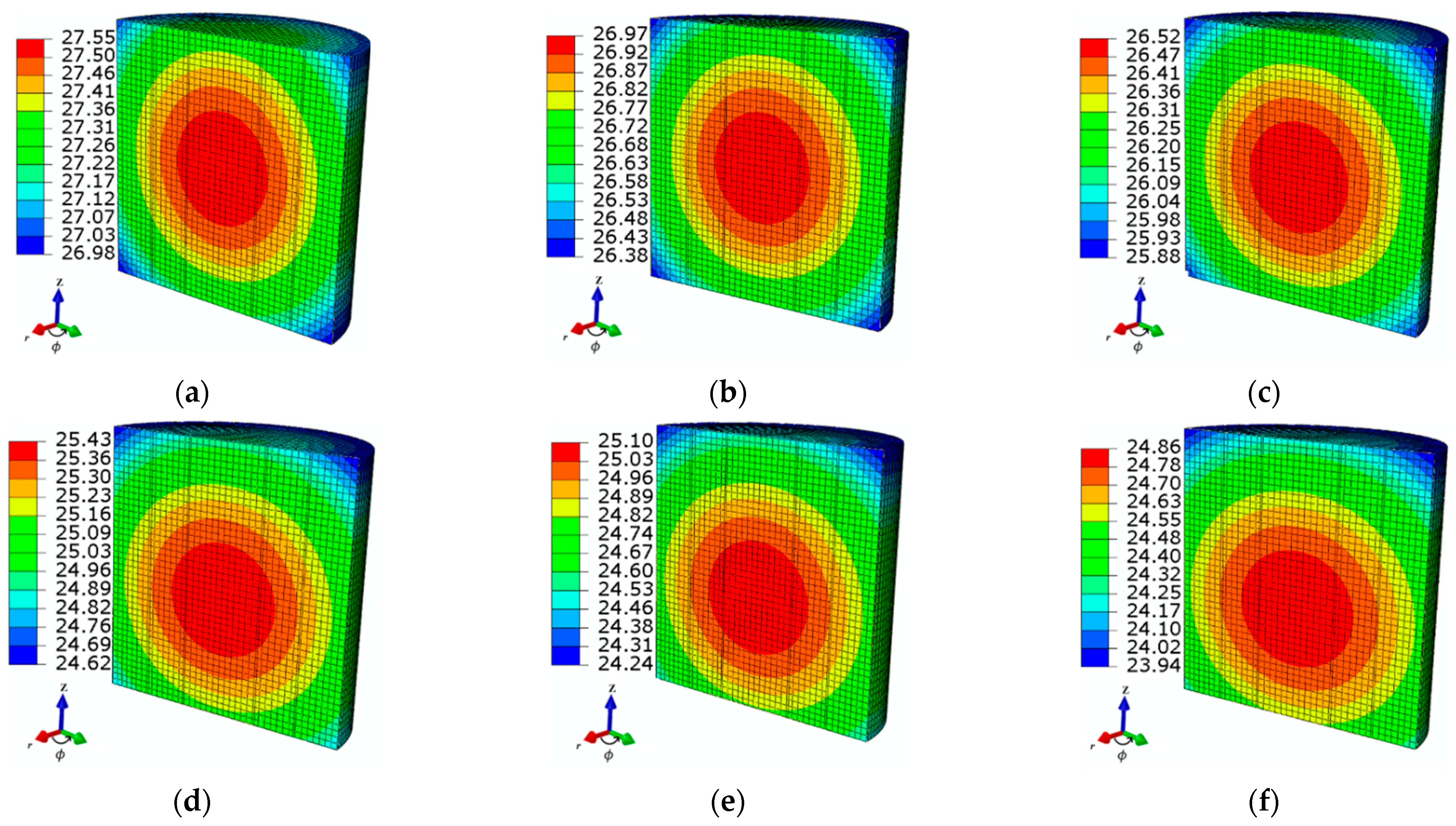
4.2.1. Tube Thickness
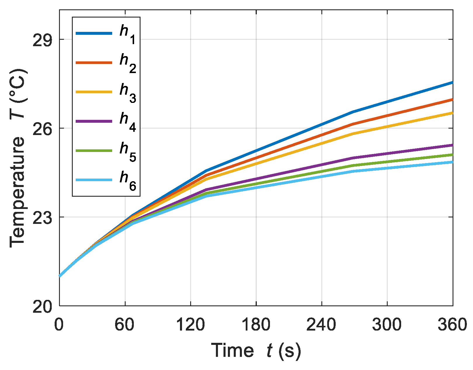
4.2.2. Convective Heat Loss
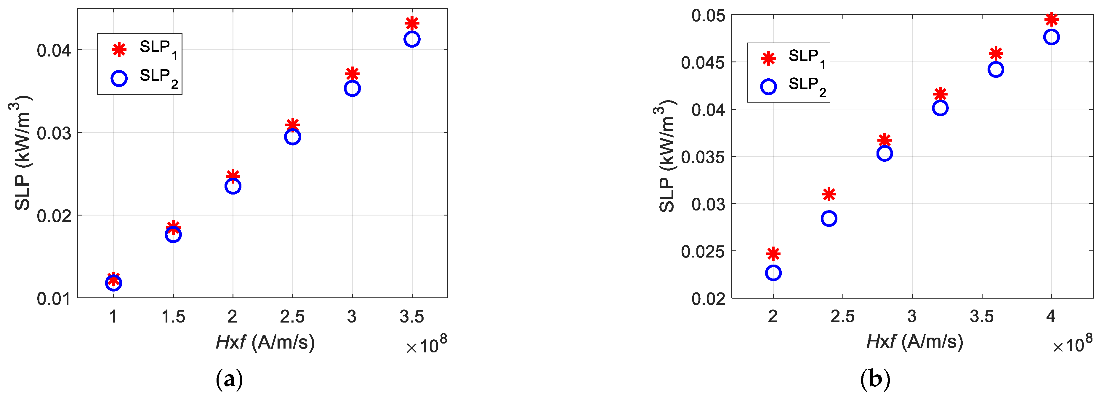
4.3. Comparitive Analysis
5. Conclusions
Supplementary Materials
Author Contributions
Funding
Institutional Review Board Statement
Informed Consent Statement
Data Availability Statement
Conflicts of Interest
Abbreviations
| Abbreviation | Explanation |
| AMF | Applied magnetic field |
| AC | Alternating current |
| EM/EMF | Electromagnetic/electromagnetic field |
| FEA | Finite element analysis |
| FEM | Finite element method |
| ILP | Intrinsic loss power |
| LRT | Linear response theory |
| MF/MFs | Magnetic fluid/magnetic fluids |
| MFH | Magnetic fluid hyperthemria |
| MNP/MNPs | Magnetic nanoparticle/magnetic nanoparticles |
| RE | Relative error |
| SLP | Specific loss power |
References
- Beola, L.; Grazú, V.; Fernández-Afonso, Y.; Fratila, R.M.; de las Heras, M.; de la Fuente, J.M.; Gutiérrez, L.; Asín, L. Critical parameters to improve pancreatic cancer treatment using magnetic hyperthermia: Field conditions, immune response, and particle biodistribution. ACS Appl. Mater. Interfaces 2021, 13, 12982–12996. [Google Scholar] [CrossRef]
- Farzin, A.; Etesami, S.A.; Quint, J.; Memic, A.; Tamayol, A. Magnetic nanoparticles in cancer therapy and diagnosis. Adv. Healthcare Mater. 2020, 9, 1901058. [Google Scholar] [CrossRef] [PubMed]
- Jia, D.; Liu, J. Evaluation on the capacity of selectively heating vessel-rich-skin to realize noninvasive whole body hyperthermia. Int. J. Therm. Sci. 2010, 49, 1968–1976. [Google Scholar] [CrossRef]
- Tang, Y.; Jin, T.; Flesch, R.C. Impact of different infusion rates on mass diffusion and treatment temperature field during magnetic hyperthermia. Int. J. Heat Mass Transf. 2018, 124, 639–645. [Google Scholar] [CrossRef]
- Miaskowski, A.; Subramanian, M. Numerical model for magnetic fluid hyperthermia in a realistic breast phantom: Calorimetric calibration and treatment planning. Int. J. Mol. Sci. 2019, 20, 4644. [Google Scholar] [CrossRef] [PubMed] [Green Version]
- Yuan, P.; Yang, C.-S.; Liu, S.-F. Temperature analysis of a biological tissue during hyperthermia therapy in the thermal non-equilibrium porous model. Int. J. Mol. Sci. 2014, 78, 124–131. [Google Scholar] [CrossRef]
- Raouf, I.; Khalid, S.; Khan, A.; Lee, J.; Kim, H.S.; Kim, M.-H. A review on numerical modeling for magnetic nanoparticle hyperthermia: Progress and challenges. J. Therm. Biol. 2020, 91, 102644. [Google Scholar] [CrossRef]
- Soetaert, F.; Korangath, P.; Serantes, D.; Fiering, S.; Ivkov, R. Cancer therapy with iron oxide nanoparticles: Agents of thermal and immune therapies. Adv. Drug Deliv. Rev. 2020, 163–164, 65–83. [Google Scholar] [CrossRef]
- Yu, B.; Jiang, X. Temperature prediction by a fractional heat conduction model for the bi-layered spherical tissue in the hyperthermia experiment. Int. J. Therm. Sci. 2019, 145, 105990. [Google Scholar] [CrossRef]
- Dutta, J.; Kundu, B.; Yook, S.-J. Three-dimensional thermal assessment in cancerous tumors based on local thermal non-equilibrium approach for hyperthermia treatment. Int. J. Therm. Sci. 2021, 159, 106591. [Google Scholar] [CrossRef]
- Tang, Y.; Jin, T.; Flesch, R.C.C.; Gao, Y.; He, M. Effect of nanofluid distribution on therapeutic effect considering transient bio-tissue temperature during magnetic hyperthermia. J. Magn. Magn. Mater. 2021, 517, 167391. [Google Scholar] [CrossRef]
- Gas, P.; Miaskowski, A.; Subramanian, M. In silico study on tumor-size-dependent thermal profiles inside an anthropomorphic female breast phantom subjected to multi-dipole antenna array. Int. J. Mol. Sci. 2020, 21, 8597. [Google Scholar] [CrossRef]
- Reis, R.F.; dos Santos Loureiro, F.; Lobosco, M. 3D numerical simulations on GPUs of hyperthermia with nanoparticles by a nonlinear bioheat model. J. Comput. Appl. Math. 2016, 295, 35–47. [Google Scholar] [CrossRef]
- Raouf, I.; Lee, J.; Kim, H.S.; Kim, M.-H. Parametric investigations of magnetic nanoparticles hyperthermia in ferrofluid using finite element analysis. Int. J. Therm. Sci. 2021, 159, 106604. [Google Scholar] [CrossRef]
- Paruch, M. Identification of the degree of tumor destruction on the basis of the arrhenius integral using the evolutionary algorithm. Int. J. Therm. Sci. 2018, 130, 507–517. [Google Scholar] [CrossRef]
- Roohi, R.; Heydari, M.H.; Avazzadeh, Z. Optimal control of hyperthermia thermal damage based on tumor configuration. Results Phys. 2021, 23, 103992. [Google Scholar] [CrossRef]
- Çitoğlu, S.; Coşkun, Ö.D.; Tung, L.D.; Onur, M.A.; Kim Thanh, N.T. DMSA-coated cubic iron oxide nanoparticles as potential therapeutic agents. Nanomedicine 2021, 16, 925–941. [Google Scholar] [CrossRef] [PubMed]
- Archilla, D.; López-Sánchez, J.; Hernando, A.; Navarro, E.; Marín, P. Boosting the tunable microwave scattering signature of sensing array platforms consisting of amorphous ferromagnetic Fe2.25Co72.75Si10B15 microwires and its amplification by intercalating Cu microwires. Nanomaterials 2021, 11, 920. [Google Scholar] [CrossRef]
- Dippong, T.; Levei, E.A.; Cadar, O. Recent advances in synthesis and applications of MFe2O4 (M = Co, Cu, Mn, Ni, Zn) nanoparticles. Nanomaterials 2021, 11, 1560. [Google Scholar] [CrossRef]
- Crăciunescu, I.; Palade, P.; Iacob, N.; Ispas, G.M.; Stanciu, A.E.; Kuncser, V.; Turcu, R.P. High-performance functionalized magnetic nanoparticles with tailored sizes and shapes for localized hyperthermia applications. J. Phys. Chem. C 2021, 125, 11132–11146. [Google Scholar] [CrossRef]
- Sheikhpour, M.; Arabi, M.; Kasaeian, A.; Rokn Rabei, A.; Taherian, Z. Role of nanofluids in drug delivery and biomedical technology. Nanotechnol. Sci. Appl. 2020, 13, 47–59. [Google Scholar] [CrossRef]
- Albinali, K.; Zagho, M.; Deng, Y.; Elzatahry, A. A Perspective on magnetic core–shell carriers for responsive and targeted drug delivery systems. Int. J. Nanomed. 2019, 14, 1707–1723. [Google Scholar] [CrossRef] [Green Version]
- Amin, M.; Huang, W.; Seynhaeve, A.L.B.; Ten Hagen, T.L.M. Hyperthermia and temperature-sensitive nanomaterials for spatiotemporal drug delivery to solid tumors. Pharmaceutics 2020, 12, 1007. [Google Scholar] [CrossRef]
- Moloudi, K.; Samadian, H.; Jaymand, M.; Khodamoradi, E.; Hoseini-Ghahfarokhi, M.; Fathi, F. Iron oxide/gold nanoparticles-decorated reduced graphene oxide nanohybrid as the thermo-radiotherapy agent. IET Nanobiotechnol. 2020, 14, 428–432. [Google Scholar] [CrossRef]
- Taufiq, A.; Wahyuni, N.; Saputro, R.E.; Mufti, N.; Hidayat, A.; Yuliantika, D.; Hidayat, N. Investigation of structural, magnetic and antibacterial activities of CrxFe3-xO4 ferrofluids. Mol. Cryst. Liq. 2019, 694, 60–72. [Google Scholar] [CrossRef]
- Lee, J.-H.; Kim, B.; Kim, Y.; Kim, S.-K. Ultra-high rate of temperature increment from superparamagnetic nanoparticles for highly efficient hyperthermia. Sci. Rep. 2021, 11, 4969. [Google Scholar] [CrossRef]
- Anilkumar, T.S.; Lu, Y.-J.; Chen, J.-P. Optimization of the preparation of magnetic liposomes for the combined use of magnetic hyperthermia and photothermia in dual magneto-photothermal cancer therapy. Int. J. Mol. Sci. 2020, 21, 5187. [Google Scholar] [CrossRef]
- Yin, Y.; Ren, Y.; Li, H.; Qi, H. Characteristic analysis of light and heat transfer in photothermal therapy using multiple-light-source heating strategy. Int. J. Therm. Sci. 2020, 158, 1–9. [Google Scholar] [CrossRef]
- Bienia, A.; Wiecheć-Cudak, O.; Murzyn, A.A.; Krzykawska-Serda, M. Photodynamic therapy and hyperthermia in combination treatment—Neglected forces in the fight against cancer. Pharmaceutics 2021, 13, 1147. [Google Scholar] [CrossRef]
- Szczech, M. Experimental studies of magnetic fluid seals and their influence on rolling bearings. J. Magn. 2020, 25, 48–55. [Google Scholar] [CrossRef]
- Kozissnik, B.; Bohorquez, A.C.; Dobson, J.; Rinaldi, C. Magnetic fluid hyperthermia: Advances, challenges, and opportunity. Int. J. Hyperth. 2013, 29, 706–714. [Google Scholar] [CrossRef] [PubMed]
- Herea, D.-D.; Danceanu, C.; Radu, E.; Labusca, L.; Lupu, N.; Chiriac, H. Comparative effects of magnetic and water-based hyperthermia treatments on human osteosarcoma cells. Int. J. Nanomed. 2018, 13, 5743–5751. [Google Scholar] [CrossRef] [PubMed] [Green Version]
- Al Faruque, H.; Choi, E.-S.; Lee, H.-R.; Kim, J.-H.; Park, S.; Kim, E. Targeted removal of leukemia cells from the circulating system by whole-body magnetic hyperthermia in mice. Nanoscale 2020, 12, 2773–2786. [Google Scholar] [CrossRef] [PubMed]
- Jamil, M.; Ng, E.Y.K. To optimize the efficacy of bioheat transfer in capacitive hyperthermia: A physical perspective. J. Therm. Biol. 2013, 38, 272–279. [Google Scholar] [CrossRef]
- Hedayatnasab, Z.; Dabbagh, A.; Abnisa, F.; Wan Daud, W.M.A. Polycaprolactone-coated superparamagnetic iron oxide nanoparticles for in vitro magnetic hyperthermia therapy of cancer. Eur. Polym. J. 2020, 133, 109789. [Google Scholar] [CrossRef]
- Iglesias, G.R.; Jabalera, Y.; Peigneux, A.; Checa Fernández, B.L.; Delgado, Á.V.; Jimenez-Lopez, C. Enhancement of magnetic hyperthermia by mixing synthetic inorganic and biomimetic magnetic nanoparticles. Pharmaceutics 2019, 11, 273. [Google Scholar] [CrossRef] [Green Version]
- Iacovita, C.; Fizeșan, I.; Pop, A.; Scorus, L.; Dudric, R.; Stiufiuc, G.; Vedeanu, N.; Tetean, R.; Loghin, F.; Stiufiuc, R.; et al. In vitro intracellular hyperthermia of iron oxide magnetic nanoparticles, synthesized at high temperature by a polyol process. Pharmaceutics 2020, 12, 424. [Google Scholar] [CrossRef]
- Nauman, M.; Alnasir, M.H.; Hamayun, M.A.; Wang, Y.; Shatruk, M.; Manzoor, S. Size-dependent magnetic and magnetothermal properties of gadolinium silicide nanoparticles. RSC Adv. 2020, 10, 28383–28389. [Google Scholar] [CrossRef]
- Shi, D.; Sadat, M.E.; Dunn, A.W.; Mast, D.B. Photo-fluorescent and magnetic properties of iron oxide nanoparticles for biomedical applications. Nanoscale 2015, 7, 8209–8232. [Google Scholar] [CrossRef]
- Fuentes-García, J.A.; Carvalho Alavarse, A.; Moreno Maldonado, A.C.; Toro-Córdova, A.; Ibarra, M.R.; Goya, G.F. Simple sonochemical method to optimize the heating efficiency of magnetic nanoparticles for magnetic fluid hyperthermia. ACS Omega 2020, 5, 26357–26364. [Google Scholar] [CrossRef]
- Zhang, X.; Zhang, Y. Experimental study on enhanced heat transfer and flow performance of magnetic nanofluids under alternating magnetic field. Int. J. Therm. Sci. 2021, 164, 106897. [Google Scholar] [CrossRef]
- Dutz, S.; Hergt, R. Magnetic nanoparticle heating and heat transfer on a microscale: Basic principles, realities and physical limitations of hyperthermia for tumour therapy. Int. J. Hyperth. 2013, 29, 790–800. [Google Scholar] [CrossRef]
- Gas, P.; Miaskowski, A. Specifying the ferrofluid parameters important from the viewpoint of magnetic fluid hyperthermia. In Proceedings of the 2015 Selected Problems of Electrical Engineering and Electronics (WZEE), Kielce, Poland, 17–19 September 2015; pp. 1–6. [Google Scholar] [CrossRef]
- Da Silva, F.A.S.; de Campos, M.F. Study of heating curves generated by magnetite nanoparticles aiming application in magnetic hyperthermia. Braz. J. Chem. Eng. 2020, 37, 543–553. [Google Scholar] [CrossRef]
- Beković, M.; Trbušić, M.; Gyergyek, S.; Trlep, M.; Jesenik, M.; Szabo, P.; Hamler, A. Numerical model for determining the magnetic loss of magnetic fluids. Materials 2019, 12, 591. [Google Scholar] [CrossRef] [Green Version]
- Rosensweig, R.E. Heating magnetic fluid with alternating magnetic field. J. Magn. Magn. Mater. 2002, 252, 370–374. [Google Scholar] [CrossRef]
- Soetaert, F.; Kandala, S.K.; Bakuzis, A.; Ivkov, R. Experimental estimation and analysis of variance of the measured loss power of magnetic nanoparticles. Sci. Rep. 2017, 7, 6661. [Google Scholar] [CrossRef] [PubMed] [Green Version]
- Wildeboer, R.R.; Southern, P.; Pankhurst, Q.A. On the reliable measurement of specific absorption rates and intrinsic loss parameters in magnetic hyperthermia materials. J. Phys. D Appl. Phys. 2014, 47, 495003. [Google Scholar] [CrossRef]
- Alberti, M.; Prina-Mello, A. Smart model of intrinsic loss power of SPIONs in hyperthermia treatment. J. Magn. Magn. Mater. 2020, 502, 166493. [Google Scholar] [CrossRef]
- Sabale, S.; Jadhav, V.; Mane-Gavade, S.; Yu, X.-Y. Superparamagnetic CoFe2O4@Au with high specific absorption rate and intrinsic loss power for magnetic fluid hyperthermia applications. Acta Metall. Sin. 2019, 32, 719–725. [Google Scholar] [CrossRef] [Green Version]
- Piehler, S.; Dähring, H.; Grandke, J.; Göring, J.; Couleaud, P.; Aires, A.; Cortajarena, A.L.; Courty, J.; Latorre, A.; Somoza, Á.; et al. Iron oxide nanoparticles as carriers for DOX and magnetic hyperthermia after intratumoral application into breast cancer in mice: Impact and future perspectives. Nanomaterials 2020, 10, 1016. [Google Scholar] [CrossRef]
- Lanier, O.L.; Korotych, O.I.; Monsalve, A.G.; Wable, D.; Savliwala, S.; Grooms, N.W.F.; Nacea, C.; Tuitt, O.R.; Dobson, J. Evaluation of magnetic nanoparticles for magnetic fluid hyperthermia. Int. J. Hyperth. 2019, 36, 686–700. [Google Scholar] [CrossRef] [PubMed]
- Castellanos-Rubio, I.; Rodrigo, I.; Olazagoitia-Garmendia, A.; Arriortua, O.; de Muro, I.G.; Garitaonandia, J.S.; Bilbao, J.R.; Fdez-Gubieda, M.L.; Plazaola, F.; Orue, I.; et al. Highly reproducible hyperthermia response in water, agar, and cellular environment by discretely PEGylated magnetite nanoparticles. ACS Appl. Mater. 2020, 12, 27917–27929. [Google Scholar] [CrossRef] [PubMed]
- Osaci, M.; Cacciola, M. About the influence of the colloidal magnetic nanoparticles coating on the specific loss power in magnetic hyperthermia. J. Magn. Magn. Mater. 2021, 519, 167451. [Google Scholar] [CrossRef]
- Gas, P.; Kurgan, E. Cooling effects inside water-cooled inductors for magnetic fluid hyperthermia. In Proceedings of the 2017 Progress in Applied Electrical Engineering (PAEE), Koscielisko, Poland, 25–30 June 2017; pp. 1–4. [Google Scholar] [CrossRef]
- Gas, P. Behavior of helical coil with water cooling channel and temperature dependent conductivity of copper winding used for MFH purpose. IOP Conf. Ser. Environ. Earth Sci. 2019, 214, 012124. [Google Scholar] [CrossRef]
- Hadadian, Y.; Azimbagirad, M.; Navas, E.A.; Pavan, T.Z. A versatile induction heating system for magnetic hyperthermia studies under different experimental conditions. Rev. Sci. Instrum. 2019, 90, 074701. [Google Scholar] [CrossRef] [PubMed]
- Huang, S.; Wang, S.Y.; Gupta, A.; Borca-Tasciuc, D.A.; Salon, S.J. On the measurement technique for specific absorption rate of nanoparticles in an alternating electromagnetic field. Meas. Sci. Tech. 2012, 23, 035701. [Google Scholar] [CrossRef]
- Attaluri, A.; Nusbaum, C.; Wabler, M.; Ivkov, R. Calibration of a quasi-adiabatic magneto-thermal calorimeter used to characterize magnetic nanoparticle heating. J. Nanotechnol. Eng. Med. 2013, 4, 011006. [Google Scholar] [CrossRef]
- Natividad, E.; Castro, M.; Goglio, G.; Andreu, I.; Epherre, R.; Duguet, E.; Mediano, A. New insights into the heating mechanisms and self-regulating abilities of manganite perovskite nanoparticles suitable for magnetic fluid hyperthermia. Nanoscale 2012, 4, 3954–3962. [Google Scholar] [CrossRef]
- Suleman, M.; Riaz, S. 3D in silico study of magnetic fluid hyperthermia of breast tumor using Fe3O4 magnetic nanoparticles. J. Therm. Biol. 2020, 91, 102635. [Google Scholar] [CrossRef]
- Andreu, I.; Urtizberea, A.; Natividad, E. Anisotropic self-assemblies of magnetic nanoparticles: Experimental evidence of low-field deviation from the linear response theory and empirical model. Nanoscale 2020, 12, 572–583. [Google Scholar] [CrossRef]
- Alsaady, M. Thermo-physical properties and thermo-magnetic convection of ferrofluid. Appl. Therm. Eng. 2015, 88, 14–21. [Google Scholar] [CrossRef]
- Mehta, S.; Chauhan, K.P.; Kanagaraj, S. Modeling of thermal conductivity of nanofluids by modifying maxwell’s equation using cell model approach. J. Nanopart. Res. 2011, 13, 2791–2798. [Google Scholar] [CrossRef]
- Brinkman, H.C. The viscosity of concentrated suspensions and solutions. J. Chem. Phys. 1952, 20, 571. [Google Scholar] [CrossRef]
- Miaskowski, A.; Sawicki, B. Magnetic fluid hyperthermia modeling based on phantom measurements and realistic breast model. IEEE Trans. Biomed. Eng. 2013, 60, 1806–1813. [Google Scholar] [CrossRef] [PubMed]
- Bergman, T.L.; Lavine, A.S.; Incropera, F.P.; DeWitt, D.P. Fundamentals of Heat and Mass Transfer, 7th ed.; Wiley: Hoboken, NJ, USA, 2011; ISBN 978-0-470-50197-9. [Google Scholar]
- Liu, K.-C.; Chen, T.-M. Comparative study of heat transfer and thermal damage assessment models for hyperthermia treatment. J. Therm. Biol. 2021, 98, 102907. [Google Scholar] [CrossRef]
- Pytka, J.; Budzyński, P.; Józwik, J.; Michałowska, J.; Tofil, A.; Łyszczyk, T.; Błażejczak, D. Application of GNSS/INS and an Optical Sensor for Determining Airplane Takeoff and Landing Performance on a Grassy Airfield. Sensors 2019, 19, 5492. [Google Scholar] [CrossRef] [Green Version]


| Parameters | Description | Values |
|---|---|---|
| R | Radius of magnetic particle | 15 nm |
| δ | Non-magnetic thickness of MNP | 2 nm |
| Md | Domain magnetization | 4.46 × 10⁸ A/m |
| T | Ambient temperature | 310 K |
| kB | Boltzmann constant | 1.38 × 10⁻²³ J/k |
| μ0 | Permeability of free space | 4π × 10−7 H/m |
| K | Magnetic anisotropy constant | 4.41 × 10⁴ |
| H | Magnetic field strength | (2, 3, 4, 5, 6, & 7) kA/m |
| f | Magnetic field frequency | (50, 60, 70, 80, 90, & 100) kHz |
| cMNPs | Concentration of MNPs | (3, 4, 5, 6, 7, & 8) mg/mL |
| τ0 | Attempt time constant | 10−9 s |
| Material | cMNPs (mg/mL) | ρ (kg/m3) | C (J/kg/K) | k (W/m/K) | η (Pa∙s) | ε (–) |
|---|---|---|---|---|---|---|
| Magnetite | – | 5180 | 670 | 40 | – | – |
| Water | – | 1000 | 4178 | 0.6 | 8.90 × 10⁻⁴ | 0.97 |
| Magnetic Fluid (MF) | 2 | 1001.6 | 4171 | 0.601 | 8.91 × 10⁻⁴ | – |
| 4 | 1003.2 | 4164 | 0.602 | 8.92 × 10⁻⁴ | – | |
| 6 | 1004.8 | 4157 | 0.602 | 8.93 × 10⁻⁴ | – | |
| 8 | 1006.5 | 4150 | 0.603 | 8.94 × 10⁻³ | – | |
| 10 | 1008.1 | 4143 | 0.604 | 8.95 × 10⁻³ | – | |
| Plastic tube (polystyrene) | – | 55 | 1210 | 0.030 | – | 0.82 |
| Parameters | Dimensions |
|---|---|
| Volume of the magnetic fluid, VMF | 200 μL |
| Height of the tube, h | 6.42 mm |
| Inner diameter of the tube, din | 6.30 mm |
| Tube thickness, d | 0.55 mm |
| Tube external diameter, dex | 7.40 mm |
Publisher’s Note: MDPI stays neutral with regard to jurisdictional claims in published maps and institutional affiliations. |
© 2021 by the authors. Licensee MDPI, Basel, Switzerland. This article is an open access article distributed under the terms and conditions of the Creative Commons Attribution (CC BY) license (https://creativecommons.org/licenses/by/4.0/).
Share and Cite
Raouf, I.; Gas, P.; Kim, H.S. Numerical Investigation of Ferrofluid Preparation during In-Vitro Culture of Cancer Therapy for Magnetic Nanoparticle Hyperthermia. Sensors 2021, 21, 5545. https://doi.org/10.3390/s21165545
Raouf I, Gas P, Kim HS. Numerical Investigation of Ferrofluid Preparation during In-Vitro Culture of Cancer Therapy for Magnetic Nanoparticle Hyperthermia. Sensors. 2021; 21(16):5545. https://doi.org/10.3390/s21165545
Chicago/Turabian StyleRaouf, Izaz, Piotr Gas, and Heung Soo Kim. 2021. "Numerical Investigation of Ferrofluid Preparation during In-Vitro Culture of Cancer Therapy for Magnetic Nanoparticle Hyperthermia" Sensors 21, no. 16: 5545. https://doi.org/10.3390/s21165545