Abstract
The amount of internet traffic generated during mass public events is significantly growing in a way that requires methods to increase the overall performance of the wireless network service. Recently, legacy methods in form of mobile cell sites, frequently called cells on wheels, were used. However, modern technologies are allowing the use of unmanned aerial vehicles (UAV) as a platform for network service extension instead of ground-based techniques. This results in the development of flying base stations (FBS) where the number of deployed FBSs depends on the demanded network capacity and specific user requirements. Large-scale events, such as outdoor music festivals or sporting competitions, requiring deployment of more than one FBS need a method to optimally distribute these aerial vehicles to achieve high capacity and minimize the cost. In this paper, we present a mathematical model for FBS deployment in large-scale scenarios. The model is based on a location set covering problem and the goal is to minimize the number of FBSs by finding their optimal locations. It is restricted by users’ throughput requirements and FBSs’ available throughput, also, all users that require connectivity must be served. Two meta-heuristic algorithms (cuckoo search and differential evolution) were implemented and verified on a real example of a music festival scenario. The results show that both algorithms are capable of finding a solution. The major difference is in the performance where differential evolution solves the problem six to eight times faster, thus it is more suitable for repetitive calculation. The obtained results can be used in commercial scenarios similar to the one used in this paper where providing sufficient connectivity is crucial for good user experience. The designed algorithms will serve for the network infrastructure design and for assessing the costs and feasibility of the use-case.
1. Introduction
Internet ubiquity has become natural in the modern world and the demand for it keeps growing significantly. People use the internet for social networking, streaming multimedia data, playing games, work, and many other things. However, in some cases, the demand exceeds the offering and users are not provided with enough throughput for sharing their data. This can be caused by obsolete telecommunication infrastructure or when user demands exceed, by multiple times, the infrastructure capabilities. Such a situation is typical, especially during large-scale events, where the data demand is temporarily raised above the infrastructure limits. During such events, implementation of supporting network infrastructure is mandatory to satisfy user requirements.
Recently, to cope with this imbalance, there were a few solutions introduced as, e.g., Cell on Wheels (COW) or portable base station that was brought to the affected area. However, all those technologies are limited especially in terms of deployment speed and operational costs. Therefore, one of the alternative solutions can be the utilization of unmanned aerial vehicles and their availability enabled through a rapid development of modern technologies. The unmanned aerial vehicles can be applied in various sectors like patrolling, delivery, video recording, and also as on-demand connectivity providers. In fact, there are already many commercial and research concepts where unmanned aerial vehicles are used as portable base stations. Unmanned Aerial Vehicle (UAV) base station, or Flying Base Station (FBS) can benefit from the most advantageous features of UAV, e.g., fast deployment time, mobility, and low cost.
When it comes to size, COWs are at least ten to twenty times bigger and heavier, or possibly even more, than a high volume FBS. That also means that the FBS can provide a lower data-rate than a COW. In large-scale scenarios, it is then very likely to require more than a single FBS. The distribution of users can be random or clustered into groups of different sizes. Each user can require different data throughput. This raises the question of how to optimally distribute multiple FBSs over a large area to provide the required data-rate to all users.
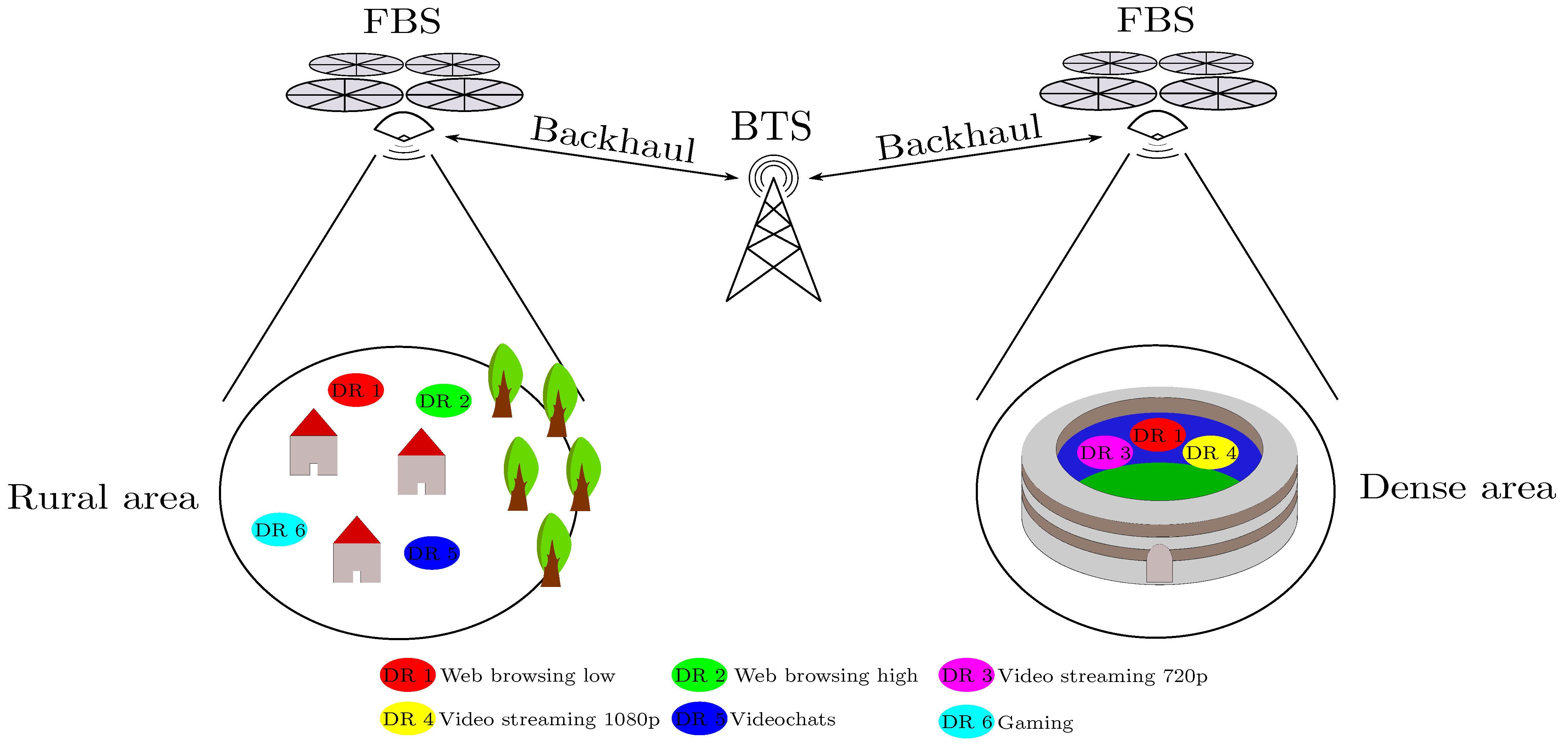
The described research follows our previous work [1], where we made a proof of the concept of the directional backhaul link for purposes of network throughput improvements in dense areas. In our work, the FBSs are used for assisting current infrastructure to extend network throughput for on-demand scenarios. The idea is demonstrated in Figure 1. There is an event with large amount of users that requires much higher network throughput than the current infrastructure can provide. The number of FBSs is determined from the users’ demand and from the available throughput from the local infrastructure. The problem described in this work is a type of coverage problem.
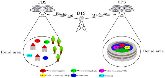
Figure 1.
Use-cases with FBSs assisting current infrastructure to extend the coverage in the area.
This paper presents a mathematical model for FBS distribution over an area. User demands and FBS throughput capacities are utilized as restricting aspects. The model is verified on a realistic music festival scenario. Heuristic algorithms were used to implement the model since its computational complexity, which is derived from the Set Covering Problem (SCP) problem is at least . It is known from the no free lunch theorem [2] that no heuristic can be considered as better than others for all the problems and their datasets. However, in the recent research on the problem of set covering-based topics the differential evolution algorithm seems promising [3]. The other promising algorithm from the available meta-heuristic algorithms is the cuckoo search that is widely used in recent literature for a wide area of optimization problems as is: (i) forest cover classification [4], (ii) load balanced data gathering [5], (iii) permutation flow shop scheduling problem [6], and many others [7,8]. For that reason, the cuckoo search and differential evolution algorithms were used including the custom modification that contains the (see Algorithm 3), to provide an efficient FBS placement.
The main contributions of this paper are as follows:
- Design of a novel model for FBS distribution over a selected area: This model is derived from SCP. Due to the high demand for data-rates, four main restricting aspects are considered, (i) user and base station capacities (for both downlink and uplink), (ii) FBS backhaul link throughput, (iii) consideration of existing base station nodes in the area to cover, (iv) the possibility to select locations with lower priority in the given area. This model provides the minimum number of required FBSs and their optimal locations. This knowledge is to be used in commercial applications;
- Implementation of two modified heuristic algorithms: differential evolution and cuckoo search were used to obtain a solution for the designed model. Differential evolution is well suited for set covering-based problems. Cuckoo search is a more recent algorithm widely used in optimization problems. Algorithms can be set for obtaining results where all users are provided with the internet coverage or the percentage of all users in case the number of FBS exceeds the maximum available limit;
- Verification of the model on real life scenario: overall feasibility of the two implemented algorithms was verified on a specific real-world scenario. Resulting number of FBSs and calculation time were used as the key performance identifiers.
2. Literature Review and State of the Art Discussion
FBSs can be utilized in a number of different use-cases, e.g., post-disaster, coverage/capacity support of local infrastructure, IoT data collection, etc. In all use-cases, the FBSs are used as an access point or relays for UEs on the ground. Depending on various parameters of the use-case, FBSs have different requirements to fulfill. Most of the research works in the topic of FBS location optimization have similar objectives with a common goal to either minimize or maximize the desired parameter in order to optimize the performance. The objectives can be summarized into two following areas:(i) maximization of UE coverage, power efficiency (endurance of UAVs), spectral efficiency, and (ii) minimization of the number of UAVs, and interferences. In our work, we focus on optimal UAV distribution over an area with the goal of minimizing the number of FBSs. This will lead to lower cost and complexity of the solution. This research can be used for both 2D and 3D FBS distribution. FBS trajectory optimization problems are not a part of the scope of this work, i.e., after FBSs are placed in the designated location, they continuously hover without moving to another location.
FBSs were discussed in numerous research works. Fotouhi et al. in [9] investigate a new mobility model for FBSs for improving the performance of cellular networks. The same authors propose, in [10], a mobility control algorithm to position FBSs to a better location to improve data throughput. In [11], Mignardi et al. propose a trajectory design of an FBS in order to improve the terrestrial base station performance. The number of studies concerning FBS increased rapidly from 2016. UAV location optimization is a problem that needs to be solved in any FBS use case. Coverage control problems of multiple UAV scenarios are discussed in [12], a review focusing on coverage methods for collective behavior of UAVs. Another review on location optimization problems was made by Cicek et al. [13] where the authors specifically target optimization methods for FBSs. To the best of author’s knowledge, these are the only two relevant overviews on this topic. According to the second overview, research studies can be divided into three main branches—static, semi-dynamic, and dynamic. Static is where UAVs and User Equipment (UE)s are stationary, semi-dynamic where UAVs can move freely but UEs are stationary, and dynamic, where UAVs and UEs can dynamically change their location. These can be further divided into scenarios with single or multiple UAVs. Our research focuses on a dynamic scenario with multiple UAVs.
UAV location can be optimized by means of different algorithms. Authors in [13] divided these algorithms into five groups: (i) exact—the algorithm is capable of finding the global optimum; (ii) well known heuristic algorithms, such as Dynamic Programming (DP), Particle Swarm Optimization (PSO), Genetic Algorithm (GA), or Gradient Algorithm (GDA); (iii) learning algorithms—these algorithms use learning procedures; (iv) enumeration—finding the best solution using exhaustive search; and (v) Problem Specific Heuristic (PSH)—a heuristic algorithm modified according to the problem properties. PSH algorithms are the most used from the list of studies, because they are most likely to give better results since they are always suited to a specific case. PSH algorithm is also used in our work, specifically Cuckoo Search (CUCKS) and Differential Evolution (DE) algorithms in modified version to serve our models.
DE is a heuristic algorithm that was developed in 1997 [14]. Differential evolution was used in many previous works for UAV path planning, e.g., in [15] the authors propose a UAV covering method with differential evolution as a cost optimization algorithm. A method for improving energy efficiency and optimize path planning was proposed in [16] and in [17]. CUCKS [18] is a relatively new algorithm introduced in 2009. It is a meta-heuristic algorithm inspired by cuckoo birds behavior. Three research works were found related to UAV distribution that used cuckoo search. In [19] the authors proposed an improved discreet cuckoo search algorithm for reconnaissance mission planning. Trajectory planning based on CUCKS was proposed in [20], where the authors focused on energy efficiency and throughput optimization. CUCKS was compared to particle swarm optimization in [21], the goal here was to evaluate online route planning methods.
In addition, the papers summarized in the overview [13], a summary of most recent papers is provided in this section, taking into account papers between the years 2018 and 2021. All papers focus on the location optimization problem with FBSs, i.e., how to optimally distribute the FBSs in order to minimize or maximize one or more parameters. Twelve papers from the past four years were selected and they are summarized in Table 1. The papers form four groups according to their goals. In the first group, the authors aim to minimize the number of required FBSs [22,23,24,25,26], in the second, to achieve maximum coverage of UEs [26,27,28,29,30], in the third, to maximize the network throughput [31,32], and, in the fourth, to maximize the spectral efficiency [33]. The optimization problem is either solved by existing algorithms or their combination [24,27,28,32,33] or a new algorithm is developed or derived from a previous algorithm [22,23,25,29,31].

Table 1.
Summary of the most recent papers on location optimization problem in FBSs use-cases.
In our research, the optimization problem is solved by the CUCKS and DE algorithms. Neither of the algorithms were used for the optimization similar to ours, i.e., minimization of the number of FBSs. The algorithms were selected as promising algorithms recently used for a wide area of optimization problems.
3. Design of Mathematical Model and Its Implementation
The effective deployment of UAV across a selected area is a difficult task. In this work, the enhancement of location covering models is presented (see Section 3.4) for the UAV deployment for on-demand connectivity scenarios. To ease the mathematical model readiness, in Table 2 we provide the terminology used in the remaining part of this paper adapted to the terms used in the literature.
Table 2.
Mapping mathematical terminology to communication networks terminology.
3.1. Deployment Model
The design of our models is based on the so-called Location Set Covering Problem (LSCP) [34] and Maximal Covering Location Problem (MCLP) [35] models from the area of facility location problems. These models have many extensions presented in the literature, however, none of these models and extensions fit into our use-case. The gap in the literature that we encounter is that the models are not considering the combination of the following factors:
- (i) each demand capacity is assigned to just one facility at a given moment;
- (ii) consideration of existing services (the capacity of existing BTS nodes in a given area must be taken into account);
- (iii) the facility capacities and demand capacities should be represented separately for downlink and uplink and not as just a number altogether because the reserved ratio for uplink and downlink may differ for each node separately;
- (iv) the possibility to select locations from the original dataset that may not be covered. This is important when we find out that to cover the whole area we need more facilities (UAVs) than is available. We can reduce the less important areas and probably save some facilities.
Implicitly we assume that the requirement of the coverage availability (distance or sufficient signal power in our case including interference consideration) from facility to demand is always met. Further in this paragraph, we reference the above-mentioned model requirements when discussing the available optimization models in the literature. The mathematical model and the need for the first requirement (i) was originally discussed in [36,37] but this need was not defined in the model, only discussed. Further, in [38], the model included that requirement. The second requirement (ii) is mathematically defined in [39] for LSCP and further extended for MCLP model in [40]. The third aspect (iii) is, to the best of our knowledge, not covered in the literature, even the recent article [41] on that topic does not consider it. The last requirement (iv) is a special version of the so-called Multi-Service Location Set Covering Problem (MS-LSCP) that is considering multiple coverages of specific demands [42] but always set to zero since the coverage requirement from the demand for a facility is always zero. Based on that, we developed a new model that targets all the above-mentioned requirements altogether.
To derive a mathematical model let us set the following notation:
- I = a set of facility sites (UAV) ;
- J = a set of demand areas (customers) ;
- = the shortest distance between facility i and demand j;
- = maximum distance which will be accepted for operation between the facilities and demands;
- = number of facilities required for servicing demand j;
- , where means that facility i is selected, while means that it is not selected;
- .
For the sake of simplicity, the facility sites will be referred as facility and demand areas as demand.
The MS-LSCP can be formulated as follows: minimize the number of facilities needed to cover the whole area, and locate them in such a manner to provide coverage for each demand by a requested number of facilities for a specific demand. In practice, this is important for back-up coverage for especially important demands to reduce the cases when some of the facilities fail and the important demand loses the connection. Formally:
Minimize
subject to
If for each demand j, then the above model is simplified to a single case, known as the classical LSCP. If then demand j does not need to be covered.
However, in real situations besides (or instead of) the MS-LSCP within the predefined range, it is more important to consider capacities of facilities. Since in our considered scenario we have to deal with the high density of users that are simultaneously connected, we assume the following additional notations:
- = capacity of facility i;
- = amount of demand at j;
- = non-fragmented demand from location j is assigned (1) or is not assigned (0) to facility i.
Further, there is a set of existing facilities (existing base station nodes in the area), and its corresponding decision variables are set to 1. Now, assume that capacities and demands are divided into uploads and downloads. For example, from the user’s point of view, the demand of 100 Mbit/s may be divided into 80 Mbit/sec for download and 20 Mbit/s for upload. To reach that expectations assume the following:
- = upload capacity of facility i;
- = download capacity of facility i;
- = upload amount of demand at j;
- = download amount of demand at j.
However, it still must be satisfied that the demand j (for download and upload at the same time) is directed to just one facility i, and the meaning of remains the same as mentioned above. Now, let us combine all these assumptions into the following model:
Minimize
subject to
where is the additional cost of building a new facility as compared to keeping an existing one. The cost cannot be easily calculated as it depends on many variables, e.g., BS location, difficulty of installation or removal, building, and law processing. The service provider must estimate this parameter for each particular location.
Since constraint (10) is non-linear, we replace it by the following equation without the product of binary variables and to obtain a mixed integer programming model.
Constraint (6) guarantees that the demand j is assigned to just one facility at a given moment. All selected facilities must have a sufficient sum of their capacities for uploads and downloads to cover all upload and download demands (in practice, this is an ideal case, network operators are trying to reach that state with the available resources). This is guaranteed by constraints (7) and (8). If a facility is selected to be removed from the network infrastructure, none of the demand should be assigned to it, this is given by constraint (9). To reduce the possible interferences we include the constraint represented by constraint (10). The is the distance between centres i and j. For all UAV pairs the distance will be greater or equal than a certain threshold that can significantly reduce the signal overlaps that usually increases the interferences.
Further, as it is typical in location covering papers where the model enhancements are presented, we provide an alternative in terms of a maximization model. This maximization model considers a predefined number of new facilities (denoted as p) to be located with the aim to cover as much as possible, denoted by p:
Maximize
subject to
3.2. Model Limitations
The proposed model has several limitations that should be addressed when adopting the model. In the following list of limitations we would like to highlight what should be improved in future research work.
- The model does not modify the FBSs’ configurations. The model uses the optimal configuration for every single FBS, however, in the final step, the FBS can modify some parameters, e.g., the transmission power to save energy or to optimize spectral efficiency. In this model, we decided not to exceed the real computation complexity of the model, because it would lead to two NP-hard problems in one model. We suggest the adopters of the model to optimize these configurations in the next processing phase. For example, the reinforcement learning techniques can be applied for optimization of the FBS’s parameters to provide a suitable solution.
- The model considers one way to reduce the interferences. In the model, the interferences can be reduced by setting the minimal distance between any two FBSs. However, the model can also include additional ways to reduce the interferences, e.g., to add another objective to find the highest distance between the BS locations;
- The model is defined for static scenarios. If the users unexpectedly change their locations, the current optimal locations have to be re-computed. In practice, it may not present a problem since the data can be prepared beforehand with suitable estimates of user requirements from the particular locations. If necessary, the computation re-run for new requirements is a task that can be run periodically, e.g., every 3, 5, 10 min, according to the requirements.
3.3. Model Computational Complexity Considerations
The size of the search space is determined by the number of all possible selections of facilities. For m facilities, according to the binomial theorem, it is equal to
Furthermore, we need to find the most complex condition in extended models for (where n is the number of demand areas) to find the resulting computational complexity. In the minimization model these are constraint (9), and (13) in the corresponding constraints of the maximization model, which require operations. Based on that the resulting time complexity of these models is .
3.4. Designated Implementation
The mathematical model from the Section 3.1, enhancing the LSCP and MCLP models that are originally evolved from SCP, falls into class of problems. In this section, we proposed the implementation of a designed model presented in constraints (4) to Equation (13) using two heuristic algorithms that ease the integration and reproducibility of the proposed solution into a software solution that may use them.
Since the original model SCP is , it is suitable to employ heuristic algorithms to solve such tasks for larger datasets (more than 55-60 UAVs), to reach a solution in a reasonable time. For the UAV deployment use-case of this paper, two promising meta-heuristic algorithms were chosen. First, the CUCKS algorithm with Lévy Flights [43,44], and the DE [15,45], that can provide a suitable solution for this problem.
The CUCKS algorithm pseudocode used to generate a feasible solution (defined by the network designer for a given use-case, e.g., a solution that contains less than x UAVs to cover the selected area with the given requirements) is shown in Algorithm 1.
| Algorithm 1 Cuckoo search for UAV deployment pseudocode |
| Input: τ terminal condition, e.g., number of iterations |
|
The CUCKS algorithm first generates the initial population of n host nests. This, in technical terminology, means that it randomly generates the particular solutions for UAV deployment. The solution is represented by the combination of UAV locations for the deployment. Then, the algorithm evaluates each individual solution by the fitness function. That is defined based on the objective function presented in term (4) as follows:
where n is the number of host nests and represents the state if the UAV device was considered in the solution, 1 if it was and 0 if it was not.
Then, the Algorithm 2 on line six checks if the randomly generated nests in the solution contain the feasible solution. If not, the algorithm works as a standard cuckoo search algorithm with one modification, which is the application of the so-called described in more detail below in this section.
Further, we use the DE algorithm to compare the different heuristics to generate a feasible solution. The DE algorithm uses the same objective function as in the case of the cuckoo search algorithm (sum (27)), however, it does use individuals instead of nests. The DE algorithm first generates the initial population of n individuals and in a loop provides the standard flow of DE with a modification of the application. This is applied before the algorithm inserts the newly generated individuals (after the selection, mutation, and other operations succeeded) into the actual population. The whole DE algorithm to generate a feasible solution is shown in Algorithm 2.
| Algorithm 2 Differential evolution for UAV deployment pseudocode |
| Input: τ terminal condition, e.g., the number of iterations; |
|
is used in both algorithms. Here, the usage of is essential since the solution generated by CUCKS and DE can provide an infeasible solution (a solution that would not cover customers based on the given requirements). For that reason, the repair operator function was designed for modification of the solution provided by both algorithms and changes it to a feasible solution for a given use-case.
The designed repair operator is shown in Algorithm 3. The algorithm sequentially traverses each aspect of the model and adds services to meet that aspect. After going through all aspects of the model (customer availability, capacity, multiple services) it can be said that all the conditions defined by the model are met and the solution to the problem is valid.
| Algorithm 3 Repair operator for both heuristics |
| Input: = the set of all facilities; |
|
4. Model Verification
The presented model from Section 3.1 is targeted at specific scenarios that are characterized by a high number of users (tens of thousands) spread over large outdoor areas. In other words, scenarios, where multiple UAVs are necessary to cover the area, are expected. The more UAVs are needed the more complex the problem is, and the more beneficial our model becomes. Model definition does not depend on the number of users and UAVs, however the implementation, i.e., the designed algorithms does. To verify that our model is valid and gives realistic and valuable results, it is important to simulate it in a specific scenario. This model was verified on a real outdoor music festival scenario described in Section 4.1. The numerical results are discussed further in Section 4.2.
4.1. Scenario Description
The music festival is located on an airstrip of size 2000 by 500 m, however the occupied area by the festival is only 1270 by 400 m with an additional parking area in top left corner of size 70 by 240 m. This considered area of small airstrip is located near Milovice, Czech Republic (GPS coordinates: 50°1410.5 N 14°5515.2 E) which was built in around 1922. In past, it was a military airfield, later it served as an airfield for small aeroclubs. Nowadays, it only hosts a few public events per year and is not used as an airfield anymore, also due to the bad runway condition. The surface is flat and there are no buildings and trees inside the area. This area can host more than one hundred thousand people, but in the past years the usual attendance was between 50 and 80 thousand people per event. The airfield is located in a rural area with a few villages nearby which means that the local telecommunication infrastructure is not prepared for tens of thousands of connections with high throughput demand so the coverage for these events is usually boosted by cells on wheels.
Our scenario estimates 70 thousand attendees. This is a rounded mean value of published numbers of attendees between the years 2007 and 2017. It is the total value of attendees throughout the whole four-day event, this means that the number of attendees at each moment will be lower and will fluctuate. The attendees are divided into seven groups with respect to their capacity requirements. The division was inspired by the example of the traffic model from [46]. The traffic mix was modified according to our estimation in our music festival scenario. It is also estimated, that 50% of users will not be using the internet for various reasons, e.g., sleeping, eating, relaxing, enjoying the festival. The other 50% will be using a mix of traffic shown in Table 3. Percentage of users represents the percentage from all participating users during the festival, Number of users the percentage of users translated into specific number of users, and required capacity the data-rate capacity required by a single user. Aforementioned values were estimated by the authors and are not based on any statistics or studies.
Table 3.
Traffic mix distribution among users.
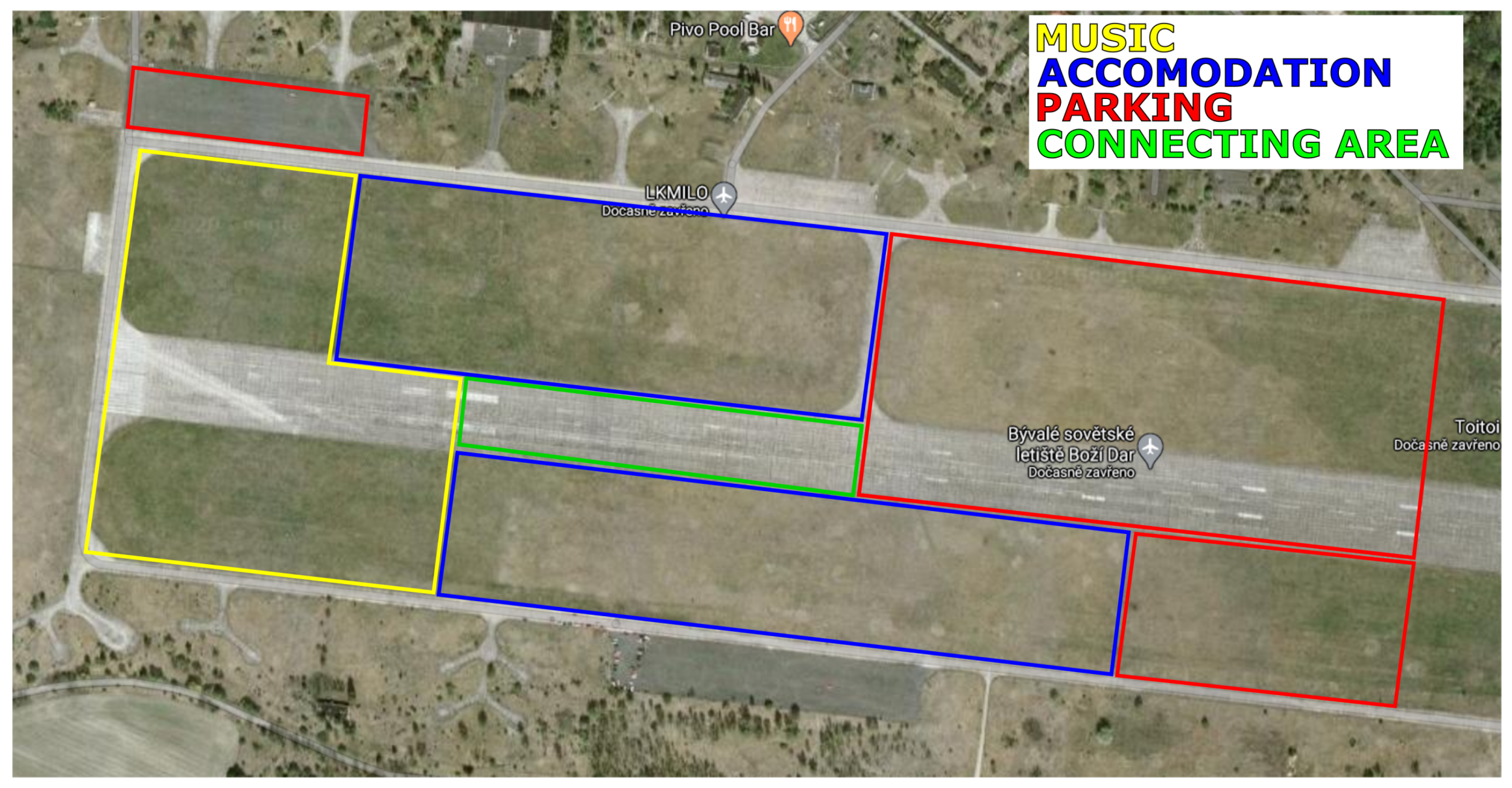
The area is divided into several sub-areas, as shown in Figure 2. Each sub-area has its own purpose, i.e., music, accommodation, parking, common area. The common area works as a connecting point for all other areas, also usually the food stands are located here. According to their purposes, each subarea was assigned a specific user density. Subarea sizes with numbers of users and user densities are shown in Table 4. Users in each subareas are distributed uniformly, 60% of all users are placed into the music area. It is the area where most of the people are gathering. 30% of users are likely in the accommodation and common area, and the last portion of 10% is located in the parking area. For summarizing, the scenario parameters are shown in Table 5.
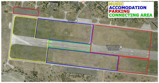
Figure 2.
Real satellite photo of the airfield with marked subareas.
Table 4.
Subarea division with user densities.
Table 5.
Scenario parameters.
The FBSs in our scenario play the role of relays. This means that they receive signal from users and transmit it to the internet or the other way round. The wireless equipment can be then divided into two parts, backhaul—connection between FBS and nearby BS, and service—connection between FBS and users. This paper does not concentrate on the backhaul link and it is considered to be ideal and with no throughput limit. The throughput limits are however applied on the service link. There are number of factors that determine the available throughput of the access link, e.g., technology limitations, technology setup—proper antenna alignment, position, and direction, medium limitations—interference.
The FBSs in our scenario are supposed to augment terrestrial BS. However, their design in terms of access link must be slightly modified. The terrestrial BSs expect to serve the users in higher distances, usually higher than 500 m in case of rural area. Additionally, the users are not expected to be located in the close vicinity of the BS (within the radius of one to three hundred meters) and overflowing with thousands of people. However, in case of the FBSs, it is placed directly above the user clusters. For these reasons, the wireless part of the service link must be redesigned. Currently, there are two technologies worth considering for our scenario. FBSs are quite constrained in terms of payload which leads us to consider the IEEE 802.11ac and IEEE 802.11ad, technologies capable of lightweight implementations. The first standard is very well used in many personal and industrial use cases. It is a quite reliable and powerful standard capable of providing a theoretical PHY data-rate of 6933 Mb/s with 4 × 4 MIMO [47]. The second is not so widely utilized but has interesting perspectives with the theoretical PHY data-rate of 6756.75 Mb/s on a single stream [48]. These values are however not realistic in live scenarios. Not all available devices are capable of providing such high MIMO capabilities and it is not likely that the channel conditions will be good in distances over 50 m. In addition to that, current available devices are usually limited on the other side by 1 Gb/s Ethernet cable. Additionally, it is important to note that PHY data-rate is not what the end user receives and the data-rate on the application layer is more suitable. It is estimated that the usual drop between physical and application layer can be typically between 20% and 30%, adding another 20 to 30% loss due to the channel conditions, then the more realistic data-rate on the service side would be around 3 Gb/s. This value was selected as the service link limit for each FBS.
There are two cell towers in the nearest area, both of them with LTE capabilities. The two towers combined provide coverage for all three operators in the Czech Republic. According to [49], typical data-rates for each LTE BS is 1 Gb/s uplink and 500 Mb/s downlink. This would mean that the total of 4.5 Gb/s could be theoretically available from the local infrastructure. The total data-rate requirements for all users in our scenario is 29,610 Mb/s. The local cell towers could then cover roughly 15% of the demand. However, since there is also a demand from local villages, it is not possible to be sure of the cell towers availability and for this reason the local infrastructure is neglected from the calculations. The data about cell towers were obtained from [50].
4.2. Numerical Results and Discussions
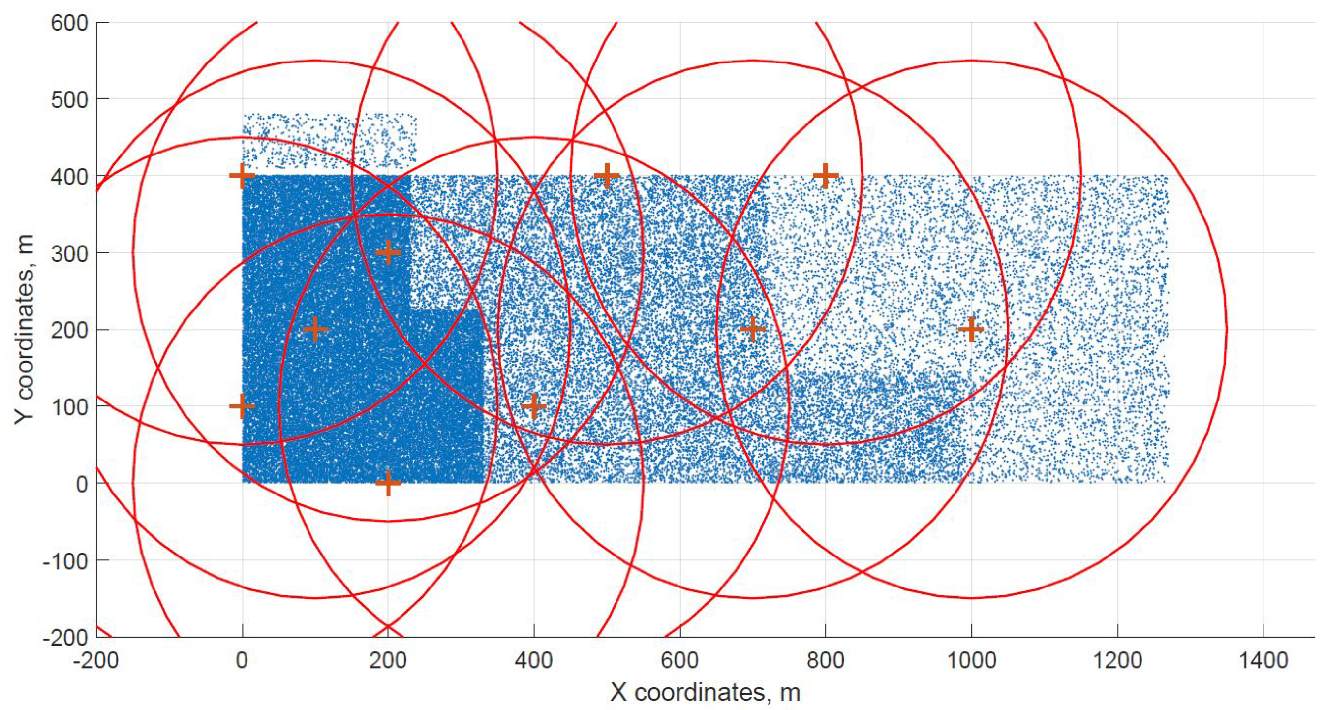
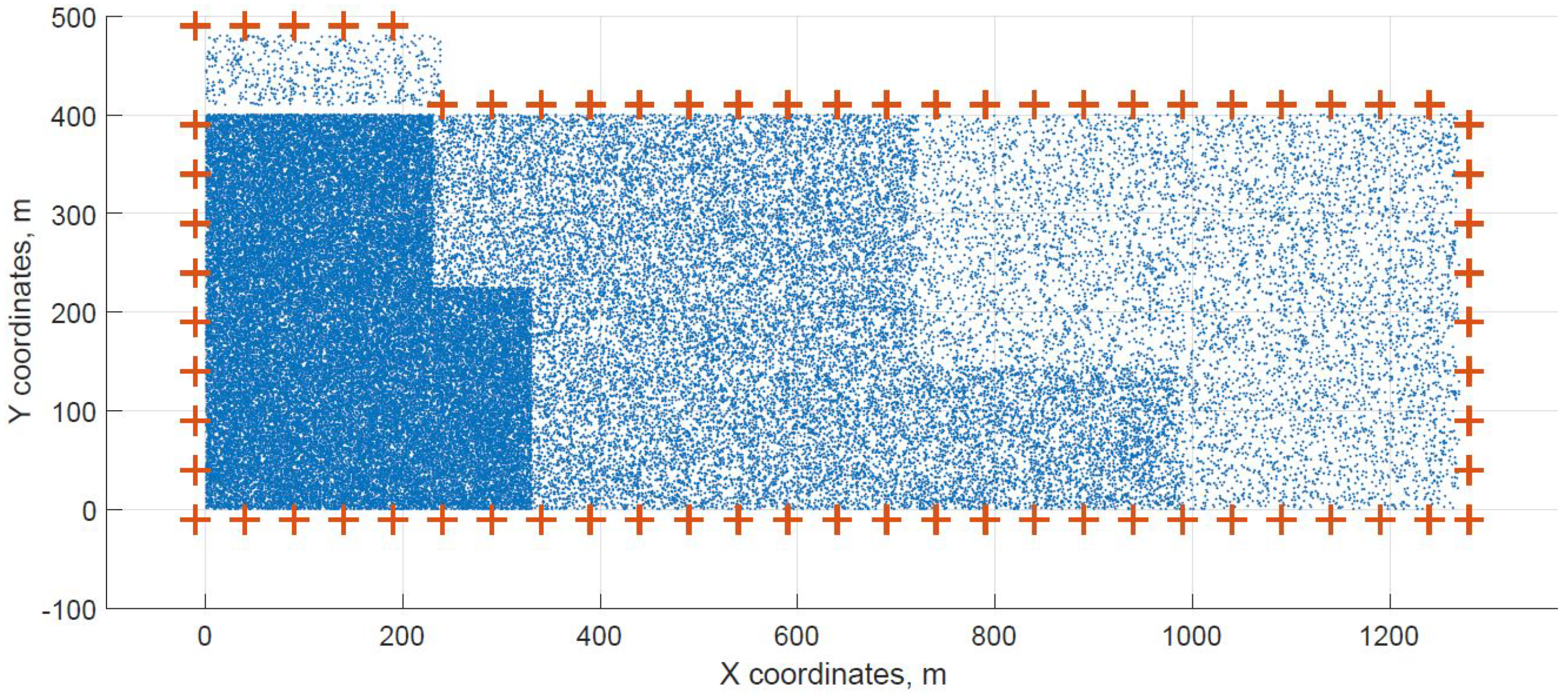
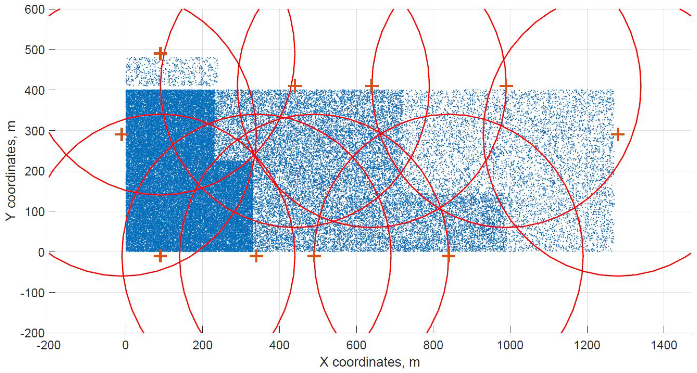
For a demonstration, two datasets (C and G) are visualized in this section. The original distribution of FBSs for dataset C is shown in Figure 3 with the results shown in Figure 4 and Figure 5. In case of dataset G, the original distribution of FBSs is shown in Figure 6 with the corresponding results in Figure 7 and Figure 8. Small blue dots symbolize users, different densities are clearly visible. Red crosses symbolize potential locations for placing FBSs. Red circles show the radii of each FBS. The radii are not visualized in Figure 3 and Figure 6 for the picture to stay clear. The whole process of data generation and processing consisted of three major steps. First, the two original distributions of FBS were generated, as well as the distribution of users. Each FBS and each user has unique coordinates in the area. Second, the data from the first step were passed to the two algorithms for calculation. Third, the output data from the algorithms were visualized by the same code as in the first step. MATLAB tool was used in steps one and three. Step two was implemented in OpenJDK without any specific external library.
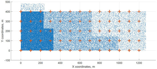
Figure 3.
Original distribution grid with FBSs placed inside of the area for dataset C.
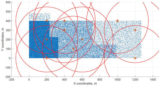
Figure 4.
Cuckoo search resulting grid for dataset C.

Figure 5.
Differential evolution resulting grid for dataset C.
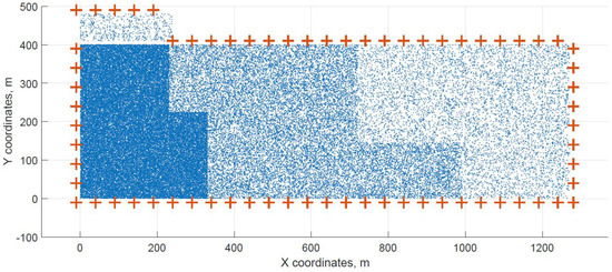
Figure 6.
Original distribution with users outside of the area for dataset G.
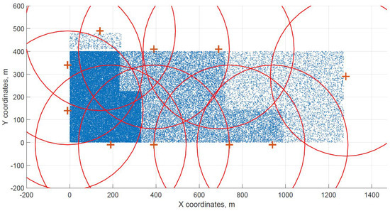
Figure 7.
Cuckoo search resulting grid for dataset G.

Figure 8.
Differential evolution resulting grid for dataset G.
The number of possible solutions is high and a reasonably good solution had to be selected. The input data consisted of eight datasets named by capital letters from A to H. A total of sixteen simulations were run, eight simulations per each algorithm. The results were selected based on the number of FBSs needed for the deployment, in our case the smaller number the better. When two results had the same number of FBSs, the solution taking less computation time was selected. The computation was performed on a personal computer with parameters described in Table 6. Ten thousand iterations were performed for each algorithm. In these runs, the resulting number of FBSs varied from the best result to plus one or two more locations. The results are shown in Table 7.
Table 6.
Testing environment parameters.
Table 7.
Calculation results for CUCKS and DE algorithms using 10,000 iterations.
Two cases of FBS deployment were investigated, one where FBSs are distributed evenly in a grid inside the whole area and second where the FBSs are also distributed evenly but on the edges of the area. The second deployment was investigated for cases when FBSs are not allowed to fly over crowded areas for safety reasons. The original distribution of the first case for dataset C is shown in Figure 3, the FBSs are deployed in a grid with distances of 100 m. This lead to the total number of 70 initial deployment locations. The initial locations of the second case for dataset G are shown in Figure 6. Here, the distances between FBSs were shortened to 50 m to reach similar number of original locations as in case one. The number of initial locations plays a big role in calculation time of the minimized solution. According to the results from Table 7, it was proven that numbers between 60 and 70 symbolize a certain threshold for calculation complexity, because for the datasets D and H where the numbers of initial locations were 90 and 85 prolonged the calculation time radically. Longer time would compromise the usefulness of the algorithms for repeated use in short periods of time, for instance in case of high user mobility. On the other hand, it would make the result more accurate.
The processing of the algorithms takes certain amount of time. Specifically for datasets C and G, processing of the CUCKS took 2274 s for the case with the BS inside of the area and 1856 s for the BS outside of the area. These values are approximately four to six times higher than those for DE: 373 s for the case with the BS inside of the area and 387 s for the BS outside of the area. The number of resulting locations in all four cases was ten. The reason for this was likely that the required average data-rate of all users combined at each moment was 29,610 Mb/s. If this value is divided by the available throughput on each FBS (3 Gb/s), we achieve ten. This means that the resulting number of locations is highly affected by the throughput limit of the FBSs rather than by the radius of their wireless devices.
The distribution of FBSs seems logical for both algorithms and both cases. The algorithms validate the expected result that more locations will be selected over areas with higher user densities. It is visible more in the cases with locations inside of the area, i.e., Figure 4 and Figure 5. Clearly, the user density forces the algorithms to select more locations in the denser areas. Both algorithms give similar results in terms of FBS distribution, however if the preference was the calculation time, the DE should be the favorable option. The shorter calculation time would be appreciated in scenarios where the FBSs’ position would be constantly updated. The reason why DE is so much faster than CUCKS is that the DE algorithm is not generating the new pool of solutions for each generation in opposite to the CUCKS algorithm.
The data-rate and radius parameters used in the scenario were derived from theoretical capabilities of two technologies—IEEE 802.11ac and IEEE 802.11ad. Even though the results support the theoretical values, it is difficult to predict the outcome of a real implementation because there are still a great number of variables during live test, e.g., weather conditions, inter-BS and inter-user interference, and rapid user mobility. That means, real measurements are required to support the theoretical values. Even though the measurements would show much lower performance, future of mmWave communications might provide even greater and more stable parameters with the new IEEE 802.11ay standard. It is an updated IEEE 802.11ad standard promising extended range and higher throughput provided by newly implemented multiple-input and multiple-output (MIMO) feature.
Let us now discuss the limitations of used methods in this research. The limitations lie in the initial number of FBSs locations, since increasing this number would extend dramatically the calculation time. As it was established for our case, this would not be such a critical issue because of the high number of users in the area. In some other cases however, it might be crucial to position the FBSs into more precise spots. Further, in our scenario, there is theoretically unlimited number of FBSs available to cover the area. If the user requirements would rise or if the FBS capabilities would be lower, the number of FBSs could rise to the point where the total implementation price would make the solution unfeasible. This condition can be implemented in the algorithm, however it is not for the reason that authors wanted to keep the decision making under their control.
For future research directions we expect to implement and verify more heuristic algorithms and also provide additional models targeting a situation in which there is a specific number of drones (significantly limited resources). The focus will be more on how to cover as most as possible locations using the optimized heuristic parameters, with a detailed focus on scenarios where the users are quickly moving to different locations.
One of the important factors to be considered is both inter-BS and inter-user interference. Including interference reduction into described algorithms would radically increase complexity of the solution in the way that it would become even more difficult to obtain a solution with regards to calculation time and computational complexity. One option to address the interferences problem is in the next stage after obtaining the solution from the algorithms. This is planned as the next step in this research. There are various approaches to address the interference problem from which the following approaches are planned by the authors:
- Setting minimum distance from one FBS to another;
- Using mathematical model with multi-objective function–minimize number of FBSs and maximize distance between BSs;
- Reducing radius of the FBSs by reducing antenna gain;
- Using different radio frequencies among neighboring FBSs.
5. Conclusions
The key objective of this paper was the optimal FBS distribution over a desired area while minimizing the number of necessary FBSs. Two novel mathematical models were designed for this purpose. The models take into account several aspects that are crucial in the presented scenario. It includes the capacities for both downlink and uplink, the consideration of existing base station nodes in the UAV deployment area, and the possibility to select lower priority locations that may be excluded from the coverage. Further, we consider the computational complexity of these models for very large datasets, which are defined by tens of thousands of users and tens of FBSs. We employ cuckoo search and differential evolution algorithms with the developed providing a feasible solution to this problem.
To verify the viability of the models, data from a real-life scenario were used. The Presented scenario was a crowded music festival with various user densities. Two use-cases for FBS distribution were tested. First with FBSs distributed inside the area and second with FBSs outside the area. The two algorithms were implemented and the optimal solution was obtained via extensive simulations with eight datasets. Both of the algorithms were able to find a solution. Major difference was in the computation time where the CUCKS obtained results in time three to six times higher for the two use-cases than the DE. It is however important to consider that even though the higher number of candidate locations can provide higher accuracy of the final solution, it can lead to unnecessary waiting time. It is recommended for future model adopters to find an optimal number of the candidate locations suitable for their specific use-case.
The data used as inputs for the implemented algorithms were mostly based on theoretical values, and the research would benefit greatly from support of real-life measurements. The measurements might reveal some deficiency in data-rates and FBSs’ radii. One cause of the deficiency might be signal interferences, that have not been addressed in this research. However, as discussed in Section 4.2, including interferences might make our models excessively complex, hence the issue of interferences will be addressed in detail in our future research.
Author Contributions
Conceptualization, J.P., P.S., J.H; methodology, J.P., P.S.; software, J.P., P.S.; validation, J.P., P.S., M.S.; formal analysis, P.S.; data curation, J.P., P.S., M.S.; writing—original draft preparation, J.P., P.S.; writing—review and editing, J.H; visualization, J.P.; supervision, M.S., J.H. All authors have read and agreed to the published version of the manuscript.
Funding
The described research was financed by the Ministry of Industry and Trade of Czech Republic project No. FV40309.
Institutional Review Board Statement
Not applicable.
Informed Consent Statement
Not applicable.
Data Availability Statement
Not applicable.
Conflicts of Interest
The authors declare no conflict of interest.
References
- Gerasimenko, M.; Pokorny, J.; Schneider, T.; Sirjov, J.; Andreev, S.; Hosek, J. Prototyping Directional UAV-Based Wireless Access and Backhaul Systems. In Proceedings of the 2019 IEEE Global Communications Conference (GLOBECOM), Big Island, HI, USA, 9–13 December 2019; IEEE: Piscataway, NJ, USA, 2019; pp. 1–6. [Google Scholar]
- Wolpert, D.H.; Macready, W.G. No free lunch theorems for optimization. IEEE Trans. Evol. Comput. 1997, 1, 67–82. [Google Scholar] [CrossRef] [Green Version]
- Kritter, J.; Brévilliers, M.; Lepagnot, J.; Idoumghar, L. On the optimal placement of cameras for surveillance and the underlying set cover problem. Appl. Soft Comput. 2019, 74, 133–153. [Google Scholar] [CrossRef]
- Shanthasheela, A.; Shanmugavadivu, P. Cuckoo Search Based Forest Cover Classification. J. Comput. Theor. Nanosci. 2019, 16, 3550–3553. [Google Scholar] [CrossRef]
- Sadeghi, F.; Avokh, A. Load-balanced data gathering in Internet of Things using an energy-aware cuckoo-search algorithm. Int. J. Commun. Syst. 2020, 33, e4385. [Google Scholar] [CrossRef]
- Zhang, Y.; Yu, Y.; Zhang, S.; Luo, Y.; Zhang, L. Ant colony optimization for Cuckoo Search algorithm for permutation flow shop scheduling problem. Syst. Sci. Control. Eng. 2019, 7, 20–27. [Google Scholar] [CrossRef]
- Thirugnanasambandam, K.; Prakash, S.; Subramanian, V.; Pothula, S.; Thirumal, V. Reinforced cuckoo search algorithm-based multimodal optimization. Appl. Intell. 2019, 49, 2059–2083. [Google Scholar] [CrossRef]
- Cai, X.; Niu, Y.; Geng, S.; Zhang, J.; Cui, Z.; Li, J.; Chen, J. An under-sampled software defect prediction method based on hybrid multi-objective cuckoo search. Concurr. Comput. Pract. Exp. 2020, 32, e5478. [Google Scholar] [CrossRef]
- Fotouhi, A.; Ding, M.; Hassan, M. Service on demand: Drone base stations cruising in the cellular network. In Proceedings of the 2017 IEEE Globecom Workshops (GC Wkshps), Singapore, 4–8 December 2017; IEEE: Piscataway, NJ, USA, 2017; pp. 1–6. [Google Scholar]
- Fotouhi, A.; Ding, M.; Hassan, M. Flying drone base stations for macro hotspots. IEEE Access 2018, 6, 19530–19539. [Google Scholar] [CrossRef]
- Mignardi, S.; Verdone, R. On the performance improvement of a cellular network supported by an unmanned aerial base station. In Proceedings of the 2017 29th International Teletraffic Congress (ITC 29), Genoa, Italy, 4–8 September 2017; IEEE: Piscataway, NJ, USA, 2017; Volume 2, pp. 7–12. [Google Scholar]
- Huang, S.; Teo, R.S.H.; Leong, W.L.; Martinel, N.; Forest, G.L.; Micheloni, C. Coverage Control of Multi-Unmanned Aerial Vehicles: A Short Review. Unmanned Syst. 2018, 6, 1–14. [Google Scholar]
- Cicek, C.T.; Gultekin, H.; Tavli, B.; Yanikomeroglu, H. UAV base station location optimization for next generation wireless networks: Overview and future research directions. In Proceedings of the 2019 1st International Conference on Unmanned Vehicle Systems-Oman (UVS), Muscat, Oman, 5–7 February 2019; IEEE: Piscataway, NJ, USA, 2019; pp. 1–6. [Google Scholar]
- Storn, R.; Price, K. Differential evolution—A simple and efficient heuristic for global optimization over continuous spaces. J. Glob. Optim. 1997, 11, 341–359. [Google Scholar] [CrossRef]
- Gonzalez, V.; Monje, C.A.; Garrido, S.; Moreno, L.; Balaguer, C. Coverage Mission for UAVs Using Differential Evolution and Fast Marching Square Methods. IEEE Aerosp. Electron. Syst. Mag. 2020, 35, 18–29. [Google Scholar] [CrossRef]
- Wang, Z.; Liu, R.; Liu, Q.; Thompson, J.S.; Kadoch, M. Energy Efficient Data Collection and Device Positioning in UAV-Assisted IoT. IEEE Internet Things J. 2019, 7, 1122–1139. [Google Scholar] [CrossRef]
- Adhikari, D.; Kim, E.; Reza, H. A fuzzy adaptive differential evolution for multi-objective 3D UAV path optimization. In Proceedings of the 2017 IEEE Congress on Evolutionary Computation (CEC), San Sebastián, Spain, 5–8 June 2017; IEEE: Piscataway, NJ, USA, 2017; pp. 2258–2265. [Google Scholar]
- Yang, X.S.; Deb, S. Cuckoo search via Lévy flights. In Proceedings of the 2009 World Congress on Nature & Biologically Inspired Computing (NaBIC), Coimbatore, India, 9–11 December 2009; IEEE: Piscataway, NJ, USA, 2009; pp. 210–214. [Google Scholar]
- Zhang, Y.Z.; Li, H.; Ma, Y.H.; Zhang, J.D.; He, J.L. Cooperative reconnaissance mission planning for heterogeneous UAVs with DCSA. In Proceedings of the 2019 IEEE 15th International Conference on Control and Automation (ICCA), Edinburgh, UK, 16–19 July 2019; IEEE: Piscataway, NJ, USA, 2019; pp. 417–422. [Google Scholar]
- Zhu, K.; Xu, X.; Han, S. Energy-efficient UAV trajectory planning for data collection and computation in mMTC networks. In Proceedings of the 2018 IEEE Globecom Workshops (GC Wkshps), Abu Dhabi, UAE, 9–13 December 2018; IEEE: Piscataway, NJ, USA, 2018; pp. 1–6. [Google Scholar]
- Góez-Sánchez, G.D.; Jaramillo-Garzón, J.A.; Velásquez, R.A. Performance comparison of particle swarm optimization and Cuckoo search for online route planning. IEEE Aerosp. Electron. Syst. Mag. 2018, 33, 40–50. [Google Scholar] [CrossRef]
- Zhang, S.; Sun, X.; Ansari, N. Placing multiple drone base stations in hotspots. In Proceedings of the 2018 IEEE 39th Sarnoff Symposium, Newark, NJ, USA, 24–25 September 2018; IEEE: Piscataway, NJ, USA, 2018; pp. 1–6. [Google Scholar]
- Qin, J.; Wei, Z.; Qiu, C.; Feng, Z. Edge-Prior Placement Algorithm for UAV-Mounted Base Stations. In Proceedings of the 2019 IEEE Wireless Communications and Networking Conference (WCNC), Marrakech, Morocco, 15–18 April 2019; IEEE: Piscataway, NJ, USA, 2019; pp. 1–6. [Google Scholar]
- Wang, H.; Zhao, H.; Wu, W.; Xiong, J.; Ma, D.; Wei, J. Deployment algorithms of flying base stations: 5G and beyond with UAVs. IEEE Internet Things J. 2019, 6, 10009–10027. [Google Scholar] [CrossRef]
- Sivalingam, T.; Manosha, K.S.; Rajatheva, N.; Latva-aho, M.; Dissanayake, M.B. Positioning of Multiple Unmanned Aerial Vehicle Base Stations in future Wireless Network. In Proceedings of the 2020 IEEE 91st Vehicular Technology Conference (VTC2020-Spring), Antwerp, Belgium, 25–28 May 2020; IEEE: Piscataway, NJ, USA, 2020; pp. 1–6. [Google Scholar]
- Zhao, H.; Wang, H.; Wu, W.; Wei, J. Deployment algorithms for UAV airborne networks toward on-demand coverage. IEEE J. Sel. Areas Commun. 2018, 36, 2015–2031. [Google Scholar] [CrossRef]
- Chen, Y.; Li, N.; Wang, C.; Xie, W.; Xv, J. A 3D placement of unmanned aerial vehicle base station based on multi-population genetic algorithm for maximizing users with different QoS requirements. In Proceedings of the 2018 IEEE 18th International Conference on Communication Technology (ICCT), Chongqing, China, 8–11 October 2018; IEEE: Piscataway, NJ, USA, 2018; pp. 967–972. [Google Scholar]
- Sun, J.; Masouros, C. Deployment strategies of multiple aerial BSs for user coverage and power efficiency maximization. IEEE Trans. Commun. 2018, 67, 2981–2994. [Google Scholar] [CrossRef] [Green Version]
- Lai, C.C.; Chen, C.T.; Wang, L.C. On-demand density-aware UAV base station 3D placement for arbitrarily distributed users with guaranteed data rates. IEEE Wirel. Commun. Lett. 2019, 8, 913–916. [Google Scholar] [CrossRef] [Green Version]
- Adam, N.; Tapparello, C.; Heinzelman, W.; Yanikomeroglu, H. Placement optimization of multiple UAV base stations. In Proceedings of the 2021 IEEE Wireless Communications and Networking Conference (WCNC), Nanjing, China, 29 March 2021; IEEE: Piscataway, NJ, USA, 2021; pp. 1–7. [Google Scholar]
- Becvar, Z.; Mach, P.; Plachy, J.; de Tudela, M.F.P. Positioning of Flying Base Stations to Optimize Throughput and Energy Consumption of Mobile Devices. In Proceedings of the 2019 IEEE 89th Vehicular Technology Conference (VTC2019-Spring), Kuala Lumpur, Malaysia, 28 April–1 May 2019; IEEE: Piscataway, NJ, USA, 2019; pp. 1–7. [Google Scholar]
- Li, J.; Lu, D.; Zhang, G.; Tian, J.; Pang, Y. Post-Disaster Unmanned Aerial Vehicle Base Station Deployment Method Based on Artificial Bee Colony Algorithm. IEEE Access 2019, 7, 168327–168336. [Google Scholar] [CrossRef]
- Hydher, H.; Jayakody, D.N.K.; Hemachandra, K.T.; Samarasinghe, T. Intelligent UAV deployment for a disaster-resilient wireless network. Sensors 2020, 20, 6140. [Google Scholar] [CrossRef]
- ReVelle, C.; Toregas, C.; Falkson, L. Applications of the location set-covering problem. Geogr. Anal. 1976, 8, 65–76. [Google Scholar] [CrossRef]
- Church, R.; ReVelle, C. The maximal covering location problem. Pap. Reg. Sci. 1974, 32, 101–118. [Google Scholar] [CrossRef]
- Current, J.R.; Storbeck, J.E. Capacitated covering models. Environ. Plan. B Plan. Des. 1988, 15, 153–163. [Google Scholar] [CrossRef]
- Gerrard, R.A. The Location of Service Facilities Using Models Sensitive to Response Distance, Facility Workload, and Demand Allocation. Ph.D. Thesis, University of California, Santa Barbara, CA, USA, 1995. [Google Scholar]
- Seda, P.; Seda, M.; Hosek, J. On Mathematical Modelling of Automated Coverage Optimization in Wireless 5G and beyond Deployments. Appl. Sci. 2020, 10, 8853. [Google Scholar] [CrossRef]
- Plane, D.R.; Hendrick, T.E. Mathematical programming and the location of fire companies for the Denver fire department. Oper. Res. 1977, 25, 563–578. [Google Scholar] [CrossRef]
- Murray, A.T. Optimising the spatial location of urban fire stations. Fire Saf. J. 2013, 62, 64–71. [Google Scholar] [CrossRef]
- Chauhan, D.; Unnikrishnan, A.; Figliozzi, M. Maximum coverage capacitated facility location problem with range constrained drones. Transp. Res. Part C Emerg. Technol. 2019, 99, 1–18. [Google Scholar] [CrossRef]
- Church, R.L.; Gerrard, R.A. The multi-level location set covering model. Geogr. Anal. 2003, 35, 277–289. [Google Scholar] [CrossRef]
- Yang, W.; Yang, H.; Tang, S. Optimization and control application of sensor placement in aeroservoelastic of UAV. Aerosp. Sci. Technol. 2019, 85, 61–74. [Google Scholar] [CrossRef]
- Song, P.C.; Pan, J.S.; Chu, S.C. A parallel compact cuckoo search algorithm for three-dimensional path planning. Appl. Soft Comput. 2020, 94, 106443. [Google Scholar] [CrossRef]
- Huang, P.Q.; Wang, Y.; Wang, K.; Yang, K. Differential Evolution With a Variable Population Size for Deployment Optimization in a UAV-Assisted IoT Data Collection System. IEEE Trans. Emerg. Top. Comput. Intell. 2019, 4, 324–335. [Google Scholar] [CrossRef]
- Alliance, N. Radio access performance evaluation methodology. NGMN White Pap. 2008, 1, 36. [Google Scholar]
- Rochim, A.F.; Harijadi, B.; Purbanugraha, Y.P.; Fuad, S.; Nugroho, K.A. Performance comparison of wireless protocol IEEE 802. In 11 ax vs 802.11 ac. In Proceedings of the 2020 International Conference on Smart Technology and Applications (ICoSTA), Surabaya, Indonesia, 20 February 2020; IEEE: Piscataway, NJ, USA, 2020; pp. 1–5. [Google Scholar]
- Zhu, X.; Doufexi, A.; Kocak, T. Throughput and coverage performance for IEEE 802.11 ad millimeter-wave WPANs. In Proceedings of the 2011 IEEE 73rd Vehicular Technology Conference (VTC Spring), Budapest, Hungary, 15–18 May 2011; IEEE: Piscataway, NJ, USA, 2011; pp. 1–5. [Google Scholar]
- 3GPP. Requirements for Further Advancements for Evolved Universal Terrestrial Radio Access (E-UTRA) (LTE-Advanced); Technical Report (TR) 36.913; Version 15.0.0; 3rd Generation Partnership Project (3GPP): Valbonne, France, 2018. [Google Scholar]
- Hornyák, J.; Skřivánek, P.; Mikuláštík, K.; Radek, Z. Interactive Map of Deployed BTS in Czech Republic. Available online: http://gsmweb.cz/ (accessed on 30 June 2021).


Publisher’s Note: MDPI stays neutral with regard to jurisdictional claims in published maps and institutional affiliations. |
© 2021 by the authors. Licensee MDPI, Basel, Switzerland. This article is an open access article distributed under the terms and conditions of the Creative Commons Attribution (CC BY) license (https://creativecommons.org/licenses/by/4.0/).