1. Introduction
Owing to an increase in the number of portable devices, such as mobile phones and tablets, over the past few years [
1,
2], an increasing number of indoor location-based services [
3], including navigation, location-based social networking, and motion tracking have attracted more and more attention over time. Unlike the outdoor environment, where the global positioning system (GPS) can provide accurate localization using line-of-sight signals, the indoor positioning system based on GPS significantly degrades because of signal attenuation through the building’s walls [
4]. Compared to GPS signals, Wi-Fi signals are more stable in indoor environments because of their wide deployment and easy access; thus, the utilization of Wi-Fi signals to achieve accurate indoor localization has recently gained significant interest [
5].
As a state-of-the-art technology, Wi-Fi fingerprinting indoor localization systems (IPS) have been extensively researched for both localization [
6,
7] and activity recognition [
8,
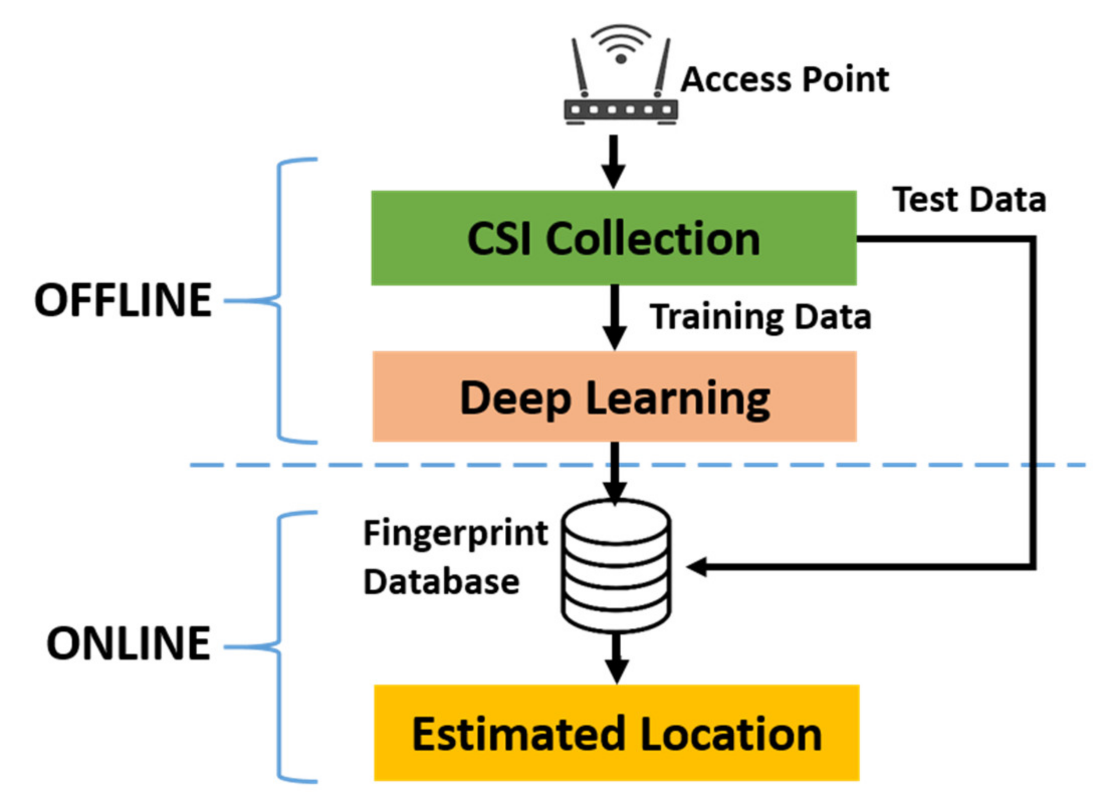
9] applications. As the radio frequency (RF) characteristics of Wi-Fi signals at each location are unique due to their different propagation paths, the RF characteristics can be considered unique fingerprints. With all the fingerprints of locations collected and stored in the database beforehand, an accurate localization can be achieved by comparing the received Wi-Fi signal with the data in the database.
A Wi-Fi fingerprinting IPS can utilize either the received system strength indicator (RSSI) or channel state information (CSI) as fingerprints for each location. For Wi-Fi-based IPSs using RSSI, ref. [
10] demonstrated that an RSSI heat map can be used to estimate the target location by applying the overlap technique to RSSI heat maps of access points (APs). The heat maps generated for both line-of-sight and non-line-of-sight (NLOS) path loss models for each AP for the indoor environment. However, how to accurately select the proper path loss models for a given complex indoor environment to construct the accurate RSSI heat maps is a challenge since the localization accuracy completely relies on the accuracy of the RSSI heat map, which depends on the accuracy of the signal propagation path loss model selected for each location on the map. Compared to RSSI-based IPSs, CSI-based IPSs are preferred for the following reasons [
11]. First, the RSSI varies constantly with time due to fading and multipath effects in indoor environments [
12], making the system unreliable. The unreliability can cause severe localization errors, even when the target device remains stationary. Second, the information extracted from the RSSI is extremely limited because the RSSI is simply the strength indicator of the received signal, which is highly subject to environmental interference. Due to these interferences, the RSSI may appear similar even for completely different locations due to the complex indoor signal environment. Third, to achieve a more accurate localization, RSSI-based IPS requires numerous APs [
13], which may not be available in many practical circumstances, such as ordinary houses, small stores, and offices. In contrast to RSSI, CSI is more stable and provides richer location-related information from multiple subcarriers employed in orthogonal frequency-division multiplexing (OFDM) signals. By exploiting the fine-grained multipath information from OFDM signals in the physical layer (PHY), the CSI-based IPS can achieve accurate localization with only a single AP.
Despite all the merits and preferences in localization applications, the Wi-Fi fingerprinting IPS still requires significant improvements to be practical. To resolve these problems in CSI-based IPS, we consider the following three key aspects in this paper.
First, we investigate data collection procedure to provide specific information representing the unique characteristics of each location of interest—the collected data should be stable and trustworthy, such that the system utilizing the data can be sufficiently robust. The conventional method of collecting data for Wi-Fi fingerprinting IPS measures the CSI from arbitrarily stationary locations predetermined in advance [
14,
15,
16,
17]. The operation of conventional CSI-based IPS assumes that the CSI measured at a test point (TP) should be more highly correlated to that of the most nearby reference point (RP) than to that of all the other RPs. However, we found that the correlation is unreliable through extensive experiments, mainly due to the NLOS indoor environment. The correlation-based conventional methods utilizing the CSI collected from preset stationary locations result in many ambiguities in localization accuracy. Consequently, there is a need for a novel method of collecting CSI that can present distinctive features for each location.
Second, we designed a system that learns the underlying information from the inputs as effectively and efficiently as possible. Many IPS-related papers [
18,
19,
20] that utilize deep learning solutions claim to have achieved excellent performance with an error of less than 1 m; however, these results can be obtained only when the test data and training data are collected from the same location. In other words, if the test data were measured from a random position, i.e., unknown to the deep learning neural network during the training period, the performance of the IPS would seriously degrade and fail to meet the accuracy claimed in their works; therefore, the application of such IPSs in practice is highly limited because the target devices do not always remain at predetermined locations. Moreover, the complexity of the system should be considered, which is important for feasible implementation. In [
20,
21], despite the excellent performances claimed in their IPSs, their complexity has not been addressed, which lowers their practical value. Based on the discussions mentioned above, there is a need to design an IPS that requires a reasonable complexity without compromising its excellent performance.
Third, we explore methods to efficiently acquire more training data at a reasonable cost. With more training data, a more accurate neural network system that provides better mapping between the input and output without overfitting can be obtained; however, acquiring more data is time-consuming and labor-intensive [
22]. Many studies [
23,
24,
25] have attempted to reduce the data collection cost by either reducing the number of RPs or recovering the damaged fingerprints during data collection, which inherently affects the IPS performance. Consequently, to reduce the cost required for data collection and obtain more data that can ensure the IPS’s excellent accuracy, there is a need to find a novel method to efficiently enlarge the dataset without actually measuring the data.
In this paper, we address the three key aspects to optimize the IPS by proposing a novel method of measuring CSI along trajectories instead of collecting the CSI from predetermined stationary locations. Compared to the CSI collected from a stationary location, the continuous CSI collected from a trajectory provides both the CSI from the current location and the CSI from previous locations. To exploit both the spatial and temporal information from the trajectory CSI, we adopted a one-dimensional convolutional neural network–long-short term memory (1DCNN-LSTM) neural architecture to enhance the accuracy of the proposed IPS. We also employed a generative adversarial network (GAN) to resolve the challenges of obtaining more training data. The excellent performance of the proposed IPS is observed through extensive experiments using a testbed implemented with multicore digital signal processors (DSPs) and a graphics processing unit (GPU) for the Wi-Fi emulator and neural network system, respectively.
The main contributions of this paper can be summarized as follows.
Proposal of adopting continuous CSI captured along each trajectory instead of stationary RPs in a given indoor environment as a novel feature of creating a fingerprinting map for IPS.
Hardware implementation of the entire IPS using DSPs as an emulator of Wi-Fi APs and mobile devices (MDs), and a GPU as a trainer for the 1DCNN-LSTM deep learning architecture.
Performance analysis of a 1DCNN-LSTM deep learning architecture as a function of the filter size, number of layers, batch size, etc.
Application of the GAN to enlarge the dataset such that a large amount of synthetic trajectory CSI can be generated to be added as input data of the 1DCNN-LSTM deep learning architecture without actually collecting the trajectory CSI, which consequently enhances the performance of the proposed IPS with limited dataset size.
The remainder of this paper is organized as follows. In
Section 2, an IPS based on CSI is introduced. In
Section 3, the proposed data collection method is discussed and compared with the traditional data collection method. In
Section 4, the implementation of the IPS is presented. In
Section 5, the detailed deep learning solution, including the proposed deep neural network, is explained. In
Section 6, the experimental results are presented and analyzed. In
Section 7, the conclusions of the paper are summarized.
4. Hardware Implementation of the Proposed IPS
This section introduces a hardware implementation of the proposed IPS comprising a Wi-Fi encoder emulating the AP and Wi-Fi decoder emulating the MD, which supports the IEEE 802.11ac protocol [
27]. A multicore DSP and USRP were used as the modem and RF transceiver, respectively, in both the Wi-Fi encoder and the Wi-Fi decoder.
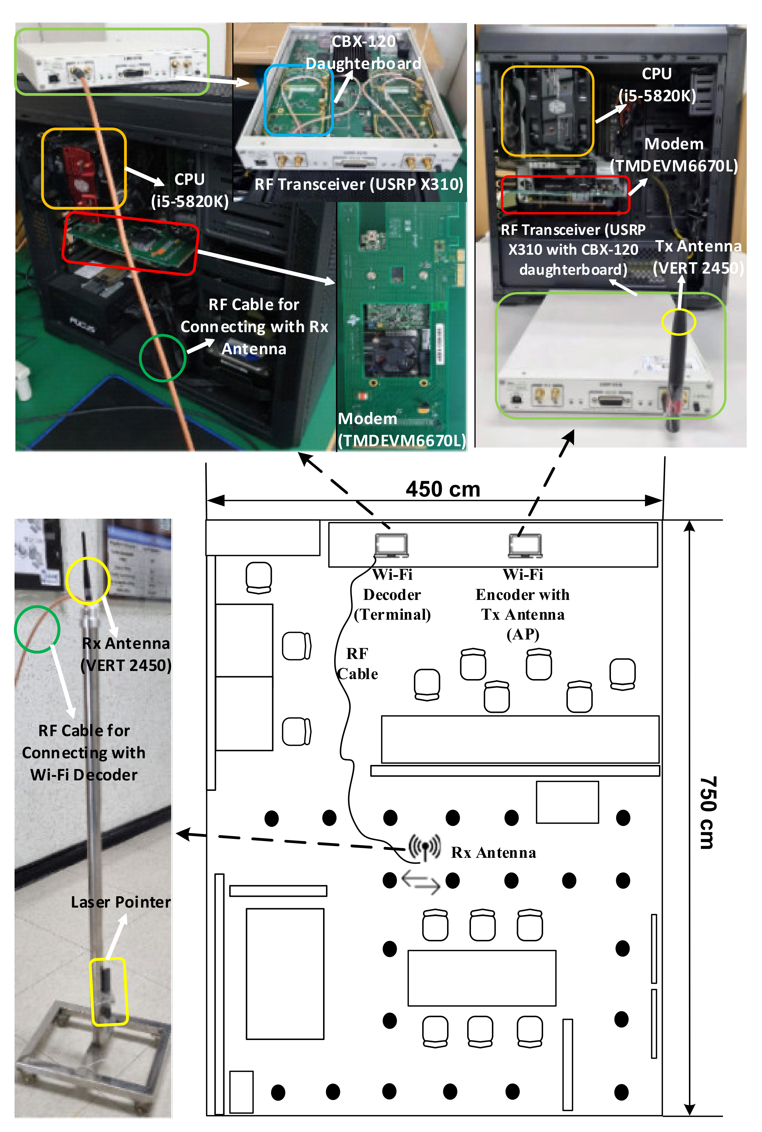
The overall IPS implementation, comprising an encoding AP and decoding MD in an indoor environment, is illustrated in
Figure 10. The implemented AP transmits a Wi-Fi downlink (DL) signal to the MD to receive it. The Tx AP comprises the following four parts: an i5-5820k central processing unit to control the Tx AP; a TMDEVM6670L [
28] modem to encode the Tx Wi-Fi data; a USRP Ettus X310 RF transceiver with CBX-120 daughterboard [
29] for digital-to-analog conversion and frequency up-conversion; and an omnidirectional antenna VERT2450 to radiate the Wi-Fi DL signal, which is denoted in orange, red, green, and yellow colors, respectively. The Rx MD comprises four parts, of which the functionalities are the same as for the Tx AP, except that the MD receives the Wi-Fi signal and the AP transmits the Wi-Fi signal. Note that the Rx antenna connected to the MD via an RF cable was installed on a movable stand such that the CSI could be collected at any desired position; therefore, the movable MD antenna can collect the CSI for any desired trajectory between RPs, 21 of which are denoted as black points in
Figure 10. To track the trajectory as accurately as possible while collecting the CSI, a laser pointer was strapped at the bottom of the movable Rx antenna stand.
6. Experimental Results
The proposed deep learning models of 1DCNN-LSTM and GAN were implemented with TensorFlow 2.0 on an NVidia RTX 2080Ti GPU using the Ubuntu 20.04 operating system. The dataset for training and testing the neural networks was obtained from the proposed IPS—the hardware implementation is detailed in
Section 4.
6.1. Dataset of Trajectory CSI for Experiments
As mentioned in
Section 3, our dataset was obtained from 20 trajectories in five routes, with 21 RPs in total. Each route comprises four trajectories, which brings about the 20 trajectories in total for our experiments. For each trajectory, the trajectory CSI was measured 100 times using the proposed data collection method described in
Section 3. The dimension of the data samples of each trajectory CSI is set to be 2000 × 56 because we have 2000 CSI samples from each of the continuously measured CSI trajectories, with each sample comprising 56 subcarriers, as shown in
Figure 7. Therefore, there are 20 data groups corresponding to 20 trajectories in the dataset. Each data group is labeled with the corresponding trajectories (0~19).
Among the 100 measurements for each trajectory, one out of every five trajectory CSI measurements were selected to build the test dataset, whereas the remaining measurements were the training dataset. Consequently, our dataset comprises 80 measurements of the trajectory CSI for the training dataset and 20 for the test dataset. The 100 measurements for each trajectory must be shuffled well enough such that the training data can be allocated as uniformly as possible over the entire observation period. Consequently, the total number of samples in the training data set is 8,960,000 per trajectory (=80 measurements of 2000 samples for each of 56 subcarriers) while that of the test dataset is 2,240,000 per trajectory (=20 measurements of 2000 samples for each of 56 subcarriers). By using the abovementioned training and test datasets, the proposed deep learning networks are trained and tested to construct the optimal IPS.
6.2. Impact of Convolutional Filter Dimension of 1DCNN
To achieve the best-optimized model for the 1DCNN, we conducted experiments to evaluate the impact of the convolutional filter dimension on the 1DCNN performance based on the number of convolutional layers and filters.
Table 1 shows a comparison of 1DCNN performances based on different numbers of filters and different numbers of layers—one can observe that the accuracy is generally enhanced as the number of layers increases. This is because the learning capability is improved as the number of convolutional layers increases. In addition, as the number of filters increases from 16 to 64, the mean distance error decreases from 1.94 to 1.74 m; however, as the number of filters increases to 128, the mean distance error of the IPS worsens to 2.24 m. This indicates that an excessively large number of filters may result in worse IPS performance because it makes the training of the neural network more difficult.
We also observed the performance of the IPS as a function of the number of convolutional layers with various numbers of convolutional filters employed at each layer. Through extensive experiments, we found that the 256-128-64-32 configuration provides the lowest mean distance error, i.e., 1.34 m, among all the observed configurations. However, the training time for this configuration, i.e., 268 s, was much longer than that for most other configurations because of its four-layered structure with numerous convolutional filters. In the case of both the mean distance error and training time, we found that the configuration of 64-32 provides reasonably good performance with a mean distance error of 1.35 m, which is only 0.75% higher than that of the configuration of 256-128-64-32, and the training time is 134 s, which is approximately 50% faster than that of the configuration of 256-128-64-32.
From the above experiments, we observed that a double-layered model with 64 filters in the first layer and 32 filters in the second layer provided the best performance in terms of both the mean distance error and training time in the indoor experimental environment described in
Section 4. Although a 1DCNN with more than two layers may provide similar or even slightly better mean distance error performance, it inherently leads to a long training time because of the challenge of training the given neural networks. Consequently, a 1DCNN with fewer layers and a small number of filters in each layer might be preferred in terms of the training speed.
Table 2 lists the detailed parameters of the proposed 1DCNN structure.
6.3. Impact of the Number of Segments T
The number of segments
T as described in
Section 5.2 increases when the concatenated trajectory CSI generated by concatenating a set of trajectory CSI in a predetermined route is divided into more segments. As the number of segments
T increases, more 1DCNNs are utilized to extract features from the corresponding segment. To find the optimal
T for the 1DCNN-LSTM architecture, we conducted extensive experimental tests on different values of
T. The detailed parameters for each LSTM of the proposed IPS are listed in
Table 3.
The performance of the IPS based on
T is summarized in
Table 4. It can be observed that the localization mean distance error is enhanced from 1.59 to 1.18 m as
increases from 1 to 4. In our experiments, it was found that the best performance was obtained when
was set to 5, yielding a mean distance error and standard deviation of 0.96 and 0.63 m, respectively. However, as
increases beyond 5, the performance of the IPS degrades, which indicates that numerous segments do not necessarily provide better performance, owing to the accumulated errors at each segment. Therefore, segments
should be sufficiently large to obtain sufficient information from the previous segments. If the value of
is too large, then it is more likely that invalid information can be generated from at least one LSTM, which will result in inaccurate predictions for all the following LSTMs.
6.4. Impact of the Number of Units in LSTM
For each LSTM, the number of units, which is related to the capacity of the LSTM for learning the input data, must be set up with an appropriate value in such a way that it causes neither over-fitting with an excessively large value nor under-fitting with an excessively small value. Thus, the tuning of this hyperparameter is generally determined empirically through experiments.
Figure 14 shows how the number of units in each LSTM results in the training time and loss. The loss of the model during the training period decreases as the number of units employed in LSTM increases. However, when the number of units increases beyond 128, the training time rapidly increases due to numerous parameters being trained, whereas the loss is not decreased conspicuously anymore. For instance, when the number of units is 1024, the training time almost doubles compared to when the number of units is 128, where the loss is almost constant. The trade-off between the training time and loss has led to the conclusion that 128 is the optimal value for the number of units in each LSTM for our model based on our extensive experiments.
6.5. Impact of the Batch Size
The number of samples in the training dataset used to estimate the gradient of the loss before the model weights are updated is denoted as the batch size [
40]. It is an important hyperparameter that should be well tuned to optimize the system’s dynamics, such as the training speed and stability of the learning process.
Figure 15 shows how the batch size impacts the training time and loss. As the batch size increases from 1 to 1024, the time required for training the 1DCNN-LSTM is decreased exponentially. As the batch size increases beyond 32, the training time converges nearly to 100 s. Conversely, the loss of the model decreases from 0.1405 to 0.0261 as the batch size increases from 1 to 64, owing to the increase of the speed for updating the weights of the model; however, as the batch size increases beyond 64 (up to 1024), the loss increases, owing to the poor generalization of the mapping between the input and output of the model. The results of the extensive experiments show that the optimal value for the batch size of our model was 64.
6.6. Impact of the Number of Trajectories
The objective of this subsection is to verify that the route prediction accuracy is improved as we increase the amount of input data of the proposed neural network by concatenating several consecutive trajectory CSI of a given route. With the five routes predetermined, as shown in
Figure 9, the proposed IPS predicts which route among the five predetermined routes the test trajectory/trajectories belong to.
Figure 16 illustrates confusion matrices representing the route prediction accuracy according to the number of trajectories, where
Figure 16a–d represent the results obtained by using the proposed 1DCNN-LSTM, with the number of input trajectories being one, two, three, and four, respectively. It can be easily observed that the probability for the correct route prediction increases as the number of trajectories employed as an input of the proposed IPS increases. It is also noteworthy that all the trajectory CSI that has been already used should not be discarded from the input dataset of the neural network in order to be reused together with the trajectory CSI to be collected later.
6.7. Performance Analysis on GAN
The objective of this subsection is to present the performance of the proposed IPS, which employs the synthetic data provided by the GAN model discussed in
Section 5. More specifically, the performance is analyzed as a function of the portion of synthetic data added to the training dataset described in
Section 6.
To observe how the synthetic data provided by the GAN model enhance the performance of the proposed IPS, we performed two experiments as follows. In the first experiment, 20% (i.e., 16 measurements) of the entire training data was randomly selected and presented to the GAN model to generate a set of synthetic data, which was added to the dataset of the 16 real measurements to increase the total quantity of the training dataset. Subsequently, the performance of the proposed IPS was analyzed as a function of the number of synthetic data added to the 16 real measurements. In the second experiment, we performed the same experiments as the first, except that all the training data (i.e., 80 measurements) were used along with the synthetic data as the training dataset.
Table 5 presents the performance of the proposed IPS in terms of test accuracy and log-likelihood loss based on the number of synthetic data employed together with the actual measurements. The accuracy shown in
Table 5 is defined as (
), where
is the number of true predictions for the test data and
is the total number of trajectories CSI, which is 20 (the total number of trajectories) × 20 (the total number of test samples per trajectory) in our experiments. As
Table 5 shows, the accuracy of the IPS is only 71.2% when the 16 real training measurements were used with no synthetic data for training the neural network. When all 80 real training measurements were used without the synthetic data for training the neural network, the accuracy was 93.3%, which indicates that the IPS performed better when more training data were provided. However, as we added 100 synthetic data generated from the 16 samples using the GAN, the accuracy of the IPS was significantly improved from 71.2% to 93.8%, which is nearly equivalent to the case of the IPS trained with the 80 real measurements. As the amount of synthetic data added to the training dataset increases, the accuracy of the IPS is enhanced and then saturated after adding approximately 300 synthetic data to 20% of the real data, i.e., 16 measurements.
Table 5 shows the accuracy of the IPS when the dataset consists of 20% real data and 80% synthetic data generated using GAN. We also conducted an experiment on the relationship between the classification accuracy and the percentage of real data used for generating synthetic data using GAN; this experiment shows how many real measurements are actually required to generate synthetic training data that can efficiently enhance the IPS performance.
Figure 17 illustrates a comparison of classification accuracy between using real data only and using real data combined with synthetic data. In our experiments, as shown in
Figure 17, the test accuracy increases as the number of real measurements used for generating the synthetic data increases from 4 to 80, which is 5–100% of the 80 real training measurements. The accuracy is only 42% when 5% of the real measurements are used to train the GAN. By adding synthetic data generated with 5% of the real measurements, the accuracy is enhanced to 78%. As the percentage of real data used to generate synthetic data increased from 5% to 25%, the accuracy of the IPS is enhanced from 78% to 96.3%, which is significantly higher than that of the IPS trained only with the real data. It can also be observed that more than 35% of real data (28 samples) being used by the GAN does not conspicuously enhance the accuracy, meaning the GAN employed in the proposed IPS can provide enough valid synthetic data with only 35% of the real trajectory CSI.
6.8. Performance Comparison with State-of-the-Art Methods
State-of-the-art neural networks, i.e., ConFi [
21], DeepFi [
16], and Horus [
41], were used to compare with the proposed neural networks, i.e., 1DCNN-LSTM aided by the GAN, to evaluate the performance of the proposed IPS. The optimized configurations obtained from our extensive experiments were used for 1DCNN-LSTM. To be more specific, there were two convolutional layers with 64 filters in the first layer and 32 filters in the second layer for each 1DCNN, the number of units in each LSTM was 128, and there were five segments.
Table 6 shows the numerical results obtained by the proposed method and other state-of-the-art methods. The best performance is observed from the proposed 1DCNN-LSTM model with the mean distance error being 0.74 m, outperforming the ConFi, DeepFi, and Horus methods by 46.0%, 47.9%, and 61.9%, respectively.
Figure 18 shows the cumulative distribution function for all four methods—we see that the proposed 1DCNN-LSTM outperforms ConFi, DeepFi, and Horus with a distance error probability of 87% within 1 m, 95% within 2 m, and 100% within 3 m.
6.9. Performance Comparison with Different Spacing between RPs in Two Different Signal Environments
The objective of this subsection is to present the performance of the proposed IPS with a few different selections for the spacing between RPs in two different signal environments. The two different indoor signal environments are (1) narrow laboratory with various furniture, and (2) relatively wide corridor, of which the photos are shown in
Figure 19a,b, respectively.
Table 7 shows the numerical results obtained from experimental tests using the proposed method in the abovementioned two different indoor signal environments with four different values for the spacing, 60 cm, 80 cm, 100 cm, and 120 cm. First of all, it has been observed that the performances in the two different signal environments are quite different from each other. The performance obtained in the wide corridor is much better than that of the narrow laboratory. The main reason is that the Wi-Fi signal in the narrow laboratory suffers more severely than that of the wide corridor from adverse multipath effects. The lowest mean error is 0.73 m with the spacing being 60 cm in the laboratory signal environment, whereas the lowest mean error is 0.43 m with the spacing being 100 cm in the corridor signal environment. Second of all, it has been observed that, for both laboratory and corridor signal environments, the value for the inter-RP spacing turns out to be not a major factor affecting the performance of the proposed IPS, which should be taken as granted because our method is based on the trajectory CSI continuously measured in between adjacent RPs instead of the single-point CSI measured at each RP. It means that the proposed IPS exploits all the CSI values between RPs, which in other words indicates that the effective value for the spacing in the proposed IPS is nearly 0.


