Relationships among them are nonlinear and the modeled signal is discrete, which can be defined as:
where
,
and
are the system output, input, and noise sequences, respectively;
,
, and
are the maximum lags for the system output, input and noise;
is some unknown nonlinear function,
d is a time delay typically set to
.
The problem of this approach is that the developer has to suggest possible types of nonlinearity because the number of nonlinearities is quite high. These can be:
For this reason, modeling a nonlinear system brings the possibility of unknowingly making a fatal error. If the system under test has a nonlinearity that is not assumed, the model will not be fitted the data. In NARMAX methods, the only limit is the assumption made by the modeler. Here, some nonlinear modeling systems are presented.
2.3.1. OLS
This work proposes using the Orthogonal Least Squares (OLS) algorithm to establish the correspondence between the face features based on the camera and the coordinates projected by the gaze on the screen. This approach has been used on nonlinear systems because OLS will search through all possible candidate models to select the better approach.
The main idea of the OLS estimator is to introduce an auxiliary model whose elements are orthogonal to the signal that is modeled, as in the Wiener Series. Then, subsequent parts of the orthogonal model can be determined in turn, and then the parameters of the searched model can be calculated based on them. Iterative repetition of the steps of this method allows not only finding unbiased model estimators, but also showing what contribution each of them has in the final modeling result.
Considerations should begin with the assumption of the general model:
where
is the modeled system response for
;
are the model parameters
associated to the regressors
and
is the external noise or error at the moment
.
Regressors
are defined as the combination of delayed signal values or delayed external signals. In the general case, the function of the delayed members of the model can take any non-linear form. For the model, it is also assumed that each regressor
is independent of the model parameters
, therefore:
The goal of the estimator is to transform the model specified in Equation (
2) into an auxiliary model whose elements are orthogonal to each other. This type of model has the form:
where
are the parameters of the orthogonal model and
(
) are the orthogonal components of the model. The orthogonality condition is then presented as:
The orthogonalization procedure for the model from Equation (
2) can be summarized as:
where parameter
associates the components of the output model from Equation (
3) with the orthogonal model according to the following form:
This allows, based on previously established regressors, to develop a model based on orthogonal components, and to recreate the basic model from this type of model.
2.3.2. ERR
The problem in carrying out OLS estimation is the criterion for selecting subsequent regressors for the orthogonal model being created. Remembering that the model also has noise
e, the energy (or variance) of the system can be represented as:
where
y is the modeled signal vector,
are the coefficients standing next to elements of the orthogonal model,
are the vector elements of the orthogonal model,
e is the vector of noise samples and
N is the number of signal samples. It can be stated that:
where
is the Error Reduction Ratio and
is the Error to Signal Ratio. To measure the significance of each model parameter, the Error Reduction Ratio (ERR) is used, which indicates the system improvement, in percentage (0–1). It can be accounted by including the model parameters. This capability is important for the model to get the best model, without getting a complex one. ERR allows the model to get only the best parameters in order to achieve best model performance without a high training time and without complex the model.
When the sum of subsequent values ERR tends to one means the modeling process can stop (). Comparison of individual values for various elements of the model shows which of them are the most influenced on the signal of the designated model.
2.3.3. FROLS
Using the OLS estimator and coefficient ERR describes the FROLS (Forward Regression with Orthogonal Least Squares) nonlinear modeling algorithm, a forward regression algorithm using the orthogonal sum of the least squares. It is assumed that the selection of subsequent regressors for the OLS estimator should be conditioned by the highest value ERR for a given regressor. This allows choosing the model member that reduces the modeling error to the greatest extent and to stop modeling when ESR will have a satisfactory value. In the following sections, steps in modeling according to the FROLS algorithm will be presented.
Step 1. Data Collection
In order to perform modeling, acquisition of the test signal waveforms is required,
(X_pixel, Y_pixel), as well as external input signals,
(OpenFace parameters), which affect the system under study. The signal should be collected as discrete or transformed into such a form. In addition, the recorded waveform should have as little external noise as possible and should not be subjected to filtration, which may disturb the identification process. According to the author of the method [
35], if the noise presents in the signal is zero-mean white noise, it does not affect the ERR value and the identification process.
Step 2. Defining the Modelling Framework
Because the number of possible nonlinearities is very high, a priori assumption is required to define the search method. These requirements can be formulated answering the following questions:
What is the maximum delay of the AR term ()? (Output signal)?
What is the maximum delay of external signals ()? (Input signal)?
What nonlinearities are predicted and what is their maximum degree (l)?
After the developer has provided the answer to these questions, the following parts of the model are known: , , …, , , , …, . Where y is the signal under test, is one of the external input signals, is the maximum delay of the signal under test and is the maximum delay of one of the external input signals. The non-linearity that binds these members is also known, which allows the next step to be taken. In the case where the non-linearity is a polynomial, the maximum degree of non-linearity determines the maximum power occurring in this polynomial.
Step 3. Determination of the Regressor Vector
Knowing the modeling framework defined in the previous step, we must determine a vector containing all possible regressors for a given signal. For example, a system with one output (
y) and one input (
u) with
, where nonlinearity is modeled as a polynomial up to the second degree,
. Then, the regressor vector will consist of a combination of signals:
,
,
,
according to the maximum polynomial degree. Including the constant component marked as
, regressor vector marked as
D, will be defined as:
Step 4. Choosing the First Element
Once the regressor vector has been specified, the database of the created model is known. Choosing the first one requires determining the value of ERR for each element of the vector
, where
m is the number of potential regressors.
where
corresponds to the highest regressor and it is accepted as the first element of the orthogonal model. The parameters
g and
are saved.
After saving the found regressor and its associated values, the search is restarted to find the next member of the orthogonal model.
Step 5. Selecting the Next Elements of the Model
The next steps are analogously performed to the first step, with the difference that the orthogonal model already has a certain number of terms, depending on the number of steps previously performed. Calculation of
values for potential new members of the model must be made again, in relation to the current form of the model. Therefore, the regressor index is searched (marked as
) about the highest
for the current model form, where
s) is the current step. The regressor vector is marked as
and does not contain the members selected in the previous steps. Then, for
and
, we have:
After finding
, which corresponds to the highest regressor
, the orthogonal model is extended by another member,
, along with the corresponding parameter
. The
value for the selected element is saved, and from the vector
D the selected regressor is deleted. In addition, parameter values
are determined according to the following equations:
This step is repeated until the
ESR value is satisfactory:
where
is the number of selected regressors. A certain limit is necessary for
ESR, which will decide the end of the modeling.
2.3.5. Determination of the Final Model
When
regressors are selected, it is necessary to determinate their parameters. Assuming a low value of
, the general and ortogonalized models are equal to:
In the above equation, the only unknowns are
, because regressors
were selected during modeling, and the elements of the orthogonal model
along with their parameters were appointed on an ongoing basis during the process. Therefore, it is necessary to perform the conversion from the orthogonal model to the initial model by performing an inverse process to the previous orthogonalization. Knowing the values of the elements
for
, the following matrix is specified:
which can be included in equation:
where
and
. Solving this equation, model parameters are obtained, thus determining the full output model.
The output has a vector form of two coordinates (X_pixel, Y_pixel), so, two models have to be calculated in order to obtain the system output as required.
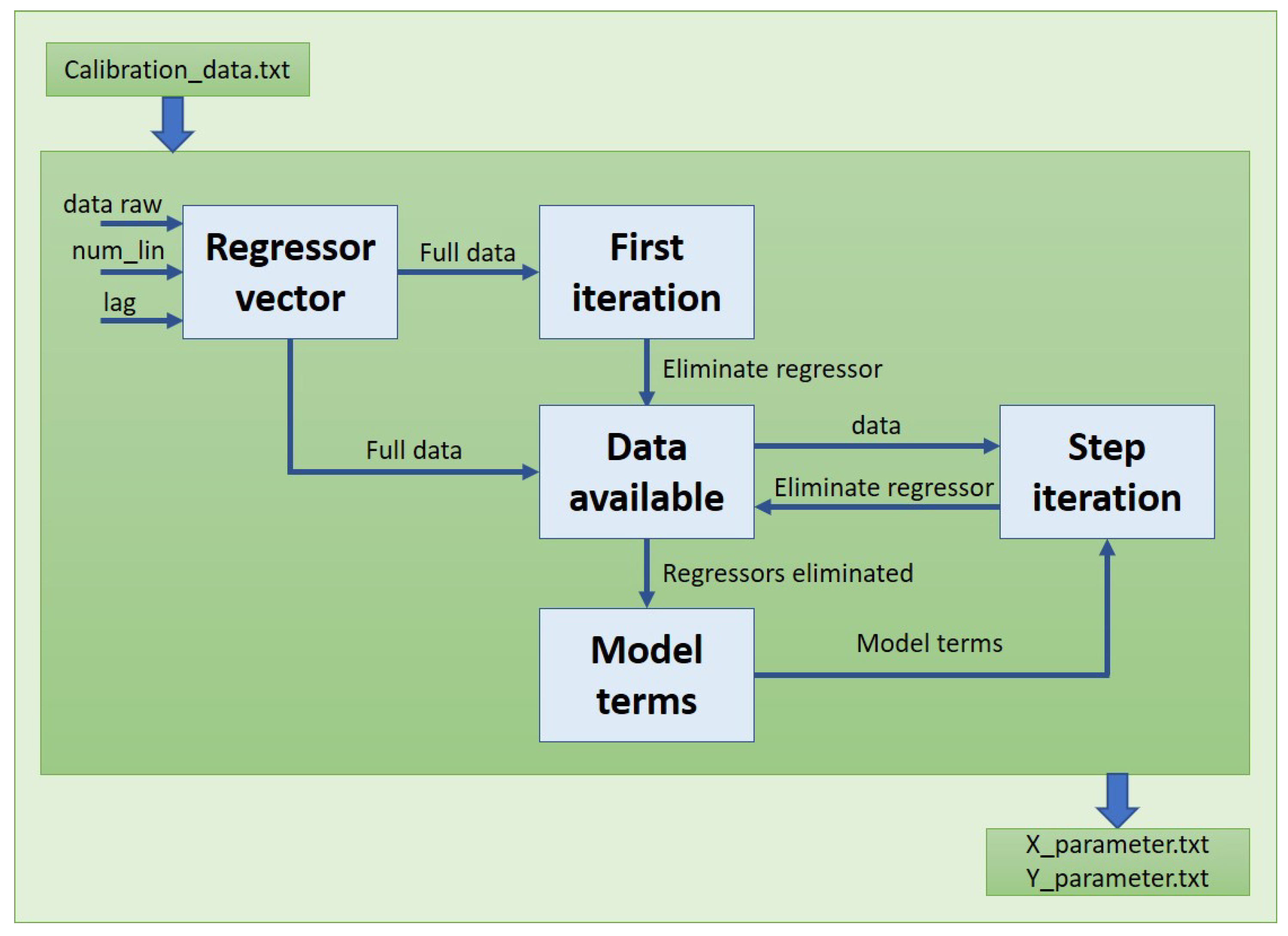
Three main parts compose the framework used on this calibration step, and how the subsystems are communicated among them in order to achieve the best result. The first one is in charge of getting data to calibrate. The second one calculates the regressors for the model. Furthermore, finally, the last one uses these regressors and sends the topic to the ROS environment.
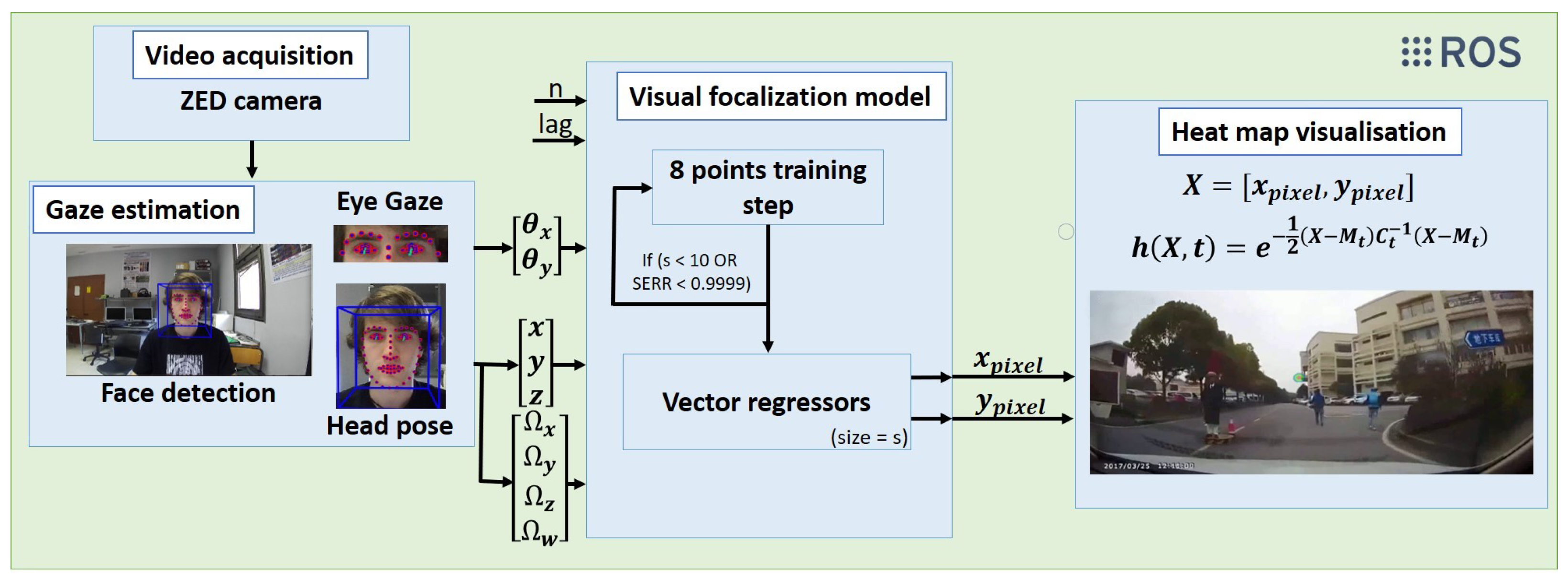
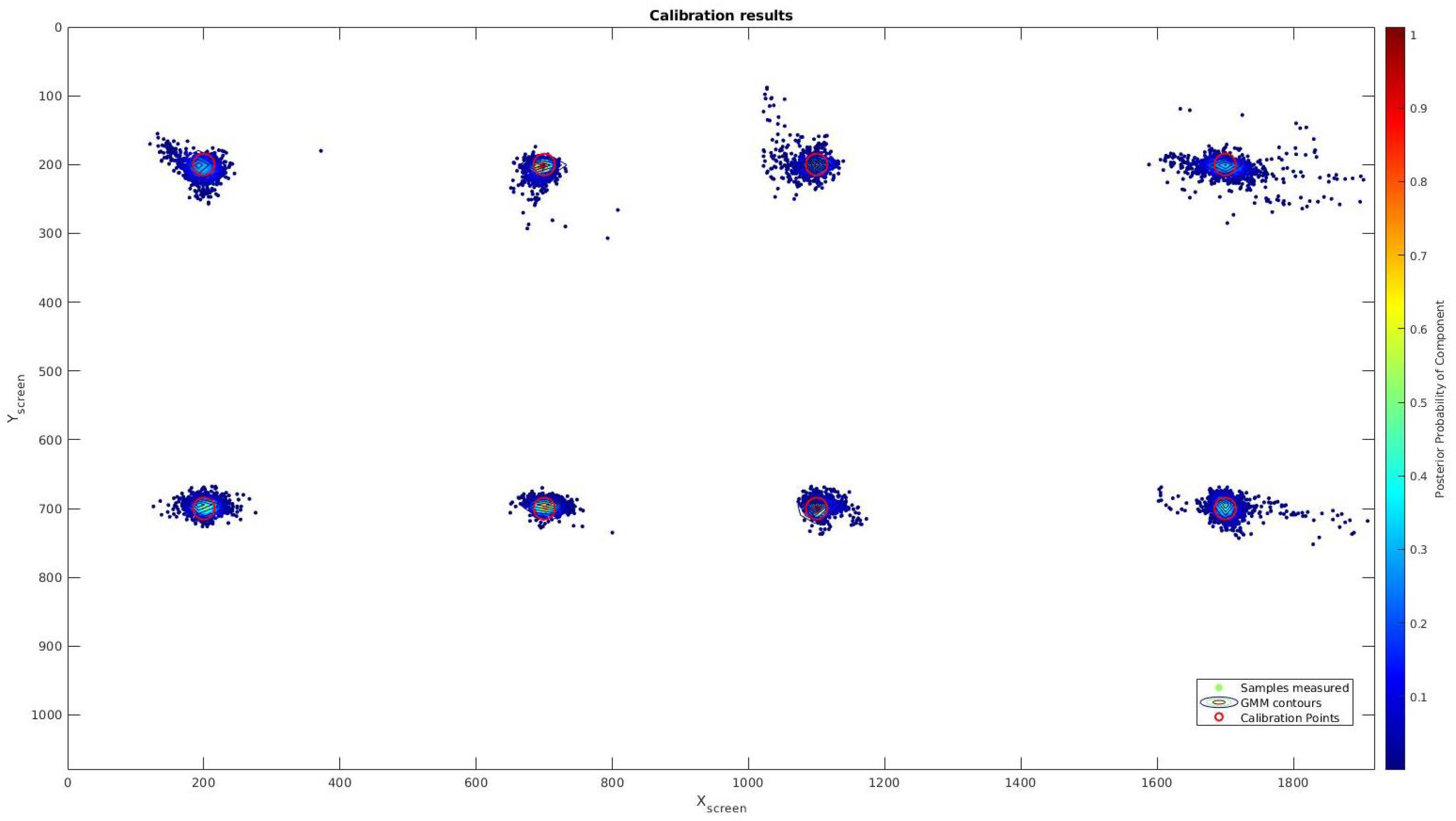
In order to achieve this calibration method, a training method is necessary. So, at the beginning of any test, the user has to look at eight points around the screen. Points are displayed during 8 s, but in order to get a better accuracy on the model, the first two seconds are removed because in this time the eyes are in transition between fixations.
To perform this task, the eight points are displayed in red over a white image using OpenCV. These points have a 30 pixel radio and are placed on the following positions in pixels: , , , , , , and . After training, these points will be evaluated during a testing procedure.
Data are composed of the point where the user is looking at (X_pixel, Y_pixel) and the data provided by OpenFace for the gaze and the head for this position, which is formed by:
Gaze angle X ();
Gaze angle Y ();
Head position X (x);
Head position Y (y);
Head position Z (z);
Head rotation X ();
Head rotation Y ();
Head rotation Z ();
Head rotation W ().
Data are referenced to the camera and saved on a
.txt file with the next structure: Gaze angle
X; Gaze angle
Y; Head position
X; Head position
Y; Head position
Z; Head rotation
X; Head rotation
Y; Head rotation
Z; Head rotation
W;
X_pixel; and
Y_pixel. These are the parameters chosen, because gaze focalization systems take as input: eyeball orientation and head pose (orientation and position of the head) [
16]. Instead of eyeball orientation, we use a gaze vector provided by OpenFace 2.0 to obtain a more accurate gaze focalization system.
The file created with the data recorded for each test will be charged on the next step of the model where a training procedure is carried out to calculate the parameters, as it is defined on
Figure 3, where the data feed the model and following the steps described earlier to obtain the regressors and their parameters for the two models.
NARMAX model is fit with these parameters. The model will use the parameters necessary to fit the model to the output as best as possible. After some experiments, the best option is obtained for a Sum Error Reduction Ratio (SERR) higher than 0.9999 or 10 regressors. More regressors complicate the model with a slight improvement on accuracy and over-fit the model.


 ,
, 


