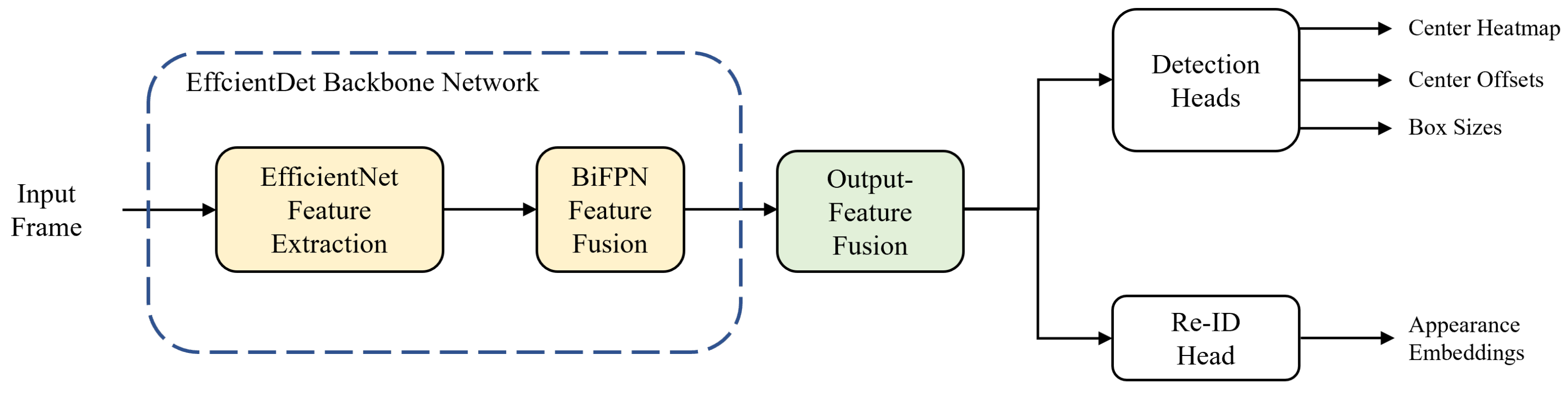
The overall flowchart of our single-shot MOT system is shown in
Figure 1. The MOT system begins by forward-passing an input frame into the backbone network. We use EfficientDet [
41] as a backbone network; it consists of two stages: feature extraction and fusion. In the first stage, EfficientNet [
42] performs feature extraction and produces three multi-scale feature maps. In the second stage, the features go through the process of feature fusion via the bi-directional feature pyramid network (BiFPN) [
41] layers and five multi-scale feature maps are taken out from the backbone network. Before being transferred to prediction heads, the output features are fused into one to match the feature dimensions. In
Section 3.1 and
Section 3.2, we describe the backbone network and output-feature fusion of the proposed method, respectively. For predictions of the center heatmap, center offsets, and box sizes of the objects, the integrated feature is transferred to the detection head. Likewise, the same procedure is carried out for the re-ID head to extract appearance embeddings from the feature map. Finally, online association is applied to the output results from the prediction heads to match the IDs of objects in the current and previous frames.
3.1. Backbone Network Architecture
A backbone network plays a significant role in the overall MOT system, in that it generates features that are essential for further steps. The performance of a MOT system varies greatly, depending on how the backbone network extracts and aggregates high-quality features with its own method. In our proposed method, we adopt EfficientDet [
41] as a backbone network to improve the performance of MOT by increasing the accuracy while minimizing the loss of efficiency. We present two reasons for using EfficientDet. EfficientNet [
42], which is the backbone network of EfficientDet, shows outstanding performance for a small number of parameters, and achieves high accuracy and a fast inference speed. The second reason is that BiFPN [
41], which is the fusion network, increases the average precision (AP) whilst having a lower computational cost, as compared to others [
43,
44].
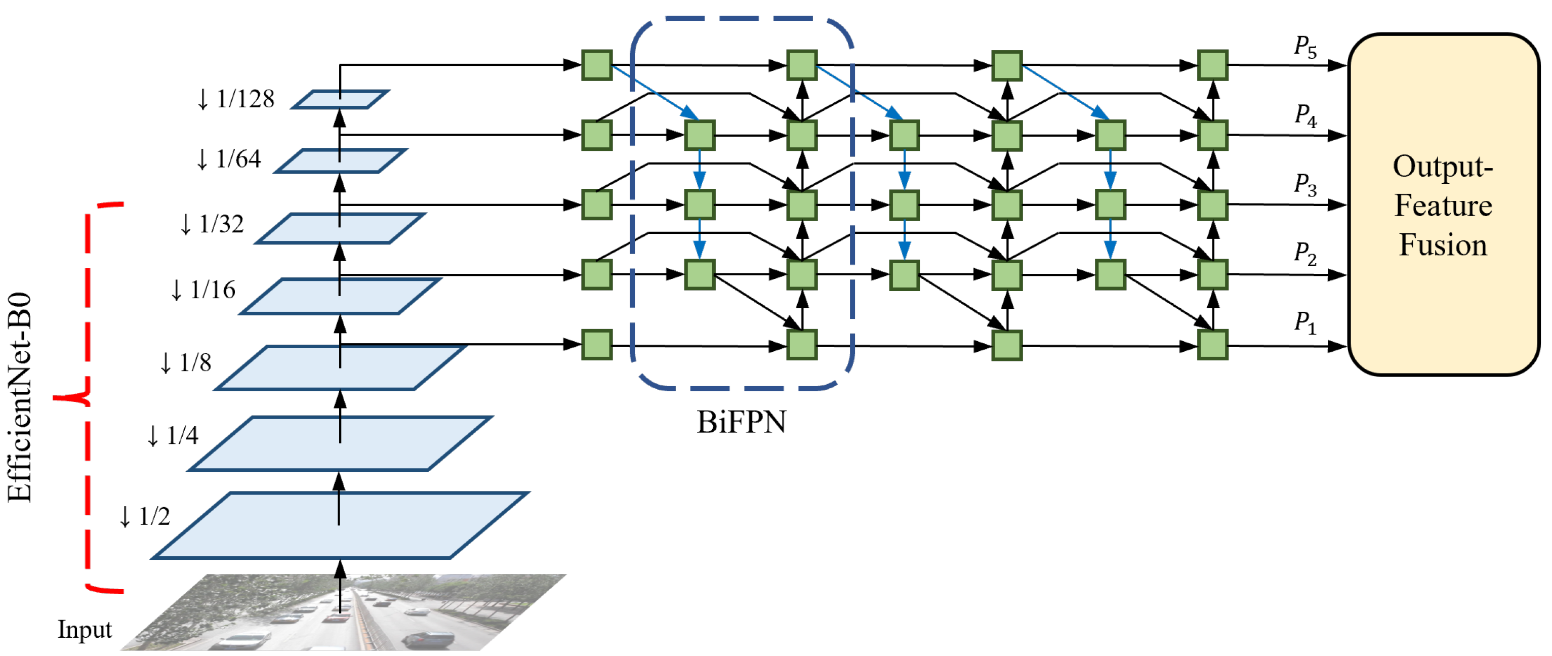
EfficientDet offers eight different optimized models based on thorough observations by considering depth (number of layers), width (number of channels), and input resolution. Among them, we utilize EfficientDet-D0, which is the most lightweight model that repeats the BiFPN layers three times, uses 64 channels, and takes an input resolution of 512 × 512. EfficientDet-D0 is selected to minimize the decrease in the inference speed. This is because scaling up the three factors reduces the efficiency to the extent where it differs significantly from the baseline [
5]. The backbone network architecture of the proposed method is shown in
Figure 2. An input frame is first forward-passed into the backbone network, and EfficientNet produces three multi-scale features with resolutions of 8, 16, and 32 times lower than the input size, respectively. In this process, EfficientNet effectively decreases the parameters and FLOPs by using the mobile inverted bottleneck convolution (MBConv) [
45,
46]. As a pair, EfficientNet-B0 is applied to the feature extractor. The original EfficientNet-B0 operates 18 convolutions of different kernel sizes, including two standard convolutions and 16 MBConvs, and uses a fully-connected layer for classification. However, because EfficientNet-B0 only performs feature extraction without additional processes of classification in EfficientDet-D0, the last 1 × 1 convolutional layer and the following fully-connected layer are removed from the original model. The structure and specifications of the modified EfficientNet-B0 are listed in
Table 1.
The following step details how to fuse the multi-scale features with BiFPN. Before sending the three multi-scale features to the BiFPN layers, a 1 × 1 convolution is performed on each feature map to set the number of channels to 64 and two additional lower-resolution features are extracted by max pooling. Therefore, a total of five multi-scale features, with the same number of channels, are transferred to the BiFPN layers. BiFPN effectively fuses features by applying several techniques to PANet [
47], which utilizes both top-down and bottom-up pathways. The modifications for optimization are as follows: (1) Cut off nodes that have negligible influence on the quality of feature maps. (2) Add extra skip connections. (3) Repeat the entire BiFPN layer multiple times. By leveraging the optimized network, the output features {
} of the backbone network become highly robust to scale variations.
Input resolution greatly affects the development of a CNN. In particular, it becomes significantly important in tasks that require rich representations of features for small objects, such as object detection and MOT. In general, a larger input resolution is accompanied by a larger network size and results in higher accuracy. However, the increase in both factors critically harms the inference speed by drastically increasing the computations. Therefore, it is necessary to scrutinize the performance of the CNN with different input sizes and different numbers of network parameters to find the optimal combination that optimizes the balance between accuracy and efficiency. In Tan et al. [
41], EfficientDet-D0 is designed to operate with an input resolution of 512 × 512. In our method, we intentionally set an input size of 1024 × 512 (width × height). This idea is based on the observation that simply increasing the input resolution of a lightweight network benefits the efficiency more than using a heavyweight network of large resolution, while both show similar performances for the accuracy. An aspect ratio of the input is also significant for the performance of the CNN. This is because a wide discrepancy in the aspect ratio between the input and frame leads to a heavy loss of information when the frame is resized. Considering the frame size of videos in real-world applications, the aspect ratio is set to 2:1 in our proposed method. The input resolution of the feature maps for each operation is shown in
Table 1.
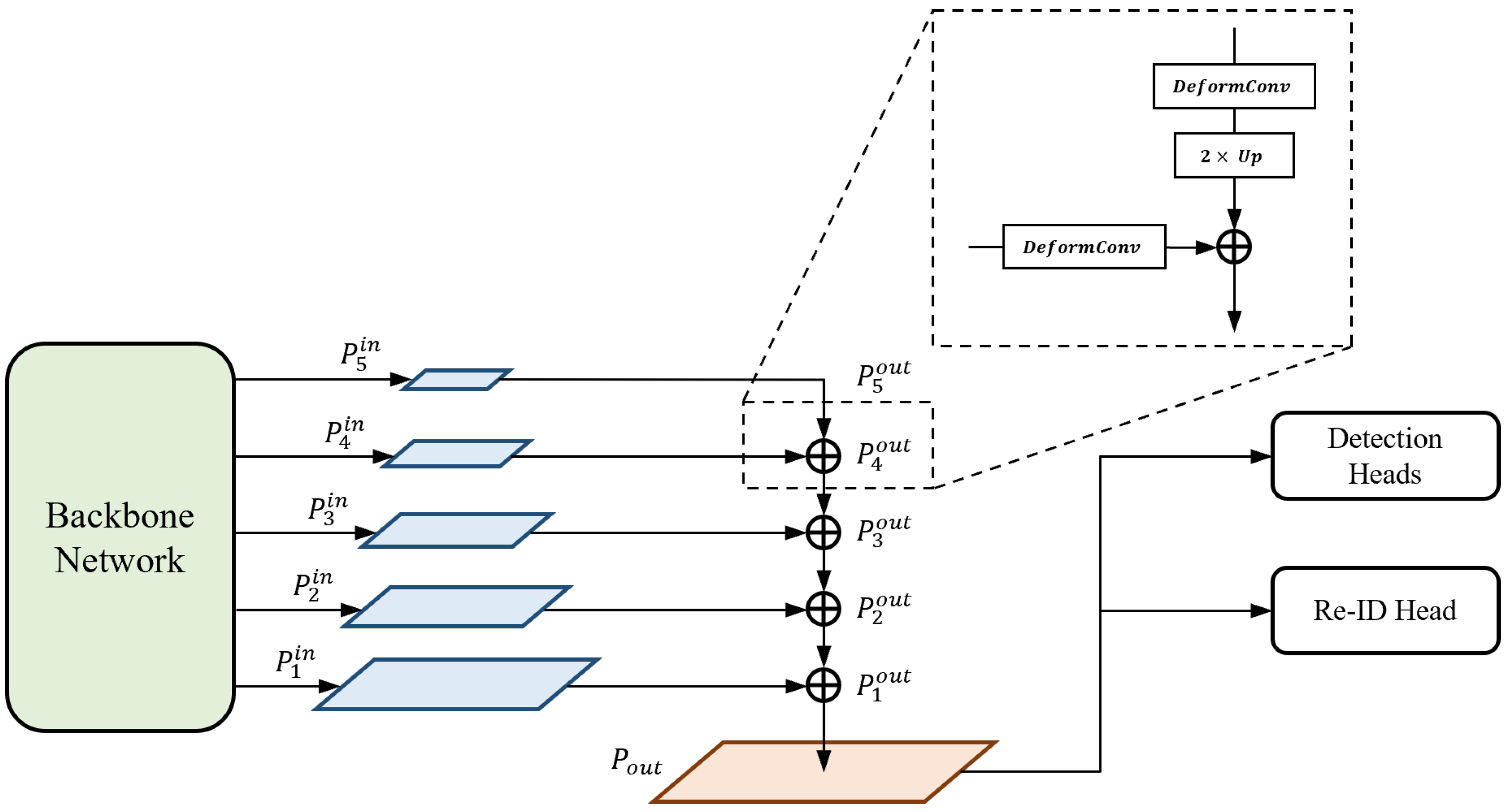
3.2. Output-Feature Fusion
Output-feature fusion is a vital process for integrating multi-scale features output from a backbone network into a single feature map for subsequent operations. Based on previous studies that utilize heatmaps for predictions [
48,
49,
50,
51], our single-shot MOT system performs object detection and embedding extraction on a single high-resolution feature map. Therefore, it is crucially important for our network to generate a single feature that potentially comprises rich representations.
The output-feature fusion network architecture of the proposed method is illustrated in
Figure 3. We append the structure of the feature pyramid network (FPN) [
43] to the end of the backbone network for fusion. FPN serially merges multi-scale features from high to low levels to produce semantically strong feature maps. The features from the top-down pathway and lateral connections are fused using Equation (
1):
where {
} are the multi-scale input features transferred from the backbone network, {
} are the output features,
is the deformable convolutional operation, and
is the up-scaling operation. At each level, a deformable convolution [
52] is first performed on both features, which are from the higher level and lateral connection, respectively. Inspired by [
5], we use the deformable convolution for every branch in order to adaptively decide the receptive field by applying a learnable offset, which varies depending on the scales of an object, to the grid point of kernels. Subsequently, a lower-resolution feature is up-scaled by a factor of two by the transposed convolution; thus, it is resized to the same resolution as the other. We adopt the concept of the depth-wise convolution [
53] here to reduce the number of parameters and computations. Finally, the feature maps of the same spatial size are fused by element-wise summation and the output is sent to the lower level in order to repeat the entire fusion block.
To generate a final high-resolution feature map that is transferred to prediction heads, we up-scale the feature
of the highest resolution among the feature maps from FPN. The up-scaling process is identical to the combination of the operations
and
, which are used in the top-down pathway of FPN. That is, the feature
is up-scaled by Equation (
2):
where
is the final high-resolution feature map. As a result, given an input image
, where
H and
W are the height and width, respectively, the output-feature fusion network outputs the single high-resolution feature map
, which is utilized for subsequent predictions.
3.3. Prediction Heads
A prediction head is a significant component in the single-shot MOT system because it determines the specific tasks that the system will perform. In general, prediction heads are appended to the end of a backbone network and receive the extracted features needed to carry out various tasks, such as localization and classification of bounding boxes. In our proposed method, the prediction heads are attached to the end of the output-feature fusion network and take the input of a single high-resolution feature map, whose resolution is four times lower than the size of an input image. Based on a feature with rich representations, we utilize three prediction heads for object detection and one re-ID head for embedding extraction. Here, the three prediction heads for object detection are composed of center-heatmap, center-offset, and box-size heads proposed in CenterNet [
50].
In front of each prediction head, a 3 × 3 convolution with 256 channels and a 1 × 1 convolution are performed to make the feature map applicable to the assigned tasks. Specifically, the target of the center-heatmap head has only 1 channel of the heatmap because our single-shot MOT system works for a single class. In the center-offset head, the number of target channels is set to two (for horizontal and vertical offsets), while that in the box-size head is set to four (for top, left, bottom, and right edges of a box). The re-ID head utilizes a target that has 128 channels, which comprise an appearance embedding extracted from an object center.
The center-heatmap head is used to predict the locations of the centers of the objects and aims to estimate the probability of containing the object center at each location of the target heatmap
. The probability is ideally one at the object center and rapidly decreases as the distance between the predicted location and object center increases. In the training stage, the ground-truth heatmap
is set to a 2D Gaussian mixture, where each Gaussian distribution corresponds to a single object. Given a ground-truth object center
in an input image
I, the location is first converted into the down-scaled object center
, and then the 2D Gaussian distribution
is produced by Equation (
3):
where
is the standard deviation, which varies depending on the size of an object. To generate the final ground-truth heatmap
Y, all Gaussian distributions are merged by element-wise maximum, as shown in Equation (
4):
where
N is the number of objects in the input image. We denote the loss function
is the focal loss [
25] for penalty-reduced pixel-wise logistic regression [
49], as shown in Equation (
5):
where
and
are the hyperparameters of the modulating factors in the focal loss. In our proposed method, we set
and
, adopting the values used in CornerNet [
49].
The center-offset head is employed to restore the information of accurate object locations that are lost because of the down-scaling process. The objective of this prediction head is to precisely adjust the positions of objects by applying offsets, which are horizontal and vertical shifts, to the down-scaled object centers. From the target offsets
, we first sample the offsets
only at the down-scaled object center
. Subsequently, the Manhattan distance between the sampled offsets and the ground-truth offsets, which are pre-determined by
, is computed for regression. We denote the loss function
is the L1 loss, as defined by Equation (
6):
The box-size head is utilized for predicting the object sizes by estimating the top, left, bottom, and right edges of the bounding boxes. In our proposed method, the regression of the four edges is used instead of the regression of the height and width for more accurate localization. The training process of the box-size head is similar to that of the center-offset head. Given a ground-truth bounding box
, where
and
are the height and width, respectively, the ground-truth size is computed as
. Afterward, we compute the Manhattan distance between the ground-truth size and the sampled size
from the target size
for the regression. We denote the loss function
is the L1 loss, as shown in Equation (
7):
The re-ID head is used to encode the appearance information of objects, such as shape, color, and view, into the appearance embedding vectors for object re-identification. This head aims to make the embedding vectors of the same-ID objects close to each other and those of the different-ID objects far from each other. In the training stage, we consider all object IDs in the training set as classes. We also append a fully-connected layer that has the same number of output channels of the classes to the re-ID head in order to treat the task as a classification task. From the target of the appearance embedding
, the embedding vector
is first extracted from the down-scaled object center
. Afterward, the class-probability vector
, where
M is the number of object IDs in the training set, is generated by the dense layer and softmax operation. Subsequently, the cross entropy between the class-probability vector and the ground-truth one-hot encoded vector
is computed for regression. We denote the loss function
is the cross-entropy loss, as defined by Equation (
8):
It is necessary to train multiple prediction heads to optimize our overall single-shot MOT system; thus, we approach this work as a multi-task learning problem. Specifically, the automatic balancing of multiple losses using uncertainty [
54] is applied to the multi-task learning of object detection and re-identification. We first define the loss function of detection
by the weighted summation of losses, as shown in Equation (
9):
where
and
are the loss-weight constants. We set
and
, adopting the values used in CenterNet [
50]. Finally, the total loss function
is calculated from Equation (
10):
where
and
are the learnable loss weights of the automatic multi-loss balancing.
3.4. Online Association
Online association is a crucial process in MOT because the detected objects are interpreted as tracklets by the online association algorithm. The association algorithm aims to accurately track objects by maximizing the leverage of the appearance embeddings, with aid from the predicted object locations. The visualization of online association is shown in
Figure 4. In the first frame of a sequence, tracklets are initially activated by the detected objects. Subsequently, we associate the activated tracklets with the newly detected objects in the next frame based on the cosine distances between the embedding vectors. The costs are computed for every combination of the tracklets and objects, whose confidence score is higher than a threshold; the pairs are subsequently matched by the Hungarian algorithm [
27]. Furthermore, we compute the squared Mahalanobis distances between the object centers and state distributions, which are predicted by the Kalman filter [
26], to avoid matching the distant different-ID objects with similar appearances.
For efficient tracklet management, we utilize a tracklet pool, which is a set of categorized tracklets. Here, all tracklets in the pool are categorized into three states: tracked, lost, and removed. In the matching process, if the tracked and lost tracklets from the previous frame are successfully matched with the detected objects in the current frame, the tracked objects remain tracked and the lost objects are re-tracked until subsequent association. However, if there are unmatched tracklets or objects, we mark the unmatched tracklets as lost, while new tracklets are activated for the unmatched objects. Finally, we mark the tracklets as removed if they are lost right after the activation or have been lost for 30 frames in a row.


