1. Introduction
The detection of clouds with airborne instruments is critical when studying the meteorology and climate of the Earth. However, there are other applications where auxiliary systems for cloud detection and characterization are needed, which is the case that concerns us.
Thermography is one of the main techniques for measuring the temperature of things remotely. It is based on InfraRed (IR) cameras to characterize the relationship between the object temperature and the IR energy it emits. Although the first applications of IR cameras were military (World War II), their use spread to many fields since the 1960s. However, the direct application of IR cameras to some applications did not obtain the expected results. Frequently, the lack of knowledge of the physical phenomena involved in the emission, propagation, and measurement of IR radiation led to inappropriate use of commercial IR cameras or prevented a correct interpretation of the images.
To solve a new technological or environmental problem, it is necessary to follow an adequate procedure. The method should begin with a radiometric and spectral characterization of the problem. Afterward, the IR instruments can be developed or adapted according to the previous characterization. Finally, to solve the specific problem, it is necessary to develop specific algorithms that retrieve the physical information from the data provided by the IR instrument: combustion measurements [
1,
2] forest fires, [
3,
4] non-destructive analysis, medical applications [
5], etc.
Nowadays, technology has evolved significantly, and there are extremely high- performance hyperspectral IR systems. Many of these systems are embedded in satellites and can provide very precise information on many phenomena globally.
However, the most current trend in the space sector is moving towards developing small satellites, nanosatellites, or CubeSats. At present, many environmental and technological problems do not require the high spectral resolution that current technology offers. However, they do require simple systems with low cost, low mass, and low energy consumption. In this framework, it makes sense to recover bi-spectral thermography systems, which are simpler and cheaper than sophisticated multispectral systems. The spectral and radiometric characterization of the problem should be the basis to simplify the devices. This alternative approach facilitates observation at higher spatial and temporal resolution and addresses monitoring problems in specific areas. This is also the case of some instruments using ancillary devices to provide complementary but essential information.
Precisely, the work that we present here aims to develop and validate an algorithm to detect clouds from the information provided by a simple bi-spectral IR camera. In the Joint Experiments Missions- Extreme Universe Space Observatory (JEM-EUSO), a secondary instrument (a bi-spectral camera) will carry out the detection of the clouds. However, the relevance of the results we present here goes beyond the JEM-EUSO missions. New instruments for mini and nanosatellite constellations, mainly focused on communications and Earth observation, could use this algorithm.
The objective of the international JEM-EUSO program is to observe Ultra High-Energy Cosmic Rays (UHECRs) to explain the origin and nature of such particles [
6]. When a UHECR collides with an atmospheric nucleus, it causes an Extensive Air Shower (EAS), which is a cascade of charged particles throughout the atmosphere. The charged particles excite nitrogen molecules and we can detect the ultraviolet (UV) radiation produced in this process (fluorescence and Cherenkov radiation). The analysis of the UV images will give information on the UHECR properties. That is the observational principle of all the experiments of the JEM-EUSO program. However, the flux of these particles is extremely low (a few per km
per century at extreme energies such as
E > 5 × 10
eV). The JEM-EUSO Collaboration has addressed that challenge with space observatories. The final objective of the JEM-EUSO program is to realize a space mission with a super-wide-field telescope. It will look down from space onto the night sky to detect UV photons emitted from the EAS generated by UHECRs in the atmosphere. This is also the measuring principle of other pathfinders boarded on balloons and satellites to test the technologies involved in this ambitious program [
7,
8].
However, the presence of clouds between the EAS and the UV telescope may interfere with the EAS measurement. It may also lead to a misinterpretation of the observations. Then, for this type of application, an auxiliary instrument that maps the state of the clouds when a UHECR occurs is essential.
Today there are many weather satellites with instruments capable of determining the state of the sky with great accuracy [
9,
10,
11]. Most of them base their operation on a massive study of bands that allow an exhaustive atmosphere characterization, e.g., MODIS includes 36 spectral bands ranging from
to
m. The Advanced Very High-Resolution Radiometer (AVHRR) is a multispectral sensor with six spectral bands included in NOAA satellites since the last 1970s [
12]. Even the Imaging Infrared Radiometer (IIR), which is part of the payload of the Cloud-Aerosol Lidar and IR Pathfinder Satellite Observation (CALIPSO-NASA), provides information in three spectral bands [
13]. The Spinning Enhance Visible and Infrared Imager (SEVIRI) in MSG (Meteosat Second Generation) satellites observes the Earth in 12 spectral bands [
14]. Moreover, the Meteosat Third Generation Sounder (MSG-S) includes an Infrared Sounder (IRS) based on an imaging Fourier interferometer with a hyperspectral resolution of 0.625 cm
[
15]. Logically the performance of these sophisticated instruments has superseded the simple bi-spectral systems since the 1990s [
16,
17,
18].
However, current weather satellites do not have the temporal and spatial resolution necessary to ensure simultaneous information to JEM-EUSO main instrument. In addition, the high cost, weight, power consumption, and dimensions of those high-performance spectroradiometers make them non-viable for auxiliary purposes of JEM-EUSO missions.
For this reason, the JEM-EUSO instrument and some of the pathfinders include in their payload a bi-spectral camera in the thermal infrared (TIR) spectral region [
19,
20,
21,
22].
Reference [
19] includes detailed information on the specifications of the IR camera of the initial JEM-EUSO mission as an example.
Table 1 summarizes the main characteristics of weight, dimensions, consumption, and spectral bands of the IR camera. For comparison purposes, the table includes the same information for the Moderate-Resolution Imaging Spectroradiometer (MODIS), a multispectral instrument of reference in the field of the Earth observation and onboard the Terra and Aqua satellites. Other JEM-EUSO missions also propose IR cameras of similar characteristics.
The JEM-EUSO camera has its bands located around 11 and 12
m for different reasons: the requirement of measuring at night, the 8–13
m atmospheric windows, and the slight differences in cloud absorption between these bands [
23]. It is also important to note that using two adjacent bands simplifies the instrument since it only requires one detector array.
Table 1.
Specifications of a initial IR camera on board JEM-EUSO instrument [
19] and MODIS instrument [
24].
Table 1.
Specifications of a initial IR camera on board JEM-EUSO instrument [
19] and MODIS instrument [
24].
| | JEM-EUSO Camera | MODIS |
|---|
| Mass (kg) | 11 | 228.7 |
| Dimensions (m) | 0.40 × 0.40 × 0.37 | 1.0 × 1.0 × 1.6 |
| Power consumption (W) | 15 | 162.5 |
| Data Rate (Mbps) | 0.04 | 10.6 |
| No. of bands | 2 | 36 |
| Band #11 (m) | 10.3–11.3 | 10.78–11.28 |
| Band #12 (m) | 11.5–12.5 | 11.77–12.27 |
Concerning the data analysis, most of the cloud detection methods use radiometric and multispectral single-pixel tests, which rely on selecting different thresholds [
10,
25,
26] or textural and nearby pixel measures [
27,
28].
The use of radiometric methods focused on cloud detection is widespread and exploits the information of those multiple bands. The Cloudiness Mask (CM) used by MODIS uses 11 spectral tests for 19 different bands [
25]. The cloud detection algorithm of the second generation Meteosat involves 12 different bands [
10]. The AVHRR employs five different channels involved in five spectral tests and two spatial tests. Although those satellites use a wide variety of bands to determine the CM, they include a few tests that only use the 11 and 12
m bands (e.g., a gross 11 band test or a thin cirrus test that uses both bands).
At this moment, the most innovative methods are learning-based techniques such as a machine or deep learning [
29,
30,
31,
32,
33,
34,
35]. Nonetheless, learning-based methods are not easy to apply to JEM-EUSO missions.
Since the JEM-EUSO IR cameras have slight differences in their designs (resolution, noise, altitude, latitude, etc.), it would be necessary to readapt and retrain the learning-based methods for the different pathfinders. In addition, the IR systems onboard pathfinders do not provide enough data to train those methods due to the short duration and trajectory of the flights. For this reason, we have developed a radiometric algorithm that can be more suitable in the frame of the JEM-EUSO missions.
However, the bi-spectral concept of JEM-EUSO IR cameras adds strong restrictions to the available tests when determining the CM for this system. Nevertheless, it is still possible to retrieve information about cloud coverage using those bands. Moreover, the conditions where an EAS can be measured make the development of the CM easier. JEM-EUSO program will detect the EAS just when the UV background noise is low enough. Clouds, then, only have to be detected during night-time and mainly over oceans. We have extended the study to day-time images to interpret the results better and make this new CM more applicable.
The goal of the study we present is to design and evaluate a CM test to determine the presence of clouds in the Field of View (FoV) of the JEM-EUSO telescope, over oceans and during night-time. Although we have also studied the performance of a gross test based only on the brightness temperature measured at 11 m, our proposal is finally a bi-spectral CM due to its better results. Our CM uses brightness temperatures (BTs) measured in the bands centred at 11 and 12 m (from now on and ) along with the Sea Surface Temperature (SST) as ancillary data.
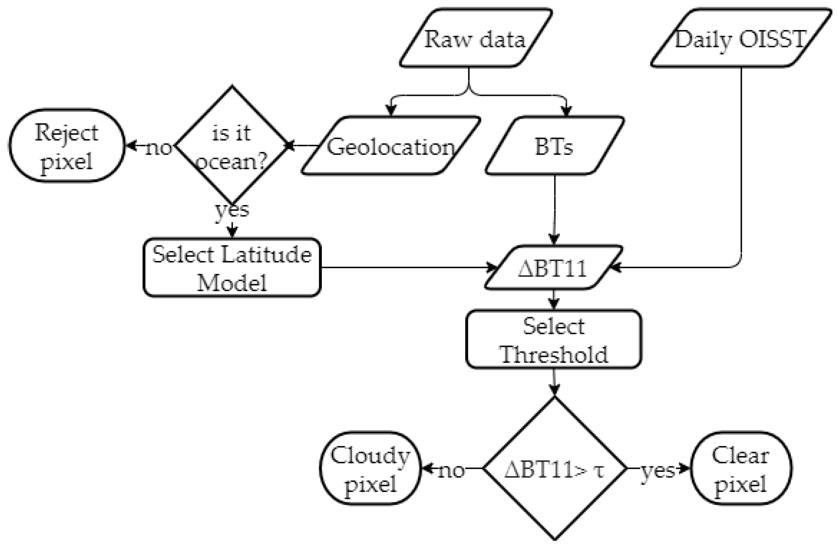
The main idea of the methodology we propose is to establish a relationship between the
, the Brightness Temperature Difference (BTD) between
and
, and the ancillary SST using a set of real images in
and
bands. The objective is to get a statistical estimation of the
as a function of the BTD and SST for clear-sky pixels. Since the
of cloudy pixels is lower than that of the clear pixels, the difference between the real and estimated
can be useful to determine the pixel state. Based on this difference, we define a threshold using a similar technique as in [
36] to determine whether the pixel is clear or cloudy.
The use of two adjacent bands has been used before in other CM algorithms [
10,
25,
36]. The methodology we propose combines the advantages of those CMs but also provides several novel ideas. First, in this work, the estimate of the
for clear sky pixels is calculated from a statistical analysis of thousands of images to consider all the atmospheric scenarios. Therefore, the
values do not depend on the performance of any radiative model or the estimate of the atmospheric conditions. Second, since our original data are
values, the CM threshold is calculated on the
value not on the SST one, as in [
25] and [
36]. Third, the threshold is not determined directly from the intersection between the distribution functions of the clear and cloudy pixels but by optimizing the results using skill scores, as explained in
Section 2.3. Finally, we include a specific analysis of partially cloudy pixels.
Although there are some pathfinders, including IR cameras, for example, the EUSO-SPB II (EUSO-Super Pressure Balloon II), the IR cameras have not provided enough images [
22]. For that reason, MODIS data have been used in this work, allowing us to develop our algorithm and validate it. Considering this CM is based on a split-window algorithm test, we have called it the Split-Window Cloudiness Mask (SWCM).
As JEM-EUSO does not retrieve the SST, a global SST model is needed. In this study, the NOAA 1/4
daily Optimum Interpolation Sea Surface Temperature (or daily OISST) [
37] provides the SST estimation.
Section 2.1 contains a short description of the data used to design and validate the algorithm.
Section 2.2 describes the fundamentals of the algorithm.
Section 2.3 details the methods to calculate the thresholds and coefficients that define the SWCM. Afterward, the results of our methodology, that is, the final coefficients and thresholds that define the SWCM and its validation, are presented in
Section 3. In
Section 4 we discuss the results attained in the previous section and compare them with those of other authors. The last section,
Section 5, provides a summary of the methodology and the main results of this work. It also includes the relevance of the results in the framework of JEM-EUSO and remote sensing in general. In this section, we also point out some future working lines oriented to combine tests of different nature in a more global CM to improve the results of individual single-test CMs.
4. Discussion
As seen in the
Section 2.3 and
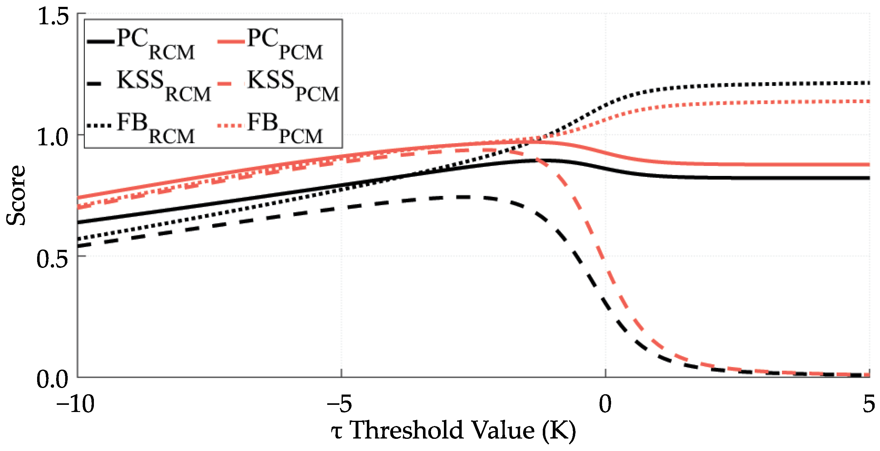
Section 3.2, different thresholds
and different performances are derived depending on the day/night state, the latitude, or season. In this section, we will discuss these results and compare them with those of other authors to better evaluate our SWCM.
As expected, the comparison with the PCM ground truth, which evaluates the performance of the SWCM to classify clear and cloudy pixels, gives more satisfactory skill scores than the comparison with the RCM ground truth, which better reflect the overall skill of the SWCM including mixed pixels. For the PCM, the , , , and take values close to one (the perfect score for those skill scores). That means that the SWCM is able to classify clear and cloudy pixels with high accuracy and that the mixed pixels are the primary source of error in the SWCM.
In general, we can say that the results are very encouraging since the
is always higher than 0.90 (including mixed pixels) for all the latitudes regardless of whether it is day or night (
Table 5). The difference in the total
score when using both ground truths is 0.08 (Tropical) and 0.07 (midlatitude), which means that the performance of the SWCM is also good in realistic scenarios, including mixed pixels.
The
presents the same behavior, with a total difference of 0.13 (tropical) and 0.7 (midlatitude). This fact reveals that the optimization of the h threshold (h = 40%) solves the issue of the
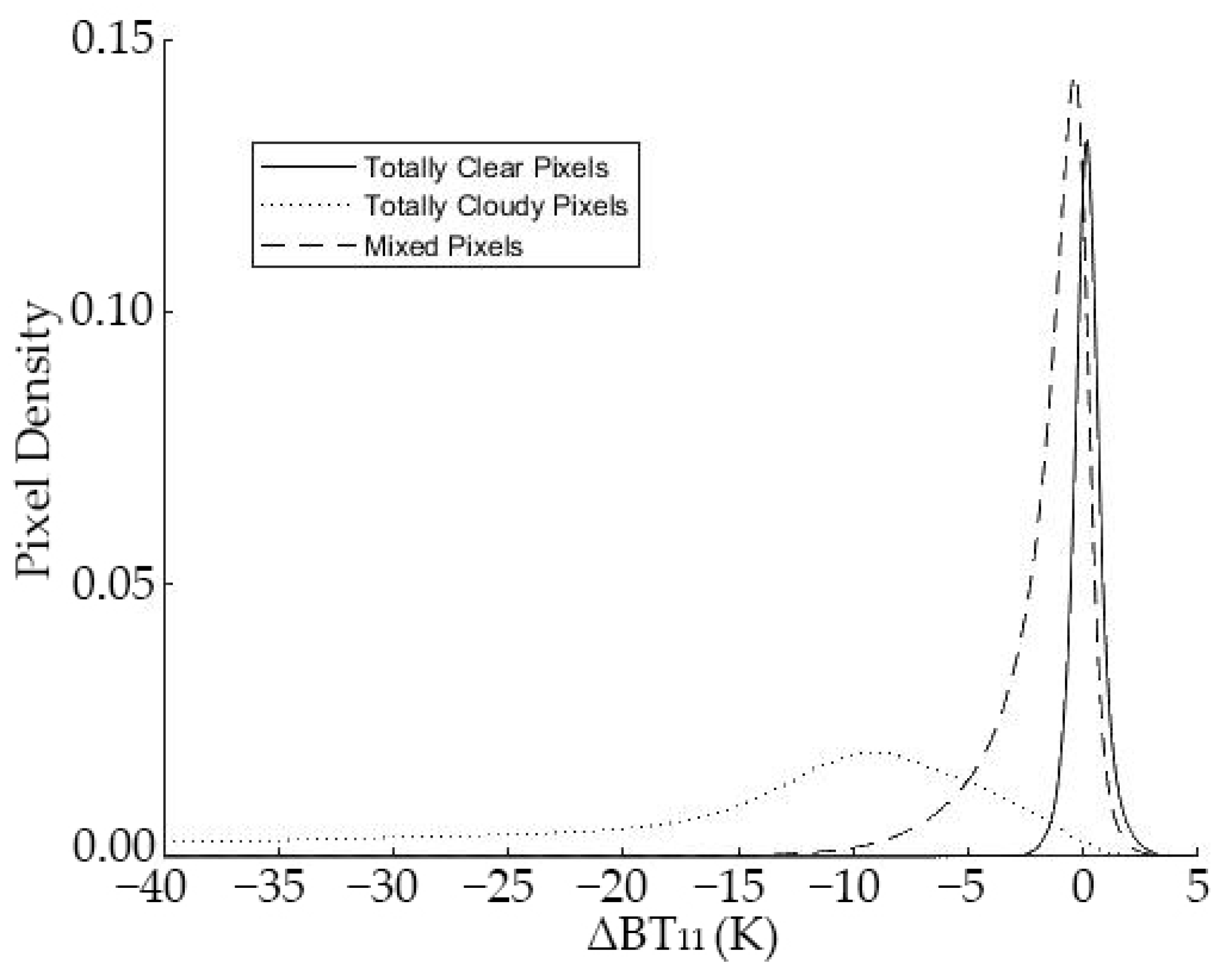
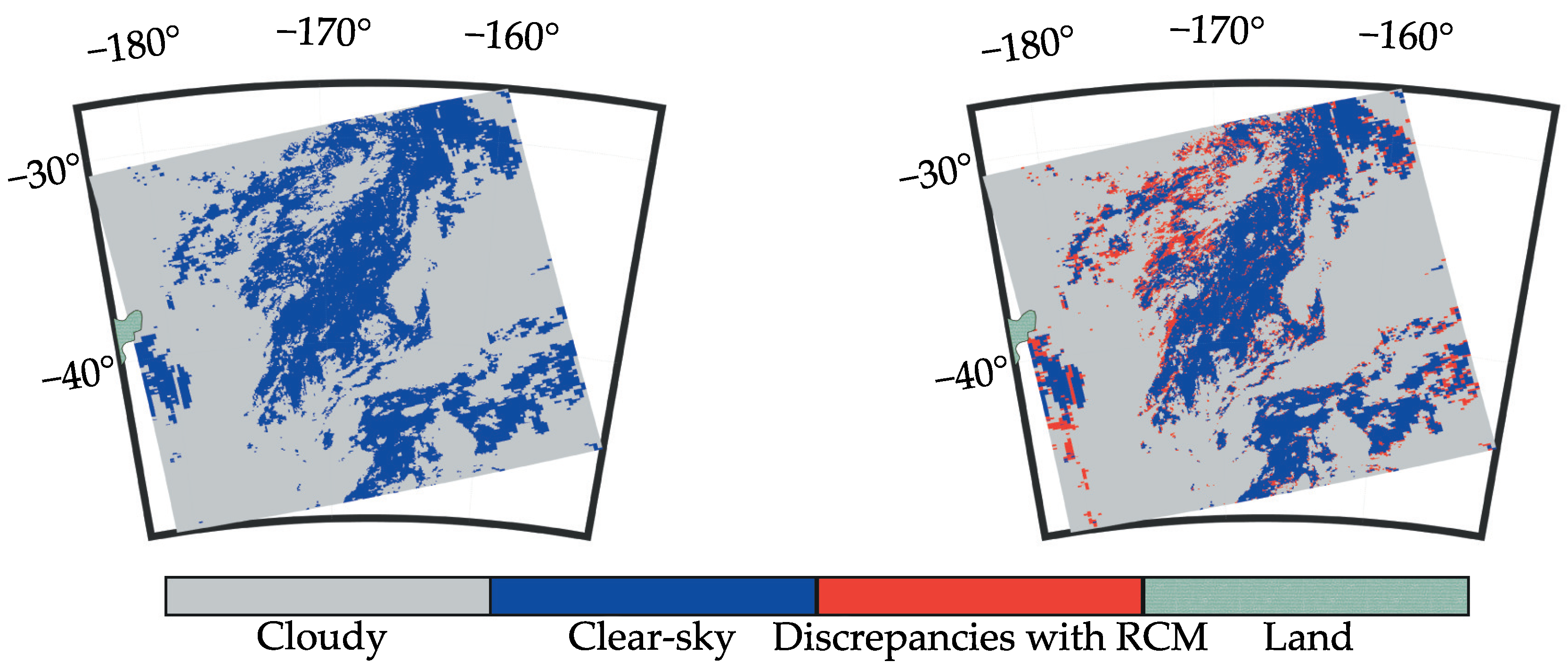
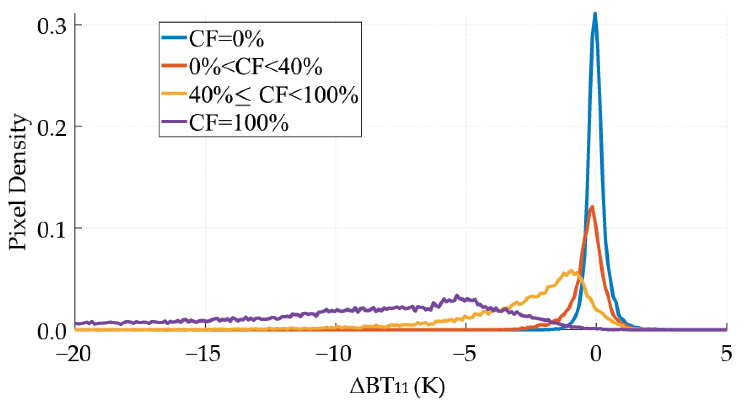
overlapping between the mixed pixels and the clear and cloudy ones, at least partially. As an illustrative example,
Figure 7 represents the probability density functions of the scene represented in
Figure 1 divided in pixels with CF below 40% and pixels with CF above 40%. In general, those mixed pixels are located in cloud edges. Nevertheless, the influence of those pixels in the SWCM performance is strong because of the size of the pixels (5 × 5 km
) that increases the percentage of pixels partially covered. Therefore, it is expected that the SWCM performance improves when applied to better spatial resolutions [
49] (as JEM-EUSO systems).
As mentioned before, the
and the
depends on the blackbody emission of the ocean (according to its temperature) and the absorption due to the atmospheric water vapour content. However,
and
calculus uses not a real SST but a daily SST provided by the NOAA Daily OISST global model. The OISST is constructed by combining observations from different platforms (satellites, ships, buoys, and Argo floats). For this reason, the OISST temperature values can differ from those of a remote sensor (±0.5 K on average [
50]). Nevertheless, if there is a bias between both temperatures for any condition (i.e., different CF conditions as shown in [
51]) the effect of those differences is minimized in the statistical procedure, that is, in the fitting process to calculate the coefficients of Equation (
1) and in the thresholds optimization.
In addition, the small diurnal SST oscillation [
52] could entail some errors that have been avoided calculating two different
for day and night (
Table 4). The difference between both
is higher for Tropical latitudes, where the SST daily oscillation is also higher. The negligible difference between the day and night values of all the scores in Tropical analysis (
Table 5) indicates that the diurnal variation is properly taken into account using different
for day and night. The midlatitude images analysis shows the same behavior except for the values of
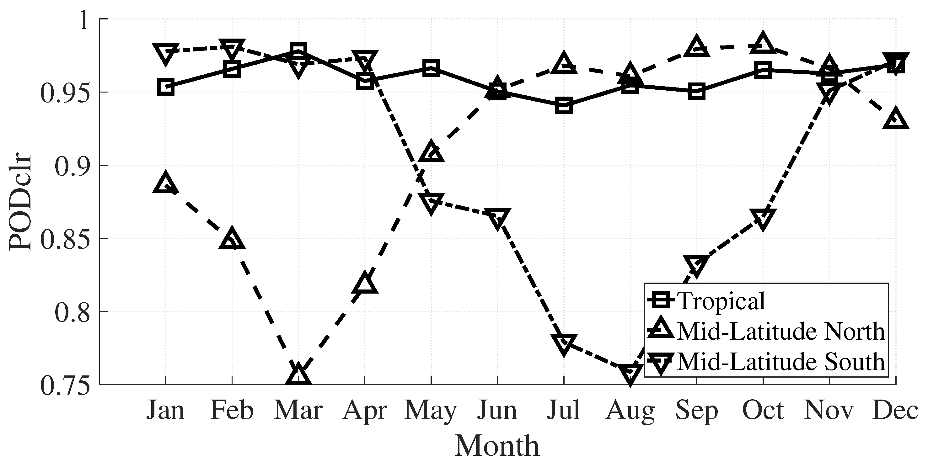
clr for which there is a clear difference between day and night. This exception could be related to the well-known difficulty of identifying clear pixels when the underlying surface is at low temperature, and there is no good contrast with clouds, which are also cold. This poor contrast between the cold SST and the clouds could also explain the seasonal variation in the midlatitude region observed in the validation section (
Section 3.2,
Table 6 and
Figure 6).
The differences between day and night performance could be associated with the variation of the atmospheric state as well. Precisely, the atmospheric vertical profiles also undergo a seasonal variation, especially the water vapor profile, which has the main responsibility for the atmospheric absorption in the TIR. Since we do not perform regression fits for each month in each geographical region, the methodology averages the atmospheric seasonal variations. As the water vapor variation occurs in the firsts kilometers of the atmosphere, it affects the
cld to a lesser extent because the clouds above the lower layers of the atmosphere can shield what happens below them. This explanation is in agreement with a lower difference between day and night
cld compared to the
clr one in the midlatitude region (
Table 5). It also agrees with a lower seasonal variation in
cld compared to
clr for the same region, as can be seen in
Table 6. However, the tropical region does not show this seasonal variation, as the water vapor content almost does not change throughout the year. Finally, the different proportions of clear and cloudy sky pixels existing could also cause the seasonal variation of the
s in the midlatitude region, e.g., for the validation subset of images, for midlatitude north, during august, the ratio between totally cloudy and clear pixels is 4.1; meanwhile, during march month, the ratio is more significant, with 6.3.
To summarize, we find slightly better results for Tropical than midlatitude regions (
Table 6). However, the skills scores are very similar between the tropical and the midlatitude cases during summer-autumn months (the discrepancies occur during the winter-spring months). In almost all cases, the
is more significant than 0.90, and the
is higher than 0.82 (Tropical) and 0.69 in the worst case of midlatitude.
In any case, to determine the scope of the SWCM in a more general framework, our results have been compared with those of other authors who also use MODIS CM as ground truth.
Table 7 contains the skills scores of different CMs when compared to MODIS CM. It should be mentioned that these comparisons do not take into account that these works cross the data of two different satellites and instruments, increasing the difference with the MODIS CM. On the contrary, this work compares the same MODIS instrument’s data to focus only on the algorithm and CM performance.
The SWCM test has been compared with a
gross test (
> threshold). The results (
Table 7) show that the results of the test used are better than the
gross test. This difference becomes greater for midlatitude, where the classification of the
gross test is poor.
The INSAT-3D Gaussian Mixture Model (GMM) CM [
39] is an algorithm that uses two TIR channels and one Middle IR (MIR) channel. It is based on the assumption that cloud data radiances are clustered in different Gaussian distributions. The CM is obtained then by merging those clusters into cloudy and clear classes.
In [
11], an operational CM for the Advanced Geostationary Radiation Imager (AGRI) on board Fengyun-4A is presented. The algorithm applies 13 spectral and spatial tests based on six different bands, producing a four-level CM product. The algorithm makes use of simulated real-time clear-sky IR radiances, using data from the Global Forecast System.
Even though the SWCM uses only one test based on two TIR bands, its global (0.91) is similar to the values of the other CMs. It is higher than the INSAT-3D GMM (0.76), although lower than the Advanced Himawari Imager (AHI) (0.93).
Concerning the , the SWCM is of the order of the others, but the SWCM is the highest. The SWCM is higher than the SWCM , unlike in the other CMs. It is noticeable that the SWCM score, which measures the ability to separate clear and cloudy pixels, is the highest one.
When analyzing the , the SWCM FAR is lower than the others, although the FAR is higher. Nevertheless, in general, all the FARs are in the same range.
Other works that show similar
scores can be found in [
53].
To summarize, the performance of the SWCM is similar to the one of the other CMs based on multispectral or spatial tests, even though the SWCM is a one-test CM based on only two spectral bands.
5. Summary and Conclusions
The main objective of this new SWCM is to provide the JEM-EUSO program with a cloudiness map in the interest regions. For this reason, we have only focused on areas over oceans because the UV principal instrument will keep clear of populated areas to avoid the associated UV light pollution.
Our proposal is a simple cloud mask test based on a split window algorithm. The inputs of the SWCM are the BTs in two spectral bands in the thermal infrared region (centered at 11 and 12 m) and SST data provided by a Global Model OISST. The method is based on two stages. The first one is an estimate of the brightness temperature of clear sky at 11 µm. The statistical procedure to calculate the estimate of is one of the novel contributions of this work. The second step calculates the difference between the estimate and the measured one. To classify the pixel, that difference is compared with a threshold. The procedure to calculate the thresholds is also novel.
The usefulness of this SWCM in the framework of JEM-EUSO is twofold. On the one hand, it will determine if there are clouds in the FoV of the UV main telescope. On the other hand, it will select the cloudy pixels where the radiative algorithms will be applied to retrieve the cloud top height, which is the main objective of the JEM-EUSO IR Camera [
54].
Concerning the resilience of the SWCM, despite the IR cameras of the different JEM-EUSO missions having slight differences in their designs (resolution, noise, altitude, etc.), the SWCM could be applied to all the JEM-EUSO pathfinders. The spectral bands (centering and width) are very similar to each other and very similar to the MODIS spectral bands. For this reason, the results obtained by applying SWCM to MODIS data can be extrapolated to the IR systems of the JEM-EUSO missions and other systems with similar spectral bands. The proximity between the bands and their coincidence with an atmospheric window also favor extrapolation. Finally, the SWCM uses brightness temperature data, which is calibrated and does not depend heavily on the sensor used.
Since the JEM-EUSO instrument is not already in orbit, we have used MODIS data. Precisely, MODIS bands #31 and #32 are very similar to those of the IR JEM-EUSO Camera. MODIS data have allowed us to develop the SWCM and validate it without crossing data between different instruments and, therefore, without introducing instrumental effects in the evaluation of the CM performance. However, in the future, these instrumental differences will have to be studied.
The SWCM results are very good when applied to totally cloudy or clear pixels, which implies that the proposed algorithm is an appropriate classifier. Comparing the results using PCM and RCM reveals that the main discrepancies are related to partially cloudy pixels at the cloud edges. However, they have been minimized by optimizing the h threshold. However, as the spatial resolution of JEM-EUSO (about 0.75 × 0.75 km) is better than the one used in this work, the expected results in the JEM-EUSO IR camera should be better. Nevertheless, those mixed pixels could also be identified and/or discarded to improve the algorithm accuracy by applying some spatial and textural techniques. The final solution will depend on the JEM-EUSO requirements.
The lower performance corresponds to the
clr for midlatitude regions during the winter months. These results could be improved by conducting specific regression fits and calculating new coefficients
A,
,
,
C, and
D for that period in midlatitude regions. Moreover, if the JEM-EUSO mission detected an EAS, local coefficients could be calculated through the radiative Transfer Equation [
11], using vertical water vapour profiles provided by numerical weather prediction models such as WRF or GFS [
55].
The scope of our study has been determined by comparing SWCM with other relevant studies. The comparison between the skill scores (
Table 7) allows us to assert that the SWCM presents a performance similar to other studies that use MOD35 data as ground truth, even though the SWCM uses just one test based on only two spectral bands.
Nevertheless, in the future, it is expected to integrate this algorithm in a more elaborated CM algorithm, also using other complementary tests. Actually, other works based on spatial analysis [
54], deep learning [
56], or Numerical Weather Forecast models [
57] have already been carried out within the JEM-EUSO community.
It is also important to emphasize the relevance of our results in the field of future remote sensing sensors. The great advantage of the proposed SWCM algorithm is its easy hardware implementation. It requires defining only two spectral bands by using band-pass interferential filters on two arrays of the same detector material. The use of only one type of material means a big simplification in terms of electronics and data acquisition and management.
Finally, we would highlight that this algorithm could also be applied to data of plenty of satellites, both operative and non-operative since the use of the TIR bands has been widespread since the second half of the last century. Moreover, the concept proposed in this article can be easily transferred to nanosatellites and CubeSats constellations devoted to Earth observation, following the current trend of development of simple and low cost, mass, and energy-consumption systems. The possibility of monitoring the presence of clouds at high resolution and in specific areas with simple systems will allow providing complementary and valuable information for numerous environmental and technological applications.


