
Symmetric Connectivity of Underwater Acoustic Sensor Networks Based on Multi-Modal Directional Transducer


 ,
,  and
and
Abstract
:1. Introduction
- 1.
- Based on the tri-modal transducer model, the optimal beamwidth of UASNs stochastically distributed near is analyzed.
- 2.
- For UASNs equipped with beamwidth directional transducer, the problem of MNCTO is formulated, which is the first attempt, to the best of our knowledge.
- 3.
- The problem of MNCTO is proved to be NP-complete by a reduction from HPHGG.
- 4.
- A volume model is introduced to denote the energy radiation, especially for omni-directional and directional models.
- 5.
- An complexity heuristic greedy algorithm is elaborated to solve the MNCTO problem.
2. Related Works
3. System Model
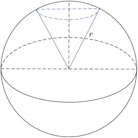
3.1. Directional Model in UASNs
3.1.1. Multi-Modal Transducer Model
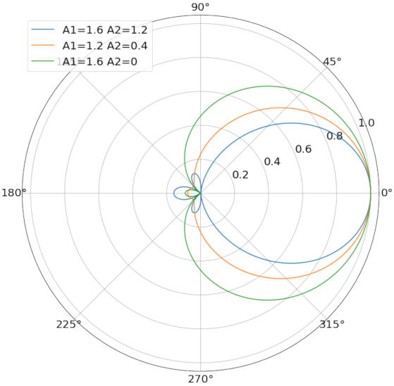
3.1.2. Optimal Beamwidth
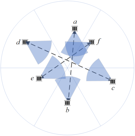
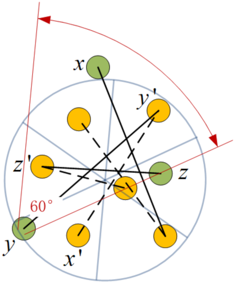
3.2. Network Model
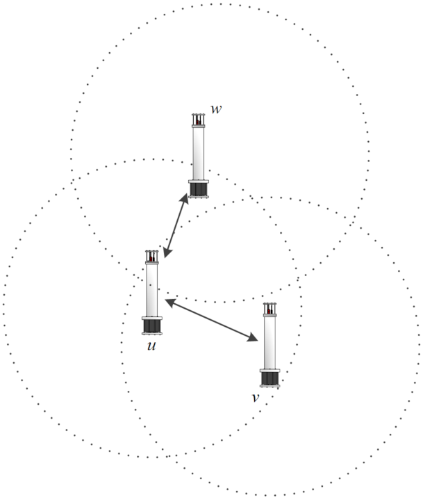
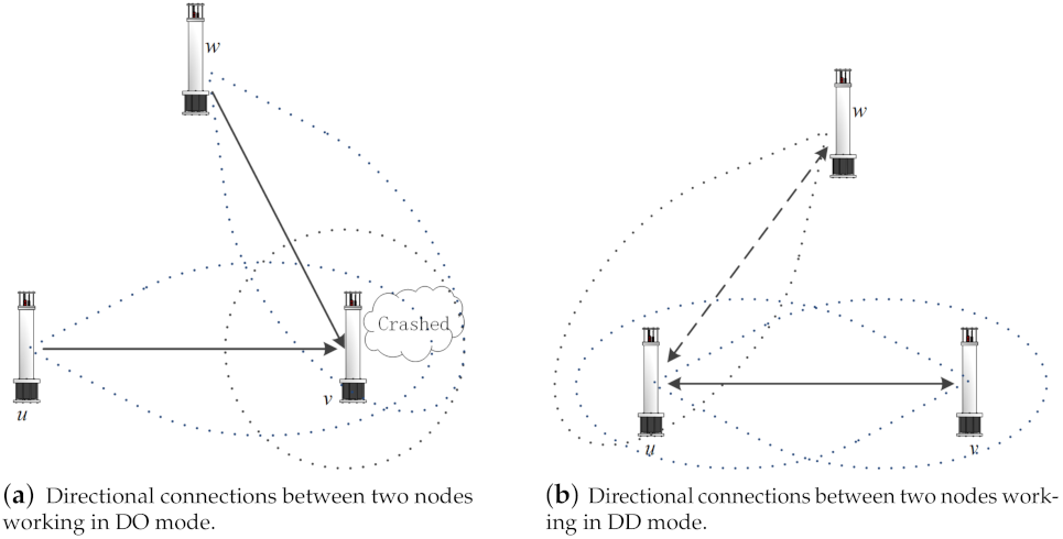
- ((respectively, ) mode: A node u transmits directionally and receives omni-directionally, or conversely. In this case, u can reach any node v as long as its beam covers the latter.
- mode: A symmetric link sets up if both the sender and receiver are orientated toward each other and they all lay within each other’s transmission range.
3.3. Energy Cost Model
4. Problem Formulation and Algorithm Proposed
4.1. Problem of Minimum Network Cost Transducer Orientation
4.1.1. NP-Complete of Transducer Orientation Problem
4.1.2. NP-Complete of MNCTO Problem
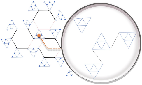
4.2. Algorithm Proposed
A Greedy Heuristic Algorithm for MNCTO
| Algorithm 1 MNCTO. |
| Input: Nodes set , Anticipated groups number |
| Output: Target groups set |
| 1: procedure Find_Tar_Groups () |
| 2: ; // Saves isolated nodes set |
| 3: ; // Target group set |
| 4: if then |
| 5: return ⌀ |
| 6: else |
| 7: ); // Clustering with K-Means |
| 8: for all do |
| 9: if contains more than 9 nodes then |
| 10: ); // Get the centroid of the group |
| 11: ; |
| 12: partition g into 6 sectors; |
| 13: if g has a target group then |
| 14: ; |
| 15: ; |
| 16: else |
| 17: Sorting with asending order for all its vertexes |
| 18: for all do |
| 19: ); |
| 20: ); // Rotate g with anti-clockwise |
| 21: if g has a target group then |
| 22: ; |
| 23: ; |
| 24: break; |
| 25: end if |
| 26: end for |
| 27: ; |
| 28: end if |
| 29: else |
| 30: ; |
| 31: end if |
| 32: end for |
| 33: if then // In order for convergence |
| 34: |
| 35: else |
| 36: |
| 37: end if |
| 38: return ; // Recursion |
| 39: end if |
| 40: end procedure |
| Algorithm 2 MNCTO. |
| Input: Target group , Rotating Angle |
| Output: Rotated target group |
| 1: procedure RotateA () |
| 2: for all do |
| 3: |
| 4: Re-calculate for |
| 5: resets for |
| 6: end for |
| 7: return |
| 8: end procedure |
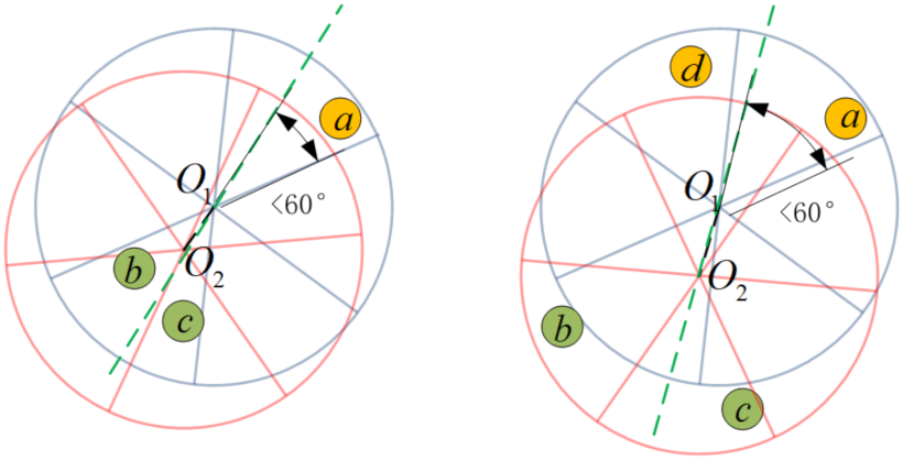
- Case 1:
- Case 2:
| Algorithm 3 MNCTO. |
| Input: Target groups , Isolated nodes |
| Output: Void |
| 1: procedure Establish_Full_Connections () |
| 2: |
| 3: // Establish MST for centers |
| 4: for all do |
| 5: for all do // link target group with peers |
| 6: if not then |
| 7: link with |
| 8: end if |
| 9: end for |
| 10: for all do // link with |
| 11: if then |
| 12: link with its peer // peer: node locating in opposite sector |
| 13: end if |
| 14: end for |
| 15: for all do // link themselves |
| 16: find corresponding to the smallest angle |
| 17: link with other 2 |
| 18: end for |
| 19: end for |
| 20: for all do // link outliers with their nearest target group |
| 21: |
| 22: |
| 23: for all do |
| 24: if then |
| 25: |
| 26: |
| 27: end if |
| 28: link with |
| 29: end for |
| 30: end for |
| 31: end procedure |
5. Simulation Evaluations
5.1. Performance Metrics
- Network Energy Cost ()The energy consumed by a network originates from packets delivered from the source node to sink node. In ad hoc networks, all nodes are homogeneous and able to act as at least one of sender/relay/sink, so the metric is defined to evaluate the energy efficiency, as shown below:where random packet paths are counted, in denote arbitrary two stochastic nodes and implies that the cost is positively correlated to the spreading distance (see Equation (18)), where k denotes the spreading factor that ranges from 1 to 2 in an underwater environment; thus a median of 1.5 is used. In addition, needs to be weighted when compared with the omni-directional mode, and should be normalized by a common constant; thus the network deployment boundary is chosen.
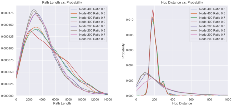
- Delivery Distance DistributionAs the term suggests, this metric counts the distribution of traveling distances of large quantities of packets with random source and sink, which is actually another enhanced metric of network energy consumption that presents key performance intuitively.
- Average Single Hop Distance()It indicates the average link distance, and can be measured as Equation (25), where denotes the traveling path length of a random packet, while denotes the hops number between .
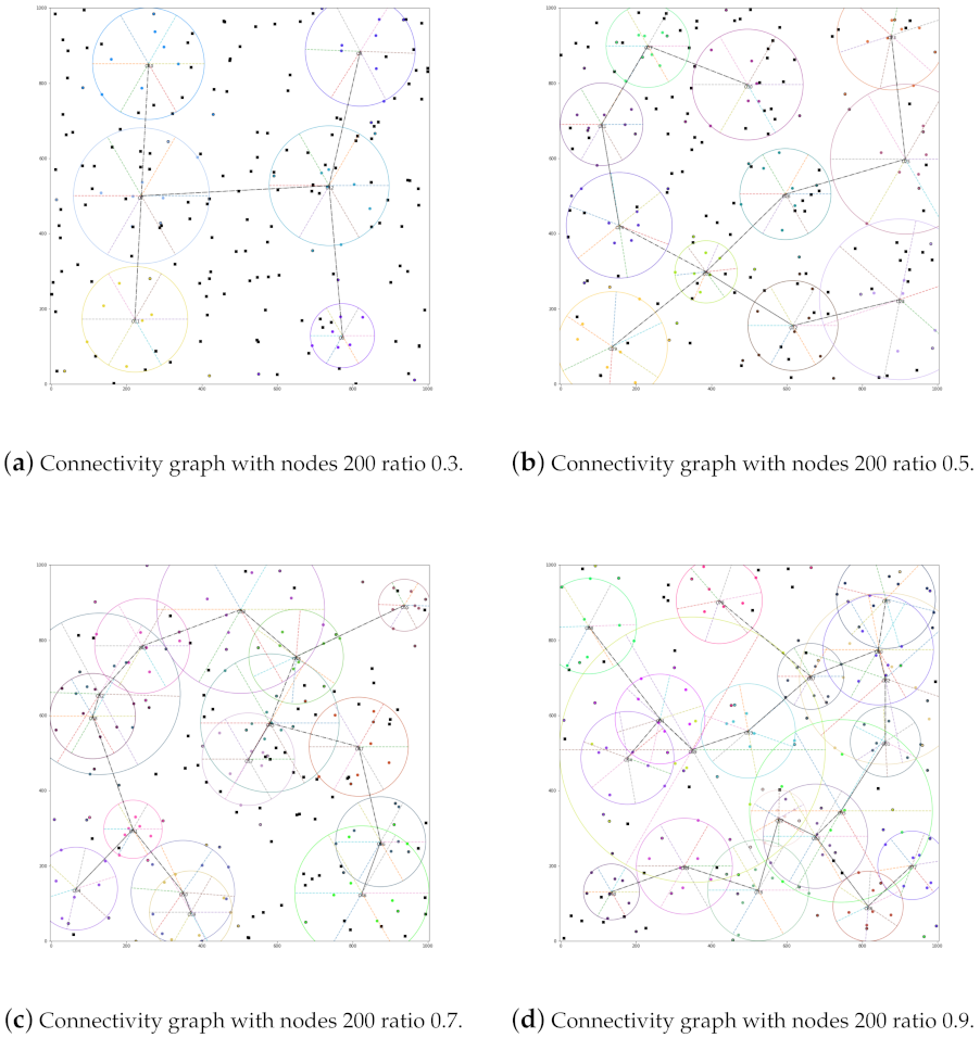
5.2. Simulation Performance
6. Conclusions
Author Contributions
Funding
Institutional Review Board Statement
Informed Consent Statement
Data Availability Statement
Acknowledgments
Conflicts of Interest
Appendix A
References
- Shahabudeen, S.; Motani, M.; Chitre, M. Analysis of a High-Performance MAC Protocol for Underwater Acoustic Networks. IEEE J. Ocean. Eng. 2014, 39, 74–89. [Google Scholar] [CrossRef]
- Su, Y.; Guo, L.; Jin, Z.; Fu, X. A Voronoi-Based Optimized Depth Adjustment Deployment Scheme for Underwater Acoustic Sensor Networks. IEEE Sens. J. 2020, 20, 13849–13860. [Google Scholar] [CrossRef]
- Zhang, Y.; Sun, D.; Zhang, D. Robust adaptive acoustic vector sensor beamforming using automated diagonal loading. Appl. Acoust. 2009, 70, 1029–1033. [Google Scholar] [CrossRef]
- Liang, G.; Shi, Z.; Qiu, L.; Sun, S.; Lan, T. Sparse Bayesian Learning Based Direction-of-Arrival Estimation under Spatially Colored Noise Using Acoustic Hydrophone Arrays. J. Mar. Sci. Eng. 2021, 9, 127. [Google Scholar] [CrossRef]
- Heidemann, J.; Stojanovic, M.; Zorzi, M. Underwater sensor networks: Applications, advances and challenges. Philos. Trans. 2012, 370, 158. [Google Scholar] [CrossRef]
- Xie, P.; Cui, J.H. Exploring random access and handshaking techniques in large-scale underwater wireless acoustic sensor networks. In Proceedings of the MTS/IEEE Oceans, Boston, MA, USA, 18–21 September 2006; pp. 1–6. [Google Scholar]
- Petroccia, R.; Petrioli, C.; Potter, J. Performance Evaluation of Underwater Medium Access Control Protocols: At-Sea Experiments. IEEE J. Ocean. Eng. 2017, 43, 547–556. [Google Scholar] [CrossRef]
- Min, K.P.; Rodoplu, V. UWAN-MAC: An energy-efficient MAC protocol for underwater acoustic wireless sensor networks. IEEE J. Ocean. Eng. 2007, 32, 710–720. [Google Scholar]
- Emokpae, L.; Younis, M. Reflection-enabled directional MAC protocol for underwater sensor networks. In Proceedings of the Wireless Days, Niagara Falls, ON, Canada, 10–12 October 2011. [Google Scholar]
- Butler, J.L.; Butler, A.L.; Rice, J.A. A tri-modal directional transducer. J. Acoust. Soc. Am. 2004, 115, 658–665. [Google Scholar] [CrossRef] [PubMed]
- Akhtar, A.; Ergen, S.C. Directional MAC protocol for IEEE 802.11ad based wireless local area networks. Adhoc. Netw. 2017, 69, 49–64. [Google Scholar] [CrossRef]
- Liu, H.; Liu, Z.; Li, D.; Lu, X.; Du, H. Approximation algorithms for minimum latency data aggregation in wireless sensor networks with directional antenna-ScienceDirect. Theor. Comput. Sci. 2013, 497, 139–153. [Google Scholar] [CrossRef]
- Ai, J.; Abouzeid, A.A. Coverage by directional sensors in randomly deployed wireless sensor networks. J. Comb. Optim. 2006, 11, 21–41. [Google Scholar] [CrossRef] [Green Version]
- Pu, Q.; Hwang, W.J. Adaptive Power Control for MAC Protocol in Ad Hoc Network with Directional Antennas. SIAM J. Control. Optim. 2008, 29, 1061–1090. [Google Scholar]
- Liu, B.; Lei, J. Principles of Underwater Acoustics; Harbin Engineering University Press: Harbin, China, 2010. [Google Scholar]
- Casari, P.; Zorzi, M. Protocol design issues in underwater acoustic networks. Comput. Commun. 2011, 34, 2013–2025. [Google Scholar] [CrossRef]
- Khalid, M.; Ullah, Z.; Ahmad, N.; Arshad, M.; Jan, B.; Cao, Y.; Adnan, A. A Survey of Routing Issues and Associated Protocols in Underwater Wireless Sensor Networks. J. Sens. 2017, 2017, 7539751. [Google Scholar] [CrossRef]
- Arkin, E.M.; Fekete, S.P.; Islam, K.; Meijer, H.; Mitchell, J.; Polishchuk, V.; Rappaport, D.; Xiao, H. Not being (super)thin or solid is hard: A study of grid Hamiltonicity. Comput. Geom. Theory AMP Appl. 2009, 42, 582–605. [Google Scholar] [CrossRef] [Green Version]
- Li, L.; Halpern, J.Y.; Bahl, P.; Wang, Y.M.; Wattenhofer, R. A cone-based distributed topology-control algorithm for wireless multi-hop networks. IEEE/ACM Trans. Netw. (TON) 2005, 13, 147–159. [Google Scholar] [CrossRef]
- Aschner, R.; Katz, M.J.; Morgenstern, G. Symmetric Connectivity with Directional Antennas. Comput. Geom. 2011, 46, 1017–1026. [Google Scholar] [CrossRef]
- Aschner, R.; Katz, M.J. Bounded-Angle Spanning Tree: Modeling Networks with Angular Constraints. Int. Colloq. Autom. Lang. Program. 2014, 77, 349–373. [Google Scholar]
- Carmi, P.; Katz, M.J.; Lotker, Z.; Rosen, A. Connectivity guarantees for wireless networks with directional antennas. Comput. Geom. Theory Appl. 2011, 44, 477–485. [Google Scholar] [CrossRef] [Green Version]
- Dobrev, S.; Eftekhari, M.; Macquarrie, F.; Maňuch, J.; Ponce, O.M.; Narayanan, L.; Opatrny, J.; Stacho, L. Connectivity with directional antennas in the symmetric communication model. Comput. Geom. Theory Appl. 2016, 55, 1–25. [Google Scholar] [CrossRef]
- Bose, P.; Carmi, P.; Damian, M.; Flatland, R.; Katz, M.J.; Maheshwari, A. Switching to Directional Antennas with Constant Increase in Radius and Hop Distance. Algorithmica 2014, 69, 397–409. [Google Scholar] [CrossRef]
- Kranakis, E.; Macquarrie, F.; Ponce, O.M. Connectivity and stretch factor trade-offs in wireless sensor networks with directional antennae. Theor. Comput. Sci. 2015, 590, 55–72. [Google Scholar] [CrossRef]
- Tran, T.; Min, K.A.; Huynh, D.T. Establishing symmetric connectivity in directional wireless sensor networks equipped with 2π/3 antennas. J. Comb. Optim. 2017, 34, 1029–1051. [Google Scholar] [CrossRef]
- Chen, Z.; Qiao, G.; Zhou, F.; Niaz, A. High-precision Localization Correction Method for Underwater Unknown Target with single Floating anchor node. IET Radar Sonar Navig. 2020, 14, 1494–1501. [Google Scholar]
- Li, J.; Andrew, L.; Foh, C.H.; Zukerman, M.; Chen, H.H. Connectivity, Coverage and Placement in Wireless Sensor Networks. Sensors 2009, 9, 7664–7693. [Google Scholar] [CrossRef] [PubMed] [Green Version]
- Du, J.; Kranakis, E.; Ponce, O.M.; Rajsbaum, S. Neighbor Discovery in a Sensor Network with Directional Antennae. Ad Hoc Sens. Wirel. Netw. 2016, 30, 261–286. [Google Scholar]
- Stojanovic, M. On the relationship between capacity and distance in an underwater acoustic communication channel. ACM Sigmobile Mob. Comput. Commun. Rev. 2007, 11, 34–43. [Google Scholar] [CrossRef]
- Xue, F.; Kumar, P.R. The Number of Neighbors Needed for Connectivity of Wireless Networks. Wirel. Netw. 2004, 10, 169–181. [Google Scholar] [CrossRef]


| Beamwidth | Mode | Range | Complexity | Reference |
|---|---|---|---|---|
| Fixed Orientation | Not always guaranteed | NPC | [22] | |
| Fixed Orientation | [20] | |||
| Fixed Orientation | 7 | [24] | ||
| Fixed Orientation | [25] | |||
| Fixed Orientation | 5 | [26] | ||
| Fixed Orientation | [25] | |||
| Fixed Orientation | [23] |
| Parameter | Network Type | |
|---|---|---|
| UADSNs | UASNs | |
| Connection Algorithm | MNCTO | UDG |
| Deployment Range | 1000 × 1000 | 1000 × 1000 |
| Number of Nodes | 100–400 | 100–400 |
| Clustering Ratio | 0.2–1.0 | - |
| Transmission Range | - | [150, 200, 250, 300] |
| Unit Distance Energy Cost | 1 | 14.93 |
| Routing Aigorithm | Dijkstra | Dijkstra |
Publisher’s Note: MDPI stays neutral with regard to jurisdictional claims in published maps and institutional affiliations. |
© 2021 by the authors. Licensee MDPI, Basel, Switzerland. This article is an open access article distributed under the terms and conditions of the Creative Commons Attribution (CC BY) license (https://creativecommons.org/licenses/by/4.0/).
Share and Cite
Qiao, G.; Liu, Q.; Liu, S.; Muhammad, B.; Wen, M. Symmetric Connectivity of Underwater Acoustic Sensor Networks Based on Multi-Modal Directional Transducer. Sensors 2021, 21, 6548. https://doi.org/10.3390/s21196548
Qiao G, Liu Q, Liu S, Muhammad B, Wen M. Symmetric Connectivity of Underwater Acoustic Sensor Networks Based on Multi-Modal Directional Transducer. Sensors. 2021; 21(19):6548. https://doi.org/10.3390/s21196548
Chicago/Turabian StyleQiao, Gang, Qipei Liu, Songzuo Liu, Bilal Muhammad, and Menghua Wen. 2021. "Symmetric Connectivity of Underwater Acoustic Sensor Networks Based on Multi-Modal Directional Transducer" Sensors 21, no. 19: 6548. https://doi.org/10.3390/s21196548
APA StyleQiao, G., Liu, Q., Liu, S., Muhammad, B., & Wen, M. (2021). Symmetric Connectivity of Underwater Acoustic Sensor Networks Based on Multi-Modal Directional Transducer. Sensors, 21(19), 6548. https://doi.org/10.3390/s21196548