Improved RRT-Connect Algorithm Based on Triangular Inequality for Robot Path Planning

Abstract

This paper proposed a triangular inequality-based rewiring method for the rapidly exploring random tree (RRT)-Connect robot path-planning algorithm that guarantees the planning time compared to the RRT algorithm, to bring it closer to the optimum. To check the proposed algorithm’s performance, this paper compared the RRT and RRT-Connect algorithms in various environments through simulation. From these experimental results, the proposed algorithm shows both quicker planning time and shorter path length than the RRT algorithm and shorter path length than the RRT-Connect algorithm with a similar number of samples and planning time.

1. Introduction

With the recent Fourth Industrial Revolution, interest in mobile robots has increased in various fields such as robotics, smart factories, and autonomous driving [1]. Classical mobile robot path-planning algorithms can be classified into three broad categories [2]. The first is the road map approach algorithm [3], which is easy to implement by designing a map that represents a path that can be moved and plan through it. The second is cell decomposition algorithm [4], which creates a path by dividing the configuration space into cells and connecting each cell using a graph. The last is the artificial potential field algorithm [5], which creates an artificial potential field and directs the robot to the goal according to the flow of potential power.

‘Optimality’ means always ensuring the optimal path. ‘Clearance’ indicates a lower probability of collision between obstacles and the robot. ‘Completeness’ means that if a path exists, it can always be found. Optimality, clearance, and completeness are considered important in these classical algorithms and have been the main focus of study [6]. Particularly if completeness is not guaranteed by the robot path-planning algorithm, there is a problem that the path may not be found in finite time. This is a fatal problem in robot path planning.

Recently, sampling-based path-planning algorithms [7,8,9,10,11,12] such as rapidly exploring random tree (RRT) [13], which is quicker and less computationally intensive than classical algorithms, have been attracting attention. The main purpose of sampling-based algorithms is to find a path that can reach the goal as quickly as possible using randomly extracted sample points (random sampling). Unlike classical algorithms, sampling-based algorithms have difficulty fully reflecting the optimality and completeness. Therefore, most sampling-based algorithms claim ‘Probabilistic completeness’, which explains that they can be probabilistically close to complete when random sampling is repeated infinitely [14]. This means that it is difficult to guarantee the ‘Planning time’ (first path finding time), which refers to how quickly the path can be planned from the start point to the goal point, and the ‘Convergence rate’, which means iterative sampling to bring the path closer to the optimum after the first path has been found. If the situation does not allow enough time to plan the path, it can create a path that is more different from the optimal path. Even so, the sampling-based algorithm is mainly used in dynamic environments because it enables quicker path planning with very little planning time compared to classical algorithms.

To overcome these limitations of planning time and convergence rate, many studies are being conducted to expand the RRT algorithm. The RRT-Connect [15] algorithm finds a connected path more quickly than the RRT algorithm by setting the start point and goal point as the roots of separate trees and expanding both trees alternately. In addition, there are algorithms that optimize paths based on the principle of triangular inequality, such as RRT*-Smart algorithm [16] and Quick-RRT* algorithm [17], to derive a path that is close to the optimal. Many algorithms [18,19,20,21] that extend the RRT algorithm have been studied.

The above algorithms show more efficient performance by improving the RRT algorithm to overcome the limitations of sampling-based methods but they are still not perfect. Their limitations include being unable to derive the optimal length and there is room for improvement in terms of the number of operations and time. For example, the RRT* algorithm has rewiring(search for the parent node as a via point nearby a newly inserted node, where the addition of path length from the start point to the via point and path length from the via point to the newly inserted node in the tree is the optimized, and change the neighboring nodes to optimize the path length) and neighbor search (search for nodes nearby the node to be newly inserted in the tree) processes to obtain shorter path lengths than the RRT algorithm [18]. However, there is an efficiency trade-off in this process. In other words, while the convergence rate has improved, the planning time has significantly increased [22]. Therefore, the RRT* algorithm cannot be said to be better than the RRT algorithm in all performance metrics and it can be said that the RRT* algorithm gets closer to the optimum at the expense of planning time.

To overcome the limitation of getting closer to the optimum at the expense of planning time, this paper proposes a triangular inequality-based RRT-Connect algorithm that finds an ancestor node as a via point, where the addition of path length from the start point to the via point and path length from the via point to the newly inserted node is the most optimized, based on the principle of triangular inequality and RRT-Connect. The proposed algorithm shortens the planning time while also pursuing optimization through rewiring. In addition, we will verify the efficiency by comparing the RRT and RRT-Connect algorithms from previous studies through simulation experiments. As a result, this paper shows that the proposed algorithm has a shorter path length than the RRT and RRT-Connect algorithms without sacrificing other performance measures such as the number of samples or planning time.

The scope of the research we will cover is how much more quickly it can find the path and how much shorter the path is. This is because in a dynamic environment, it is more important to find a navigable path. In a dynamic environment, there may not be enough time for convergence. In other words, the purpose of our proposed algorithm is to improve the RRT-Connect algorithm so that it can find a shorter path over the same planning time (computation time before convergence or computation time for first path finding).

Figure 1 shows an overview of the three main algorithms covered in this paper: RRT, RRT-Connect, and the proposed algorithm. In this figure, the start q_start and goal points are q_goal, respectively. The RRT algorithm in Figure 1a shows that the path is expanded in a tree structure and the RRT-Connect algorithm in Figure 1b shows that the trees that are expanded at the start and goal points attract and connect each other. The proposed algorithm in Figure 1c shows that the RRT-Connect algorithm was rewired into a triangular inequality during path planning.

In this paper, Section 2 introduces the RRT algorithm, Section 3 introduces the RRT-Connect algorithm, and the triangular inequality-based RRT-Connect algorithm is proposed in Section 4. In detail, Section 4.1 shows the pseudocode of the proposed rewiring method through the principle of triangular inequality, which can be applied to the RRT-Connect algorithm, Section 4.2 shows the mathematical modeling of the proposed algorithm, Section 4.3 and Section 4.4 show the pseudocode of each method of the RRT-Connect algorithm applying the proposed rewiring method, and Section 4.5 shows the path-planning process for the proposed algorithm that applies the proposed rewire method to the RRT-Connect algorithm. Section 5 shows the experimental environment and results to check the performance of the proposed algorithm and Section 6 presents the conclusion.

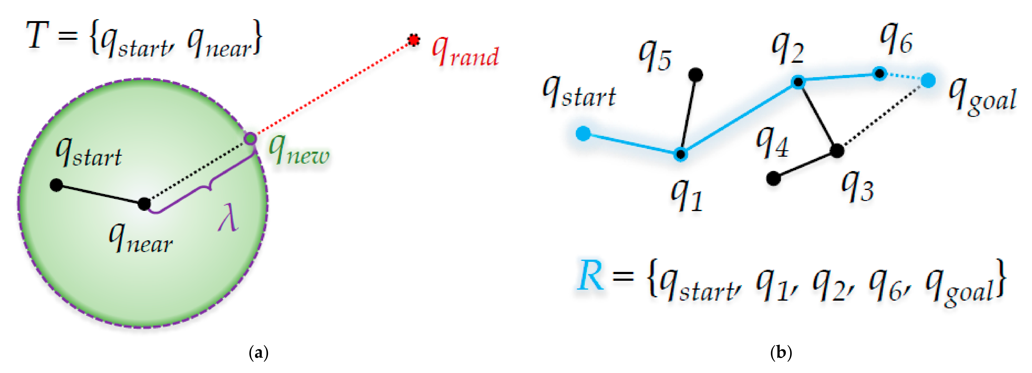
2. Rapidly Exploring Random Tree (RRT) Algorithm

Rapidly exploring Random Tree (RRT) algorithm [13] is the most representative sampling-based path-planning algorithm. The RRT algorithm plans a path by gradually expanding a tree with a root node at the start point using random sampling. It is designed to handle non-holonomic constraints and high degrees of freedom [12].

When a random sample is generated in the configuration space, it tries to connect at a point separated by a preset step length from the node nearest to the random sample among nodes constituting the tree with the step length. If tree connections are possible, nodes are added to create an extended tree.

As mentioned in the introduction, this sampling-based path-planning algorithm uses randomly generated sample points to find a path that can reach the goal as quickly as possible, so it is difficult to sufficiently reflect the optimality and completeness.

Figure 2 shows the path-planning process of the RRT algorithm. Figure 2a shows that q_new is created at the node position q_near of the tree T nearest to the random sample position q_rand. Figure 2b shows the resultant path R among several candidate paths to the start position q_start and the goal position q_goal.

3. RRT-Connect Algorithm

Path planning through the RRT algorithm may have a disadvantage in that since random samples appear with the same probability in all regions, the tree easily extends even in a direction irrespective of the goal, resulting in a long planning time and inefficiency. The RRT-Connect algorithm [15] proposed later has two new ideas as the method to compensate for the disadvantage of the RRT algorithm.

The first is that the start and goal points are each inserted as root nodes and extended in each direction alternately. The two trees extending from the start point and the goal point expand as if attracting one another (which prevents the tree and is a disadvantage of the RRT algorithm) is in a direction irrespective of the goal. This enhances the disadvantage of the planning time required to search for a path. The second is the concept of ‘Extend’, which continues extending to the other side of the tree if there are no collisions with obstacles when the tree extends. Through this, unlike the RRT algorithm that extends the maximum extension length when the sample is generated and is inserted into the tree, the tree continues to expand in the direction of the goal if there is no collision with an obstacle, so the path can be planned more quickly.

Path planning through the RRT-Connect algorithm can find a path quicker than the RRT algorithm, but the ‘Extend’ method does not work properly in complex environments with narrow paths and many obstacles and it can be difficult. In addition, the path planned using the RRT-Connect algorithm is far from the optimal length, so it does not properly reflect optimality.

3.1. Pseudocode of the RRT-Connect Algorithm

This section shows the pseudocode of the RRT-Connect algorithm used in the experiment in this paper that was designed based on [15] in which the RRT-Connect algorithm was proposed. The RRT-Connect algorithm can be represented by a main algorithm (A1) and two main methods (A2 and 3).

Algorithm 1 shows the pseudocode of RRT-Connect algorithm. Both of the two initial trees T_a and T_b have q_start and q_goal as root nodes and these two trees randomly sample N times and aim to reach each other during their expansion. Unlike RRT, the RRT-Connect algorithm is divided into two methods: ‘Extend’ and ‘Connect’. The ‘Extend’ method (A2) creates q_new from q_rand in T_a and extends from T_b to the q_new direction of T_a, and the ‘Connect’ method (A3) determines whether the two trees T_a and T_b have reached each other; if they do, merge them into one tree to obtain a path P_reach between the root nodes q_start and q_goal of the two trees.

Algorithm 1 Pseudocode of the RRT-Connect Algorithm
Input: qstart ← Start Point Position qgoal ← Goal Point Position λ ← Step Length C ← Position Set of All Boundary Points in All Obstacles Ν ← Number of Random Samples Output: R ← Result of Path R Initialize: Ta ← Null Tree Tb ← Null Tree dshorter ← 0
BeginRRT-ConnectProcedure
1	Ta ← Insert Root Node<qstart> to Ta
2	Tb ← Insert Root Node<qgoal> to Tb
3	While 1 ← n to N do
4	Generate n-th Random Sample
5	qrand ← Position of n-th Random Sample
6	If Not Extend(Ta, Tb, qnewB ← Null, qrand, λ, C) then
7	If Connect(Preach ← Null Path, Ta, Tb, qnewB, λ) then
8	dreach ← Distance of Preach
9	If dshorter = 0 or dshorter > dreach then
10	R ← Preach
11	dshorter ← dreach
12	Swap(Ta, Tb)
EndRRT-ConnectProcedure

When a path is created by the ‘Connect’ method, the distance d_reach is calculated for the path P_reach from q_start to q_goal. At this time, if d_reach is smaller than d_shorter (the shortest path length until now) or P_reach is the first path found (i.e., d_shorter = 0), the resultant path R becomes P_reach, and d_shorter becomes d_reach. At the end of the next N sampling, R becomes the final planned path. If the number of random sampling remains, the above process is repeated.

3.2. Pseudocode of the Extend Method from the RRT-Connect Algorithm

This section introduces the ‘Extend’ method used in pseudocode (A1) of the RRT-Connect algorithm in Section 3.1.

Algorithm 2 shows the pseudocode of the ‘Extend’ method in the RRT-Connect algorithm. The isInside function determines whether q_rand is inside a circle (or n-sphere) with the node position q_near of the tree T_a nearest the q_rand position as the center and λ as the radius. If it is not located inside (False), q_newA becomes the intersection of the circle (or n-sphere) with q_near as the center and λ as the radius, and the line segment connecting q_rand and q_near. If it is determined that there is no obstacle between q_newA and q_near by the isTrapped function (False), q_newA is inserted into the tree as a child node of q_near of T_a. If there is an obstacle (True), the ‘Extend’ method returns True (f_trap) and terminates. Otherwise, it proceeds with the remaining process and returns False (f_trap) when the process ends.

Algorithm 2 Pseudocode of the original ‘Extend’ method from the RRT-Connect Algorithm
Input: Ta ← Tree Ta from RRT-Connect Tb ← Tree Tb from RRT-Connect qnewB ← Position qnewB from RRT-Connect qrand ← Position qrand from RRT-Connect λ ← Step Length λ from RRT-Connect C ← Position Set C from RRT-Connect Output: ftrap ← Result of Boolean ftrap Ta ← Result of Tree Ta //Return by Reference Tb ← Result of Tree Tb //Return by Reference qnewB ← Result of Position qnewB //Return by Reference Initialize: ftrap ← False
Begin ExtendProcedure fromRRT-Connect
1	qnear ← Find Position of Nearest Node in Ta from qrand
2	If NotisInside(qnear, qrand, λ) then
3	qnewA ← Position of the Intersection Point between the Line Segment connecting qrand and qnear and a Circle with Radius λ centered at qnear //2D: Circle, 3D: Sphere, …
4	Else
5	qnewA ← qrand
6	IfisTrapped(qnewA, qnear, C) then
7	ftrap ← True
8	Else
9	Ta ← Insert Node<qnewA> and Edge<qnewA, qnear> to Ta
10	qnear ← Find Position of Nearest Node in Tb from qnewA
11	If isInside(qnear, qnewA, λ) then
12	qnewB ← qnear
13	Else
14	qnewB ← Position of Intersection Point between Line Segment connecting qnewA and qnear, and Circle with Radius λ centered at qnear //2D: Circle, 3D: Sphere, …
15	While Not isTrapped(qnewB, qnear, C) do
16	Tb ← Insert Node<qnewB> and Edge<qnewB, qnear> to Tb
17	If Not isInside(qnewA, qnewB, λ) then
18	qnear ← qnewB
19	qnewB ← Position of Intersection Point between Line Segment connecting qnewA and qnear, and Circle with Radius λ centered at qnear //2D: Circle, 3D: Sphere, …
20	Else
21	Break
EndExtendProcedure fromRRT-Connect

This is the process of making T_a and T_b reach each other: First, the node T_b nearest to q_newA becomes the new q_near. At this time, using the isInside function, it is determined whether q_newA is inside a circle (or n-sphere) with q_near as the center and λ as the radius, and if it is located inside (True), q_newB becomes q_near and is located inside. If not (False), q_newB becomes the intersection of the circle (or n-sphere) with q_near as the center and λ as the radius and the line segment connecting q_newA and q_near. If q_newB is created, then the following process is repeated until it can determine whether there is an obstacle between q_newB and q_near by the isTrapped function and if there is the obstacle between them (True) or if q_newB reaches q_newA by the isInside function.

If there is no obstacle between q_newB and q_near (False), insert q_newB into T_b as a child node of q_near. At this time, if the isInside function determines that q_newB has not reached the λ radius with q_newA as the center (False), q_near becomes q_newB and a new q_newB will created from this q_near.

Figure 3 shows the ‘Extend’ method in the RRT-Connect algorithm. In detail, it shows that the first q_newA is created, and q_newB is created with radius of length λ in the direction of q_newA from the q_near position in the figure. Clearly, T_b extends in the T_a direction for reach.

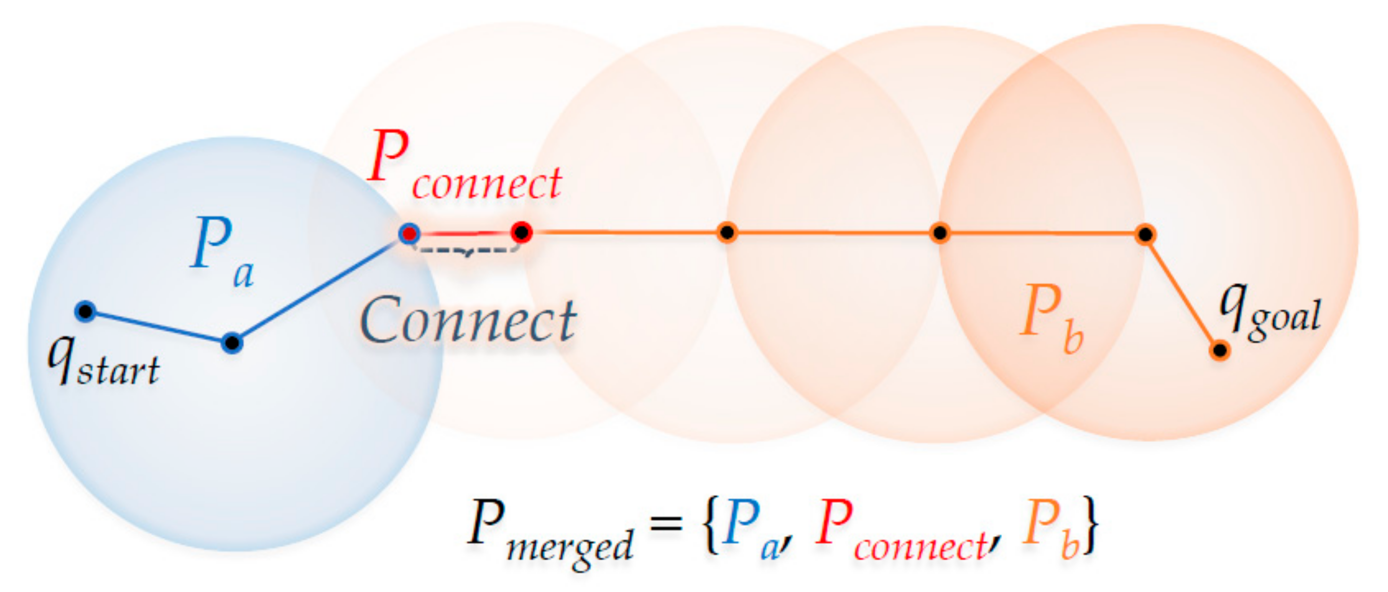
3.3. Pseudocode of the Connect Method from the RRT-Connect Algorithm

This section introduces the ‘Connect’ method used in pseudocode (A1) of the RRT-Connect algorithm in Section 3.1.

Algorithm 3 shows the pseudocode of the ‘Connect’ method in the RRT-Connect algorithm. Here, T_a, T_b, and q_newB are from the ‘Extend’ method (A2).

Algorithm 3 Pseudocode of the Original ‘Connect’ Method from the RRT-Connect Algorithm
Input: Preach ← Path Preach from RRT-Connect Ta ← Tree Ta from RRT-Connect Tb ← Tree Tb from RRT-Connect qnewB ← Position qnewB from RRT-Connect λ ← Step Length λ from RRT-Connect Output: freach ← Result of Boolean freach Preach ← Result of Path Pmerged //Return by Reference Initialize: freach ← False
BeginConnectProcedure fromRRT-Connect
1	IfisInside(qnewA, qnewB, λ) then
2	Pa ← Path from Root Node [qstart] to Last Inserted Node [qnewA] in Ta
3	Pb ← Path from qnewB to Root Node [qgoal] in Tb
4	Pconnect ← Path from Last Inserted Node [qnewA] in Ta to qnewB in Tb
5	Pmerged ← Merge Path Pa to Pb via Pconnect
6	freach ← True
EndConnectProcedure fromRRT-Connect

The tree merging process is as follows: create a path P_a from the root node (q_start) of T_a to the last inserted node (q_newA), and a path P_b from q_newB of T_b to the root node (q_goal). Then, create a path P_connect from q_newB of P_b to the last inserted node (q_newA) of T_a and merge in the order of P_a, P_connect, and P_b, thereby completing planning the path P_merged from q_start to q_goal. After this, it returns True (f_trap), and the ‘Connect’ method ends.

Figure 4 shows the ‘Connect’ method in the RRT-Connect algorithm. If the q_newB of T_b is extended in the direction of the q_newA by the ‘Extend’ method shown in Figure 3, the point where the two trees merge (when q_newB has expanded in the direction of q_newA where T_a enters the λ radius centered at q_newA) with each other is the part marked as ‘Connect’. As a result, the path P_a becomes from the position q_start to the position q_newA in T_a, the path P_connect goes from position q_newA to position q_newB and the path P_b goes from position q_newB to position q_goal in T_b. The merged path P_merged goes from q_start to q_goal.

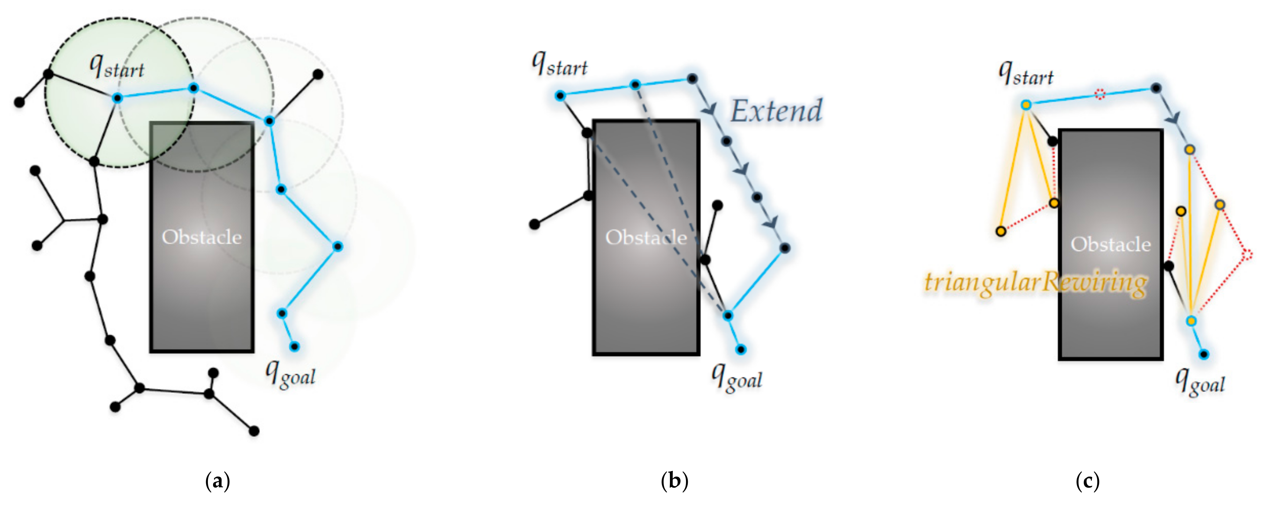
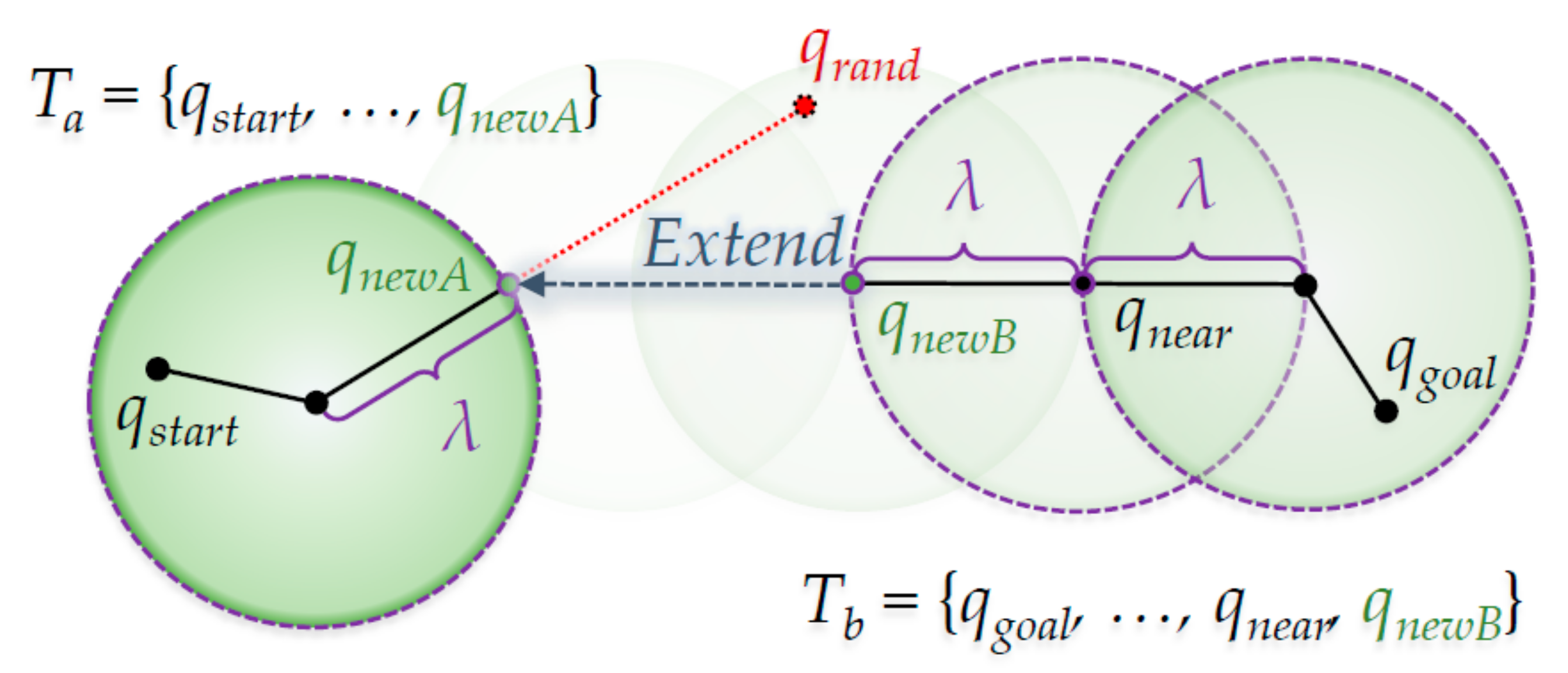
4. Proposed Triangular Inequality-Based RRT-Connect Algorithm

The proposed triangular inequality-based RRT-Connect algorithm is a rewire based on the principle of triangular inequality between nodes on a path planned in the RRT-Connect algorithm, so it is closer to the optimal compared to the RRT-Connect. This is like the RRT*-Smart algorithm [16] and Quick-RRT* [17] algorithms, which shorten their paths using the triangular inequality principle for the RRT algorithm. In this paper, the rewire part based on the triangular inequality principle is called the ‘Triangular-Rewiring’ method.

The proposed triangular inequality-based RRT-Connect algorithm requires the following assumptions:

• There is only one start point and one goal point even though the goal point may be changed incrementally as time goes on.
• The robot is capable of omnidirectional motion.

Therefore, this chapter introduces the proposed ‘Triangular-Rewiring’ method for the RRT-Connect algorithm, and performs mathematical modeling to confirm the validity that the proposed ‘Triangular-Rewiring’ method is always shorter when applied to the RRT-Connect algorithm. After checking through, we will propose how to apply the ‘Triangular-Rewiring’ method to the RRT-Connect algorithm.

The method of applying the RRT-Connect algorithm of the proposed ‘Triangular-Rewiring’ method is proposed when a new node is inserted into the tree in the ‘Extend’ method (A2) and ‘Connect’ method (A3), the main methods of the RRT-Connect algorithm introduced in Chapter 3. It is inserted after rewiring (or after determining) through the ‘Triangular-Rewiring’ method. That is, this chapter introduces the ‘Extend’ and ‘Connect’ methods to which the proposed ‘Triangular-Rewiring’ method is applied.

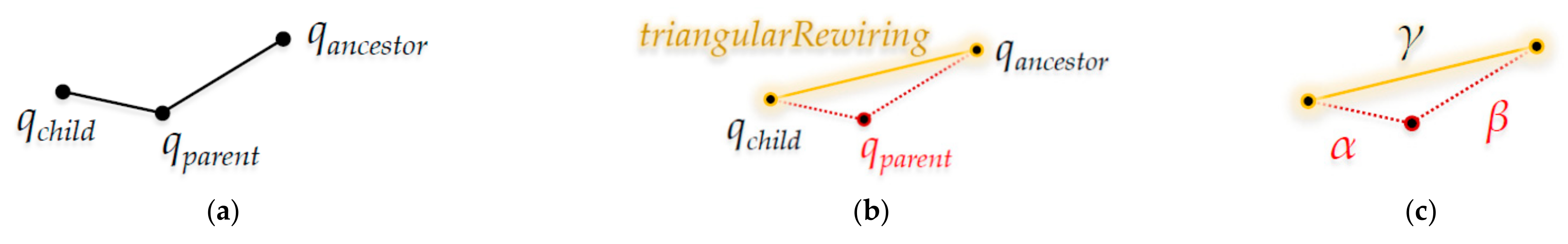
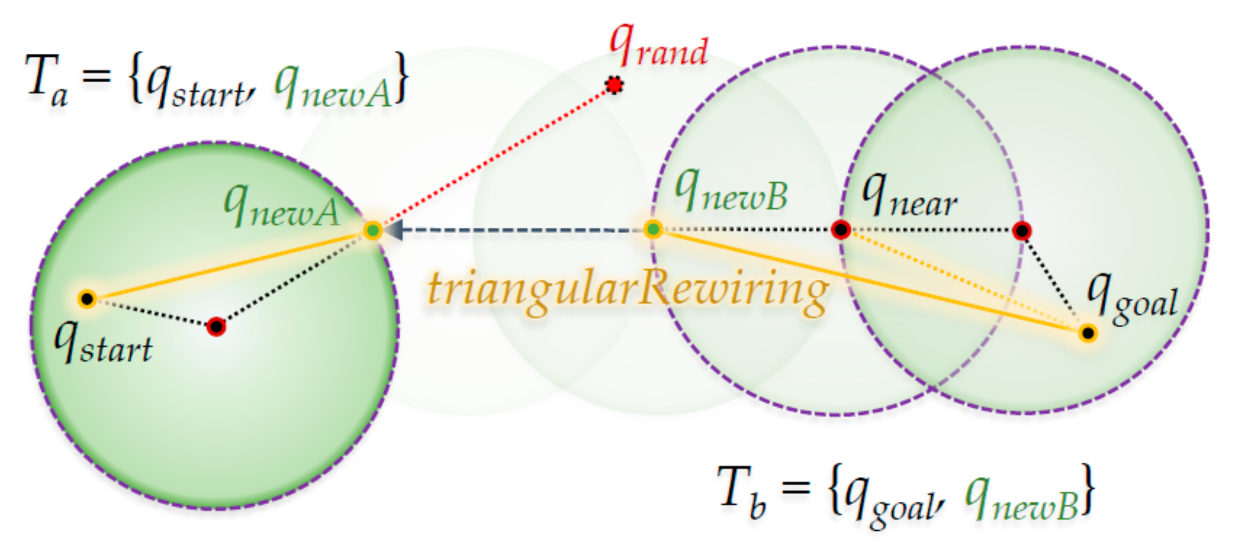
4.1. Pseudocode of the Proposed Triangular-Rewiring Method for the Improved RRT-Connect Algorithm

This section introduces the ‘Triangular-Rewiring’ method for the proposed triangular inequality-based RRT-Connect algorithm.

Algorithm 4 shows the pseudocode of the ‘Triangular-Rewiring’ method applicable in the ‘Extend’ (A2) and ‘Connect’ (A3) methods of the RRT-Connect algorithm. When inserting a new node and edge in T_a or T_b in the ‘Extend’ method (A5), when a tree T_merged (P_merged) in which T_a and T_b trees are merged in the ‘Connect’ method is created (A6), rewiring is performed on the tree T.

Algorithm 4 Pseudocode of the Proposed ‘Triangular-Rewiring’ Method for the RRT-Connect Algorithm
Input: qchild ← Position {qnew/qnewA/qnewB} from {Extend/Connect} qparent ← Position qnear from {Extend/Connect} T ← Tree {Tmerged/Ta/Tb} from {Extend/Connect} C ← Position Set C from {Extend/Connect} Output: {Tmerged/Ta/Tb} ← Result of T
BegintriangularRewiringProcedure fromExtend, Connect
1	qancestor ← Position of Parent Node of qparent in T
2	If NotisTrapped(qancestor, qchild, C) then
3	T ← Delete Node<qparent>, Edge<qparent, qchild> and Edge<qparent, qancestor> from T
4	qparent ← qancestor
5	qancestor ← Position of Parent Node of qancestor in T
6	While Not qancestor = Null do
7	If Not isTrapped(qancestor, qchild, C) then
8	T ← Delete Node<qparent> and Edge<qparent, qancestor> from T
9	qparent ← qancestor
10	qancestor ← Position of Parent Node of qancestor in T
11	Else
12	Break
13	T ← Insert Edge<qparent, qchild> to T
14	Else
15	T ← Insert Node<qchild> and Edge<qchild, qparent> to T
EndtriangularRewiringProcedure fromExtend, Connect

In the ‘Extend’ and ‘Connect’ methods, q_new (or q_newA or q_newB) is inserted as a q_child and q_near is inserted as a candidate for the node’s parent node. From q_parent, the node’s parent node (a second ancestor node candidate based on q_child) is called q_ancestor. Next, it is determined whether an obstacle exists between q_ancestor and q_child (using the isTrapped function). If there is an obstacle (True), the ‘Triangular-Rewiring’ process is skipped and q_child is inserted into the child node of q_parent in T such that the contents of the ‘Extend’ and ‘Connect’ methods from the RRT-Connect algorithm are the same. If there is no obstacle (False), the ‘Triangular-Rewiring’ process proceeds.

The ‘Triangular-Rewiring’ process is as follows: Delete node where position q_parent and the edges between q_child and q_ancestor nodes connected to q_parent. In other words, it disconnects the existing q_parent and q_child and prepares to connect q_child to q_ancestor, the candidate parent node of q_child. Again, q_parent becomes its parent node q_ancestor and q_ancestor becomes the parent node of q_ancestor. Then, as previously done, determine whether an obstacle exists between q_ancestor and q_child (using the isTrapped function). This iterative process continues until no q_ancestor exists (when no parent node exists for the previous q_ancestor, i.e., when q_ancestor is q_start) or an obstacle exists between q_child and q_ancestor. Then, in tree T, the last created q_parent is inserted as the parent node of q_child.

4.2. Mathematical Modeling of the Proposed Triangular Inequality-Based RRT-Connect Algorithm

This section introduces the mathematical modeling of the proposed triangular inequality-based RRT-Connect algorithm. The results show that the proposed algorithm is more efficient in terms of path length than the RRT-Connect algorithm. For reference, this mathematical modeling is based on a two-dimensional Euclidean space.

Equations (1) and (2) define the path length ${\mathrm{𝕕}}_n\left(q_i\right)$ between an arbitrary node q_i and its parent node in the RRT algorithm

$$D\left(q_i, \xi \left(q_i\right)\right)=\sqrt{{\left(\xi \left(q_i\right)·x-q_i·x\right)}^2+{\left(\xi \left(q_i\right)·y-q_i·y\right)}^2},$$

(1)

$$\therefore {\mathrm{𝕕}}_n\left(q_i\right)=D\left({\xi }^n\left(q_i\right),{\xi }^{n+1}\left(q_i\right)\right)$$

(2)

Here, q_i refers to the i-th inserted arbitrary node and takes the x and y coordinate values of the node as an element. The ξ function receives an arbitrary node as a variable and returns the parent node of this node. Equation (1) obtains the distance between an arbitrary node q_i and its parent node, which can be summarized as a function ${\mathrm{𝕕}}_n$ as in Equation (2). Here, n is the distance between the ancestor node and its parent node, based on an arbitrary node. That is, the ξ function to the power of n (n ≥ 0) can be represented as ${\xi }^n\left(q_i\right):=\stackrel{n}{\left(\overbrace{\xi \circ \xi \circ \dots \circ \xi }\right)}\left(q_i\right)$; when n is 0, ${\xi }^0\left(q_i\right):=q_i$ holds.

In addition, consider starting with an arbitrary node q_i and going back to the parent node to find the distance between the n-th ancestor node and the (n + 1)-th ancestor node; this can be represented as $D\left({\xi }^n\left(q_i\right),{\xi }^{n+1}\left(q_i\right)\right)$.

Equations (3) and (4) show the path length ${\mathbb{D}}_R$ from the start position q_start to the goal position q_goal by the RRT algorithm

$${\xi }^{\delta +1}\left(q_{goal}\right)=q_{start},$$

(3)

$$\therefore {\mathbb{D}}_R={\displaystyle \sum }_{n=0}^{\delta }{\mathrm{𝕕}}_n\left(q_{goal}\right)$$

(4)

Equation (3) shows when the (δ + 1)-th ancestor node from q_goal is q_start, where δ is the upper limit of ${\displaystyle \sum }_{n=0}^{\delta }{\mathrm{𝕕}}_n\left(q_{goal}\right)$ for obtaining the path length ${\mathbb{D}}_R$ in Equation (4). In other words, Equation (4) is the sum of the distances from q_goal to the first ancestor node (parent node) of q_goal and the distance from the first ancestor node (parent node) of q_goal to the second ancestor of q_goal, …, and (δ − 1)-th ancestor node to the δ-th ancestor node (q_start).

Figure 5 shows an abstract process of the ‘Triangular-Rewiring’ method. As shown in Figure 5a, if the parent node of q_child is q_parent, the parent node of q_parent is q_ancestor, and q_ancestor is the second ancestor of q_child, this can be represented as Equation (5):

$$q_{ancestor}=\xi \left(q_{parent}\right)={\xi }^2\left(q_{child}\right)$$

(5)

If the distances between the edges connecting each node are the α between q_child and q_parent, the β between q_parent and q_ancestor, and the γ between q_child and q_ancestor is as shown in Figure 5c, this can be represented as Equation (6) using the principle of the triangular inequality

$$\alpha +\beta \ge \gamma$$

(6)

Equations (7) and (8) show the distance relationship between the ancestor nodes of q_child

$$\left(q_{child}, \xi \left(q_{child}\right)\right)=\alpha ,D\left(\xi \left(q_{child}\right), {\xi }^2\left(q_{child}\right)\right)=\beta ,D\left(q_{child}, {\xi }^2\left(q_{child}\right)\right)=\gamma ,$$

(7)

$$\therefore D\left(q_{child}, \xi \left(q_{child}\right)\right)+D\left(\xi \left(q_{child}\right), {\xi }^2\left(q_{child}\right)\right)\ge D\left(q_{child}, {\xi }^2\left(q_{child}\right)\right)$$

(8)

Equation (7) can be summarized as Equation (8) by substituting Equation (5), which represents the relationship between the n-th ancestor nodes of q_child, with the distance as Equation (1) in Equation (6), which represents the distance between each node as a triangular inequality.

Equations (9)–(15) show that the path of the RRT algorithm applying the ‘Triangular-Rewiring’ method is always shorter or equal to that planned by the original RRT algorithm. Equation (9) shows the sequence index k_j to compare the distance $\mathrm{𝕦}$ when applying the ‘Triangular-Rewiring’ method with distance $\mathrm{𝕕}$ when this method is not applied

$$k_j={\tau }_j+{k^{\prime }}_j,{k^{\prime }}_j=\left\{\begin{array}{cc}\hfill 0,& j=0\\ \hfill k_{j-1}+1,& j\ge 1\end{array}\right.$$

(9)

Here, j is a sequence index for $\mathrm{𝕦}$. That is, k_j can be considered a sequence index for $\mathrm{𝕕}$. Currently, ${\tau }_j$ is the number of times that rewiring occurs in the j-th.

If this is summarized by Equation (1) for a distance based on an arbitrary node q_i, it is as Equation (10). For example, as shown in Figure 5, if j is 0 and 1 a rewire occurs (${\tau }_0$ = 1), it can be represented in combination with the distance relationship of Equation (8) for q_child, as in Equation (11)

$${\mathrm{𝕦}}_{k_j}\left(q_i\right)=D\left({\xi }^{{k^{\prime }}_j}\left(q_i\right), {\xi }^{k_j+1}\left(q_i\right)\right),$$

(10)

$${\mathrm{𝕕}}_0\left(q_{child}\right)+{\mathrm{𝕕}}_1\left(q_{child}\right)={\displaystyle \sum }_{n=0}^1{\mathrm{𝕕}}_n\left(q_{child}\right)\ge {\mathrm{𝕦}}_{k_0=1}\left(q_{child}\right)$$

(11)

The result of Equation (11) can be generalized as shown in Equation (12)

$$\therefore {\displaystyle \sum }_{n=0}^{k_j}{\mathrm{𝕕}}_n\left(q_i\right)\ge {\mathrm{𝕦}}_{k_j}\left(q_i\right)$$

(12)

For $\mathrm{𝕕}$ based on an arbitrary node q_i, the path length ${\displaystyle \sum }_{n=j}^{k_j}{\mathrm{𝕕}}_n$ from the j-th to k_j-th arbitrary sequence index is always longer or equal to the distance ${\mathrm{𝕦}}_{k_j}$ of the k_j-th sequence index. That is, in an arbitrary path, it can be confirmed that the distance $\mathrm{𝕦}$ rewired by the ‘Triangular-Rewiring’ method is at least equal (if the distances of $\mathrm{𝕕}$ and $\mathrm{𝕦}$ are the same, the rewired line segments are on a straight line) or always shorter than $\mathrm{𝕕}$ when not rewired.

Figure 6 shows the ‘Triangular-Rewiring’ process for the path from q_start to q_goal based on Equations (5)–(12) (at this time, it is assumed that the node of the path shown in the figure is not positioned in a straight line). As shown in Figure 6b, a total of two rewires occurred (${\tau }_0=2$) between q₀ and q₃ (${\xi }^3\left(q_0\right)$), and a total of one rewire occurred (${\tau }_3=1$) between q₅ (${\xi }^5\left(q_0\right)$) and q₇ (${\xi }^7\left(q_0\right)$). In that case, as shown in Figure 6e, k₀ is 2, k₁ is 3, k₂ is 4, and k₃ is 6 according to Equation (9).

Comparing Figure 6c,e, according to Equation (7), the rewired distance ${\mathrm{𝕦}}_2\left(q_0\right)$ is shorter than the path length ${\displaystyle \sum }_{n=0}^2{\mathrm{𝕕}}_n\left(q_0\right)$ from ${\mathrm{𝕕}}_0$ to ${\mathrm{𝕕}}_2$ and the rewired distance ${\mathrm{𝕦}}_6\left(q_0\right)$ is shorter than the path length ${\displaystyle \sum }_{n=5}^6{\mathrm{𝕕}}_n\left(q_0\right)$ from ${\mathrm{𝕕}}_5$ to ${\mathrm{𝕕}}_6$. That is, when comparing before applying the ‘Triangular-Rewiring’ method in Figure 6a and after applied this method in Figure 6f, the path afterward looks shorter.

Equations (13) and (14) show the path length ${\mathbb{D}}_R$ when the ‘Triangular-Rewiring’ method is not applied and the path length ${\mathbb{U}}_R$ when the method has been applied for an arbitrary path (start position: q_start, goal position: q_goal), as shown in Figure 6

$$k_{\phi }=\delta ,$$

(13)

$${\mathbb{D}}_R={{\displaystyle \sum }}_{n=0}^{\delta }{\mathrm{𝕕}}_n\left(q_{goal}\right)={{\displaystyle \sum }}_{j=0}^{\phi }{{\displaystyle \sum }}_{n={k^{\prime }}_j}^{k_j}{\mathrm{𝕕}}_n\left(q_{goal}\right),{\mathbb{U}}_R={{\displaystyle \sum }}_{j=0}^{\phi }{\mathrm{𝕦}}_{k_j}\left(q_{goal}\right)$$

(14)

Equation (13) shows the upper limit when the index n of d is δ in Equation (3); when this is substituted into the sequence index k_j, if k_j is δ, j becomes φ. In that case, as in Equation (14), ${\mathbb{D}}_R$ is used to compare the ${\displaystyle \sum }_{n=0}^{\delta }{\mathrm{𝕕}}_n\left(q_{goal}\right)$ shown in Equation (4) with ${\mathbb{U}}_R$, reflecting the sequence k_j. It can be represented as ${\displaystyle \sum }_{j=0}^{\phi }{\displaystyle \sum }_{n={k^{\prime }}_j}^{k_j}{\mathrm{𝕕}}_n\left(q_{goal}\right)$, and ${\mathbb{U}}_R$ can be represented as ${\displaystyle \sum }_{j=0}^{\phi }{\mathrm{𝕦}}_{k_j}\left(q_{goal}\right)$.

Equation (15) shows when the equation summarized in Equation (14) is substituted into Equation (12)

$$\therefore {\mathbb{D}}_R\ge {\mathbb{U}}_R$$

(15)

Finally, as can be confirmed using Equation (15), ${\mathbb{U}}_R$ as a result of applying the ‘Triangular-Rewiring’ method to the distance of an arbitrary path (start position: q_start, goal position: q_goal) is at least equal (If the distances of $\mathbb{D}$ and $\mathbb{U}$ are the same, when the rewired line segments are on a straight line) to or always shorter than ${\mathbb{D}}_R$; as a result, this method is not applied.

Equations (16)–(18) show the path length ${\mathbb{D}}_A$ of the path from the start position (root node) of T_a to the last (inserted node) position q_newA and the path length ${\mathbb{U}}_A$ when the ‘Triangular-Rewiring’ method has been applied to the path. In addition, it shows that ${\mathbb{U}}_A$ is at least equal to or always shorter than ${\mathbb{D}}_A$:

$${\xi }^{{\delta }_A+1}\left(q_{newA}\right)=q_{start},k_{{\phi }_A}={\delta }_A,$$

(16)

$${\mathbb{D}}_A={{\displaystyle \sum }}_{j=0}^{{\phi }_A}{{\displaystyle \sum }}_{n={k^{\prime }}_j}^{k_j}{\mathrm{𝕕}}_n\left(q_{newA}\right),{\mathbb{U}}_A={{\displaystyle \sum }}_{j=0}^{{\phi }_A}{\mathrm{𝕦}}_{k_j}\left(q_{newA}\right),$$

(17)

$$\therefore {\mathbb{D}}_A\ge {\mathbb{U}}_A$$

(18)

Equations (19)–(21) show the path length ${\mathbb{D}}_B$ of the path from the start position (root node) of T_b to the last (inserted node) position q_newB and the path length ${\mathbb{U}}_B$ when the ‘Triangular-Rewiring’ method has been applied to the path. In addition, it shows that ${\mathbb{U}}_B$ is at least equal to or always shorter than ${\mathbb{D}}_B$:

$${\xi }^{{\delta }_B+1}\left(q_{newB}\right)=q_{goal},k_{{\phi }_B}={\delta }_B,$$

(19)

$${\mathbb{D}}_B={{\displaystyle \sum }}_{j=0}^{{\phi }_B}{{\displaystyle \sum }}_{n={k^{\prime }}_j}^{k_j}{\mathrm{𝕕}}_n\left(q_{newB}\right),{\mathbb{U}}_B={{\displaystyle \sum }}_{j=0}^{{\phi }_B}{\mathrm{𝕦}}_{k_j}\left(q_{newB}\right),$$

(20)

$$\therefore {\mathbb{D}}_B\ge {\mathbb{U}}_B$$

(21)

Therefore, Equations (16) and (19) can be derived from Equations (3) and (13), Equations (17) and (20) from Equation (14), and Equations (18) and (21) from Equation (15).

As a result, Equations (22) and (23) show that RRT-Connect with the proposed ‘Triangular-Rewiring’ method is at least the same or better in terms of path length than the RRT-Connect algorithm without the method

$${\mathbb{D}}_R={\mathbb{D}}_A+{\mathbb{D}}_B+D\left(q_{newA}, q_{newB}\right),{\mathbb{U}}_R\le {\mathbb{U}}_A+{\mathbb{U}}_B+D\left(q_{newA}, q_{newB}\right),$$

(22)

$$\therefore {\mathbb{D}}_R\ge {\mathbb{D}}_A+{\mathbb{D}}_B\ge {\mathbb{U}}_A+{\mathbb{U}}_B\ge {\mathbb{U}}_R$$

(23)

${\mathbb{D}}_R$ (Equation (4)), which refers to the path length of the RRT-Connect algorithm path without the ‘Triangular-Rewiring’ method, is represented by the sum of the distance ${\mathbb{D}}_A$ of the partial path P_a (Equation (17)), the distance ${\mathbb{D}}_B$ of the partial path P_b (Equation (20)), and the distance $D\left(q_{newA}, q_{newB}\right)$ between q_newA and q_newB as shown in Equation (22).

${\mathbb{U}}_R$ (Equation (14)), which refers to the path length of the RRT-Connect algorithm path with the ‘Triangular-Rewiring’ method, is equal to or shorter than the sum of the distance ${\mathbb{U}}_A$ of the partial path P_a for the RRT-Connect (Equation (17)), the distance ${\mathbb{U}}_B$ of the partial path P_b (Equation (20)), and the distance $D\left(q_{newA}, q_{newB}\right)$ between q_newA and q_newB as shown in Equation (22).

Here, Equation (23) shows that ${\mathbb{U}}_R$ is at least equal to or shorter than ${\mathbb{D}}_R$ in the RRT algorithm summarized in Equation (15), and it is used efficiently in the RRT-Connect algorithm.

4.3. Pseudocode of Proposed Extend Method for the Improved RRT-Connect Algorithm

This section introduces the ‘Extend’ method in the proposed triangular inequality-based RRT-Connect algorithm. This proposed ‘Extend’ method (A5) replaces the ‘Extend’ method (A3) in the pseudocode of the RRT-Connect algorithm (A2).

Algorithm 5 is the application of the ‘Triangular-Rewiring’ method (A4) to the original ‘Extend’ method (A2) of the RRT-Connect algorithm. Compared to the original ‘Extend’ method, the part where a node is newly inserted in the tree in lines 9 and 16 is inserted through the ‘Triangular-Rewiring’ method. Other than that, the contents are the same as the original ‘Extend’ method.

Algorithm 5 Pseudocode of the Proposed ‘Extend’ Method for the RRT-Connect Algorithm
Input: Ta ← Tree Ta from RRT-Connect Tb ← Tree Tb from RRT-Connect qnewB ← Position qnewB from RRT-Connect qrand ← Position qrand from RRT-Connect λ ← Step Length λ from RRT-Connect C ← Position Set C from RRT-Connect Output: ftrap ← Result of Boolean ftrap Ta ← Result of Tree Ta //Return by Reference Tb ← Result of Tree Tb //Return by Reference qnewB ← Result of Position qnewB //Return by Reference Initialize: ftrap ← False
BeginExtendProcedure fromRRT-Connect
1	qnear ← Find Position of Nearest Node in Ta from qrand
2	If NotisInside(qnear, qrand, λ) then
3	qnewA ← Position of Intersection Point between Line Segment connecting qrand and qnear, and Circle with Radius λ centered at qnear //2D: Circle, 3D: Sphere, …
4	Else
5	qnewA ← qrand
6	IfisTrapped(qnewA, qnear, C) then
7	ftrap ← True
8	Else
9	Ta ← triangularRewiring(qnewA, qnear, Ta, C)
10	qnear ← Find Position of Nearest Node in Tb from qnewA
11	If isInside(qnear, qnewA, λ) then
12	qnewB ← qnear
13	Else
14	qnewB ← Position of Intersection Point between Line Segment connecting qnewA and qnear, and Circle with Radius λ centered at qnear //2D: Circle, 3D: Sphere, …
15	While Not isTrapped(qnewB, qnear, C) do
16	Tb ← triangularRewiring(qnewB, qnear, Tb, C)
17	If Not isInside(qnewA, qnewB, λ) then
18	qnear ← qnewB
19	qnewB ← Position of Intersection Point between Line Segment connecting qnewA and qnear, and Circle with Radius λ centered at qnear //2D: Circle, 3D: Sphere, …
20	Else
21	Break
EndExtendProcedure fromRRT-Connect

Figure 7 shows the application of the ‘Triangular-Rewiring’ method to Figure 3, which shows the ‘Extend’ method of the RRT-Connect algorithm. In T_a, q_newA and q_start are rewired and q_near and q_goal, and q_newB and q_goal are rewired sequentially in the process of extending from T_b to T_a.

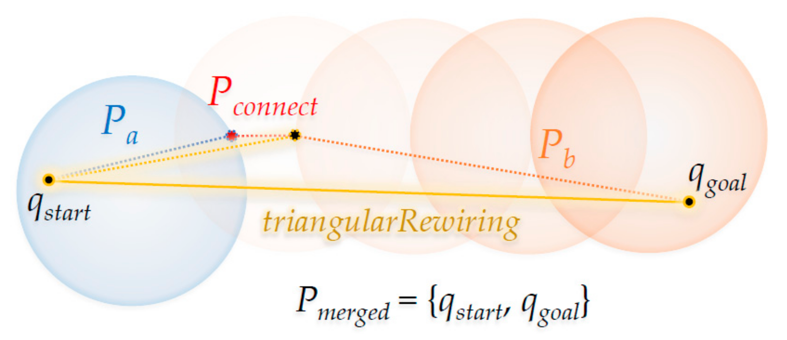
4.4. Pseudocode of the Proposed Connect Method for the RRT-Connect Algorithm

This section introduces the ‘Connect’ method in the proposed triangular inequality-based RRT-Connect algorithm. This proposed ‘Connect’ method (A6) replaces the ‘Connect’ method (A4) in the pseudocode of the RRT-Connect algorithm (A2).

Algorithm 6 is an application of the ‘Triangular-Rewiring’ method (A4) to the ‘Connect’ method (A3) of the RRT-Connect algorithm. Compared to the original ‘Connect’ method, it has been changed to apply the method to the merged tree by considering the ‘Triangular-Rewiring’ method when merging the path, which is in lines 5–10. Other than that, the contents are the same as the original ‘Connect’ method.

Algorithm 6 Pseudocode of the Proposed ‘Connect’ Method for the RRT-Connect Algorithm
Input: Preach ← Path Preach from RRT-Connect Ta ← Tree Ta from RRT-Connect Tb ← Tree Tb from RRT-Connect qnewB ← Position qnewB from RRT-Connect λ ← Step Length λ from RRT-Connect Output: freach ← Result of Boolean freach Preach ← Result of Path Pmerged //Return by Reference Initialize: freach ← False
BeginConnectProcedure fromRRT-Connect
1	IfisInside(qnewA, qnewB, λ) then
2	Pa ← Path from Root Node [qstart] to Last Inserted Node [qnewA] in Ta
3	Pb ← Path from qnewB to Root Node [qgoal] in Tb
4	Pconnect ← Path from Last Inserted Node [qnewA] in Ta to qnewB in Tb
5	Tmerged ← Tree Structure with Merge Path Pa to Pb via Pconnect //1st Insert: qstart, …, n-th Insert: qnewA, (n + 1)-th Insert: qnewB, …, Last Insert: qgoal to Tmerged
6	For i ← Inserted Index of qnewA in Tmerged to (Number of Node in Tmerged) – 1 do
7	qnew ← (i – 1)-th Inserted Node in Tmerged
8	qnear ← i-th Inserted Node in Tmerged
9	Tmerged ← triangularRewiring(qnew, qnear, Tmerged, C)
10	Pmerged ← Path from Root Node [qstart] to Last Inserted Node [qgoal] in Tmerged
11	freach ← True
EndConnectProcedure fromRRT-Connect

When paths P_a and P_b merge in a tree structure of line 5, nodes on the path are inserted in the order of P_a, P_connect, and P_b in the merged tree T_merged. That is, in T_merged, the root node becomes q_start, and when the n-th inserted node at a certain point is q_newA, which is the last inserted node of T_a, the (n + 1)-th inserted node becomes q_newB, which is the last inserted node of T_b. In addition, the last inserted node of T_merged becomes q_goal.

Then, the ‘Triangular-Rewiring’ method is applied to this T_merged. Since it is applied to the tree itself, it determines whether rewiring is possible for all nodes inserted in the tree, and rewires and updates the tree if possible. However, since each node from T_a to T_b is inserted into T_merged, it is not necessary to rewire T_a for which the ‘Triangular-Rewiring’ process has already been performed. Therefore, the ‘Triangular-Rewiring’ process proceeds in the direction of T_b from the q_newA sequence inserted in T_merged. Here, if q_newA is the i-th inserted node, the first node pair to be determined is the (i − 1)-th node q_new (as q_child) and i-th node q_near (as q_parent). When all nodes inserted in T_merged have been determined, the tree structure T_merged is converted into the path P_merged and the method terminates (True).

Figure 8 shows the ‘Triangular-Rewiring’ method applied to Figure 4, which shows the ‘Connect’ method of the RRT-Connect algorithm. When the paths P_a and P_b created from the trees T_a and T_b are merged and the ‘Triangular-Rewiring’ method has been applied (assuming there is no obstacle between q_start and q_goal), the result is P_merged in which q_start and q_goal are connected with a straight line.

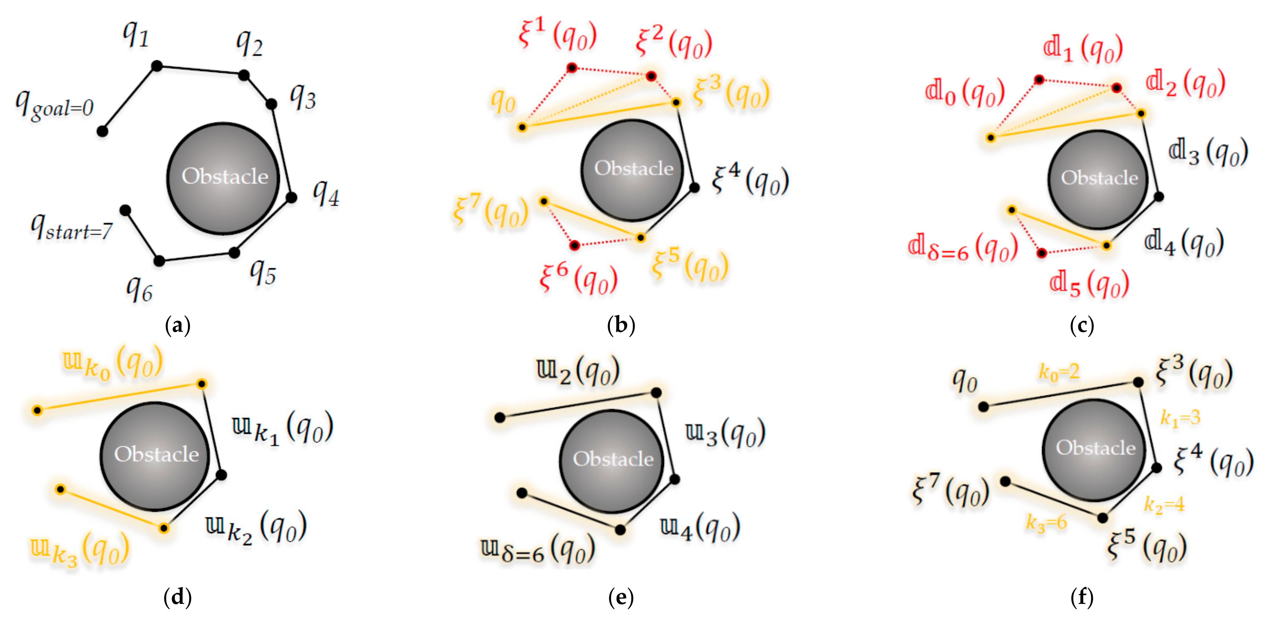
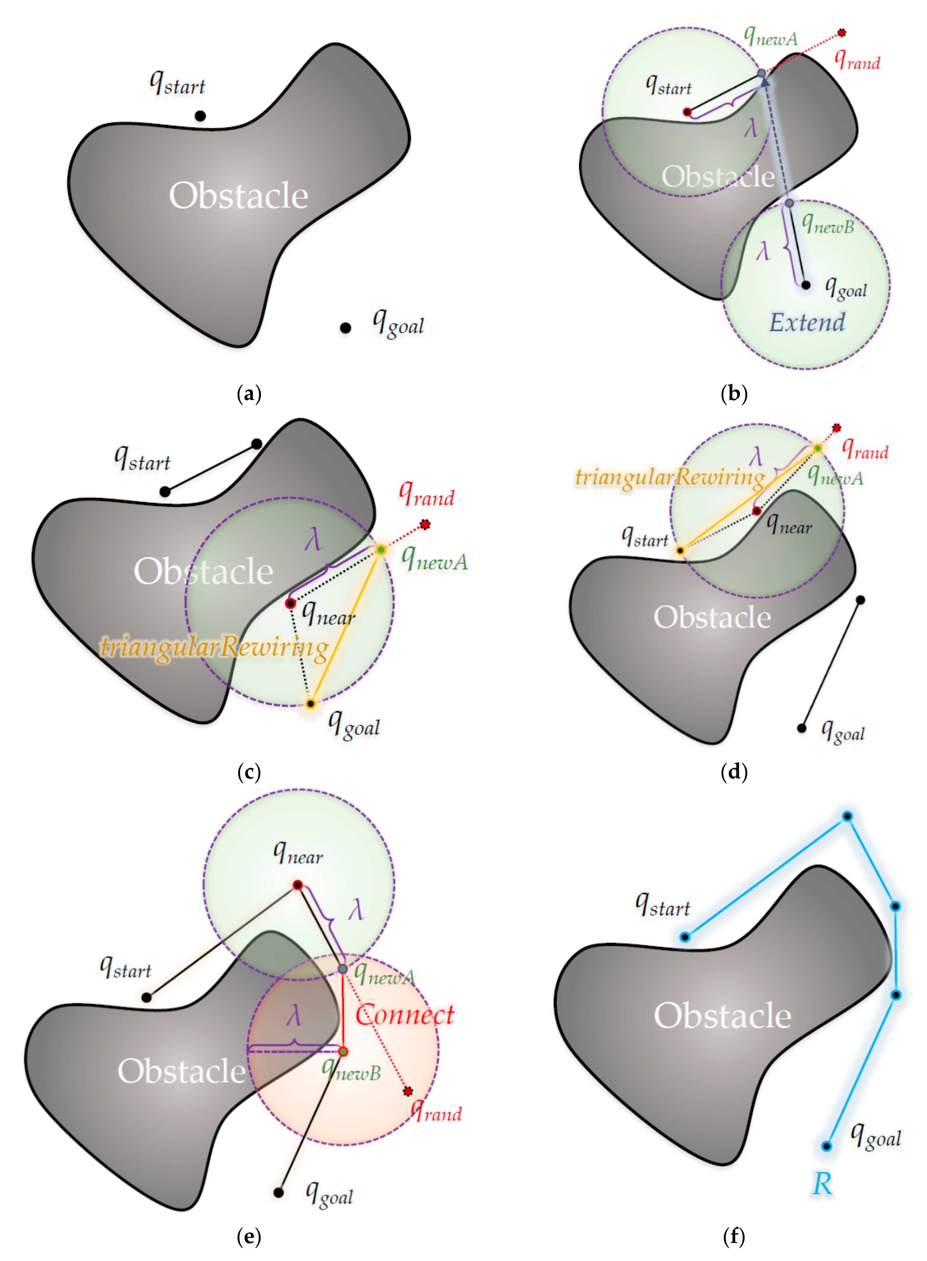
4.5. Process of the Proposed Triangular Inequality-Based RRT-Connect Algorithm

Figure 9 in this section shows the path-planning process of the proposed algorithm by applying the ‘Triangular-Rewiring’ method to the ‘Extend’ and ‘Connect’ methods of the RRT-Connect algorithm.

Figure 9 shows planning a path from the start position q_start to the goal position q_goal through the proposed algorithm, as shown in Figure 9a.

In Figure 9b, the first random sample is generated at position q_rand and q_newA is created at a position separated by the length of λ from q_start in the direction of the position, and q_newA is extended once by the length of λ in the direction of q_newA from q_goal. At this time, since there is no intermediate node between q_newA and q_start, the ‘Triangular-Rewiring’ process is skipped.

In Figure 9c, a second random sample is generated at the q_rand position, and in the direction of the position, q_newA is updated at a location separated by λ length from the nearest node q_near in the tree and rewired between q_newA and q_goal. In this case, since the tree on the opposite side collides with an obstacle to extend in the q_newA direction, the ‘Extend’ process is skipped. In addition, it is assumed that Swap occurs between T_a with initial q_start as the root node and T_b with initial q_goal as the root node between each figure.

In Figure 9d, as shown in Figure 9c, a third random sample is created at the q_rand position and at a position separated by the length of λ in the position direction, at the node q_near that is nearest among nodes in the tree in the position direction, It shows updating q_newA to a position that is the length of λ and rewires it between q_newA and q_start. Here, since it also collides with an obstacle to extend in the direction of q_newA from the tree on the opposite side, the ‘Extend’ process is skipped.

In Figure 9e, the fifth random sample is generated at the q_rand position and q_newA is located at a position separated by the length of λ in the direction of the position, and q_newA is also at a position separated by the length of λ from the nearest node q_near among nodes in the tree toward the position. It is shown when updating that q_newA merges into one tree through the ‘Connect’ process because q_newA is within range of the center of q_newB and the radius of λ. It is assumed that the fourth random sample between Figure 9d,e is generated inside the obstacle, so the q_newA generation process is skipped. Figure 9f shows the result of path R created as a merged tree by ‘Connect’ as shown in Figure 9e.

5. Experimental Results

To verify the performance of the proposed triangular inequality-based RRT-Connect algorithm in this paper, the RRT algorithm, the RRT-Connect algorithm, and the proposed algorithm are compared in various environment maps shown in the experimental environment through the simulator.

Each algorithm was implemented based on the pseudocode (A1–9) shown Section 3 and Section 4 (For the RRT algorithm, refer to the pseudocode (AA1) in Appendix A), and the performance measures used for comparison of various algorithms are Number of samples (samples), Path length (pixels), and Planning time (milliseconds). Each performance measure is experimented with 50 trials from the same start point to the same goal point until the first path has been found). Among the performance measures, as the number of samples decreases, the cost of recalculation in a dynamic environment also decreases, and the path length is a measure of the optimality of the path-planning algorithm. In addition, the Step length (λ) is 30 pixels.

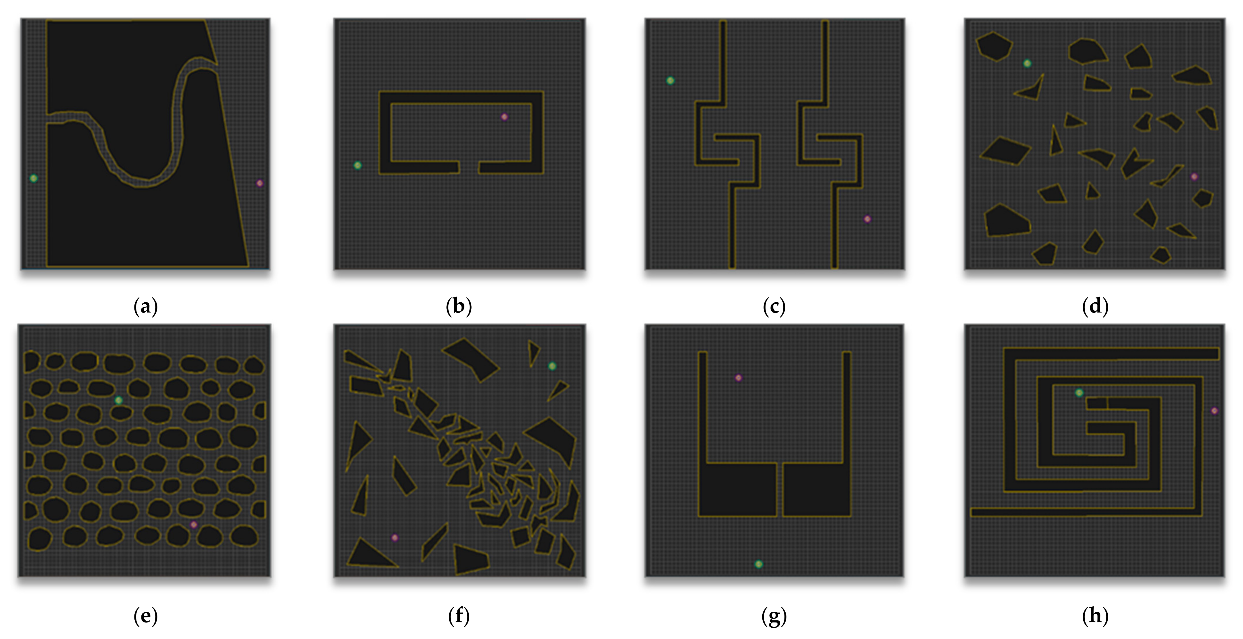
5.1. Experimental Environment

This section introduces the environment map used in the simulation and the simulator used in the simulation with the computer’s performance.

Figure 10 shows the eight environmental maps used in this experiment. The green circle (S) indicates the start point, the purple circle (G) indicates the goal point, and the black polygon on the yellow (blue in the analysis of the experimental results) border indicates to the obstacle. All maps are 600 (horizontal) * 600 (vertical) pixels.

Many environmental maps were considered and used to verify the performance of various path-planning algorithms including the RRT algorithm, [23,24,25,26]. Which environment map to use is important because the expected performance measure varies depending on the obstacles’ placement and shape among other properties.

In this paper, to check the proposed algorithm’s performance, the eight maps shown in Figure 10 were benchmarked in the experimental environment of the paper [27] proposed by Jihee Han in 2017, and each map is expected to have the following features:

Map 1 in Figure 10a seems to be an environment in which it is easy to verify the completeness of the path-planning algorithm. Map 2 in Figure 10b seems to be an environment in which it is also easy to verify the completeness of the path-planning algorithm, and the environment is mainly used to show the solution for the Local Minima problem [28] in the artificial potential field algorithm [26]. Map 3 in Figure 10c seems to be an environment in which it is easy to verify the optimality and completeness of the path-planning algorithm and is an environment that is unfavorable to random sampling path-planning algorithms such as the RRT algorithm. Map 4 in Figure 10d seems to be an environment in which it is easy to verify the optimality and the planning time for the path-planning algorithm, and the cell decomposition algorithm, which increases the computation cost as the angle of obstacle increases, is an unfavorable environment [29]. Map 5 in Figure 10e seems to be an environment in which it is also easy to verify the optimality and planning time of the path-planning algorithm; for the same reason as Map 4, the cell decomposition algorithm is an unfavorable environment. Map 6 in Figure 10f seems to be an environment in which it is easy to verify the optimality, completeness, and planning time of the path-planning algorithm, and it is an environment for comprehensively evaluating the performance. Map 7 in Figure 10g seems to be an environment in which it is easy to verify the completeness and optimality of the path-planning algorithm, and for the same reason as Map 2, it is the environment used in the Artificial Potential Field algorithm. Lastly, Map 8 in Figure 10h seems to be an environment in which it is easy to verify the completeness and planning time of the path-planning algorithm and yet is unfavorable to random sampling path-planning algorithms such as the RRT algorithm.

Since random sampling path-planning algorithms such as the RRT algorithm rely on probabilistic completeness, the number of samples and the planning time are significantly increased as long as there are narrow or fewer entrances for directions to the goal.

Table 1. Computer performance for simulation.

H/W	Specification
CPU	Intel Core i7-6700k 4.00 GHz (8 CPUs)
RAM	32,768 MB (32 GB DDR4)
VGA	Nvidia GeForce GTX 1080 (VRAM 8 GB) SLI (x2)

shows the specifications of the computer used in the simulation. The simulator was developed in C# language (Microsoft Visual Studio Community 2019 version 16.1.6; Microsoft. NET Framework version 4.8.03752), and except for the visual part, only a single thread was used for the calculation. Differences in planning time may occur depending on the computer’s performance capability.

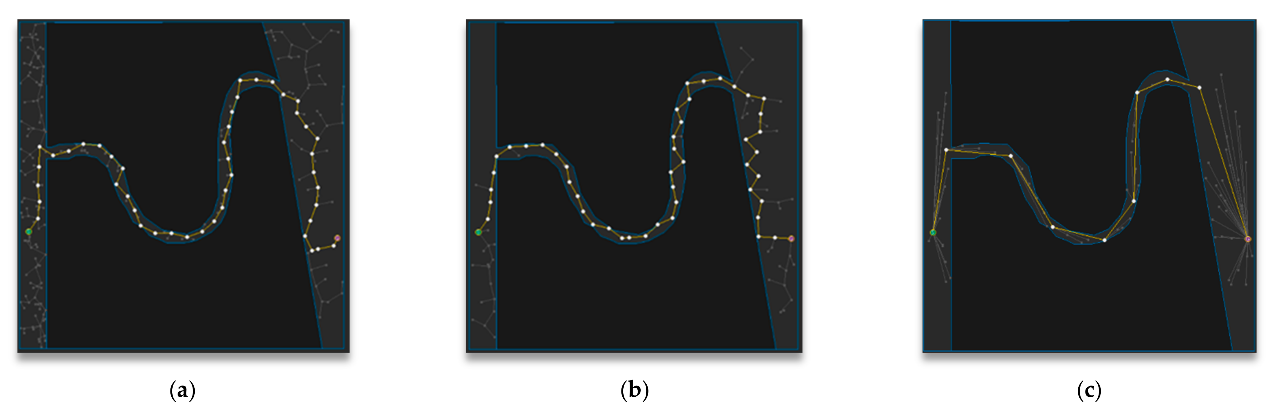
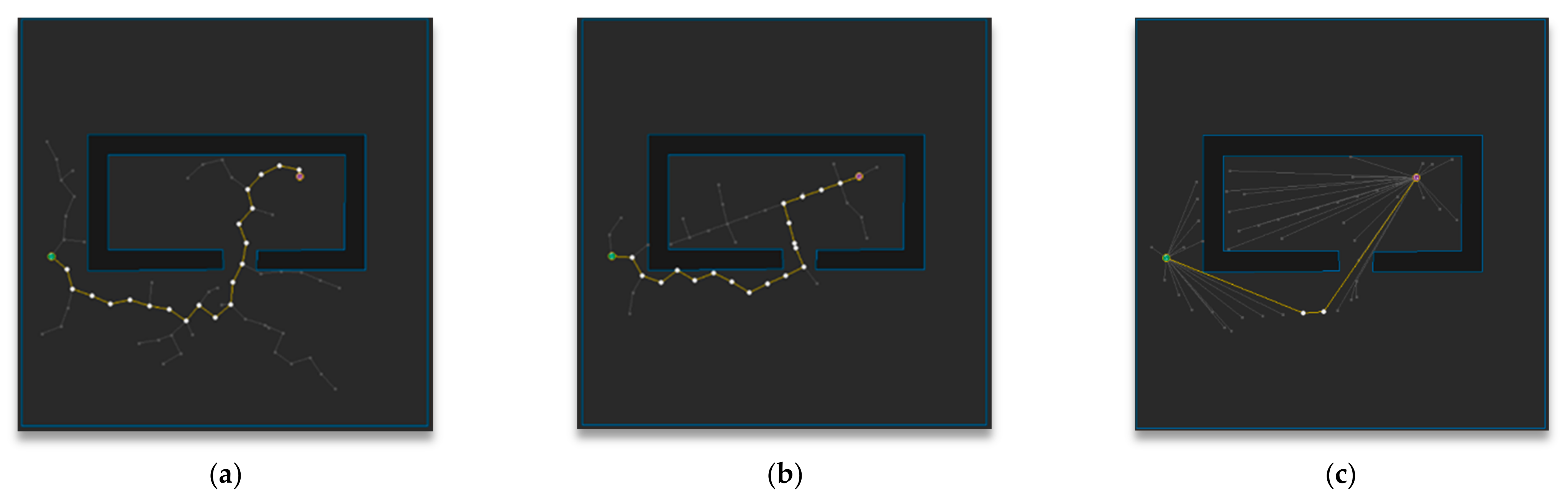
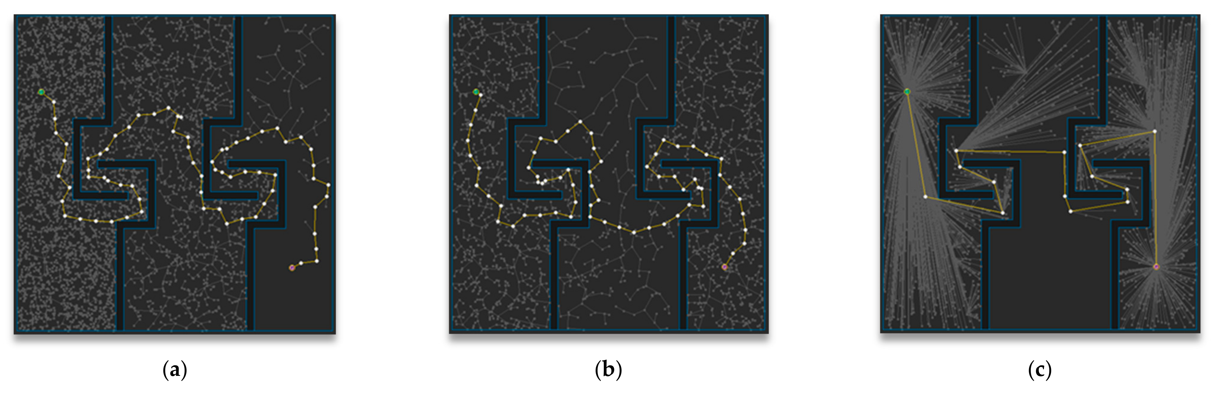
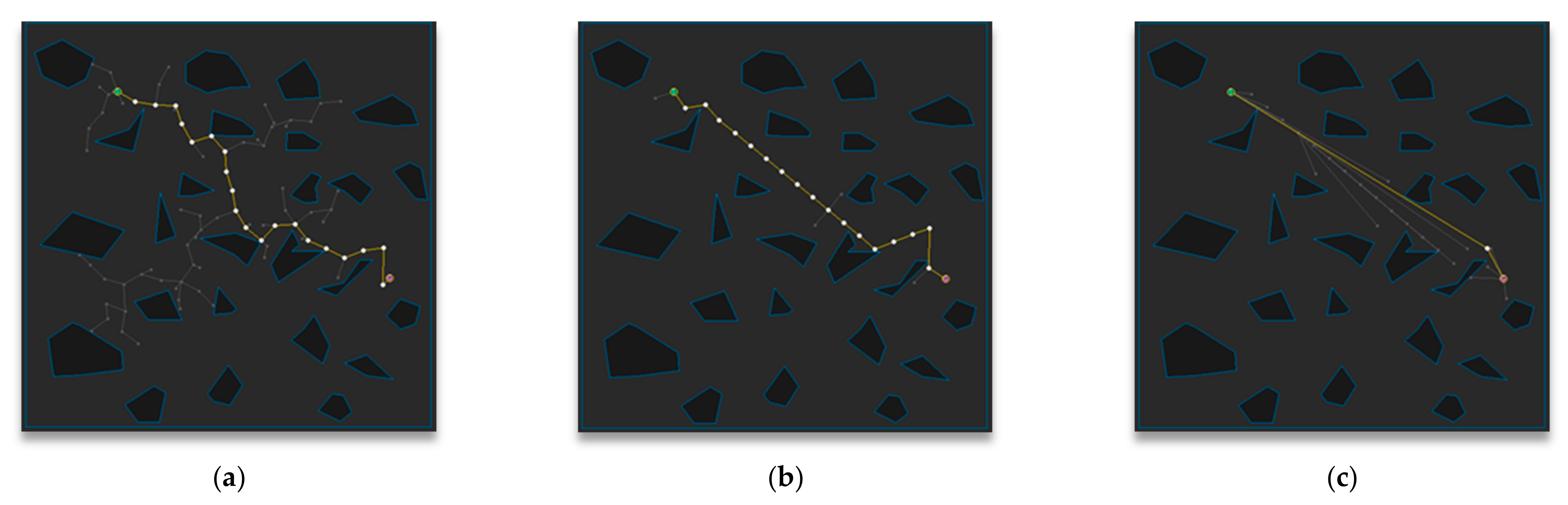
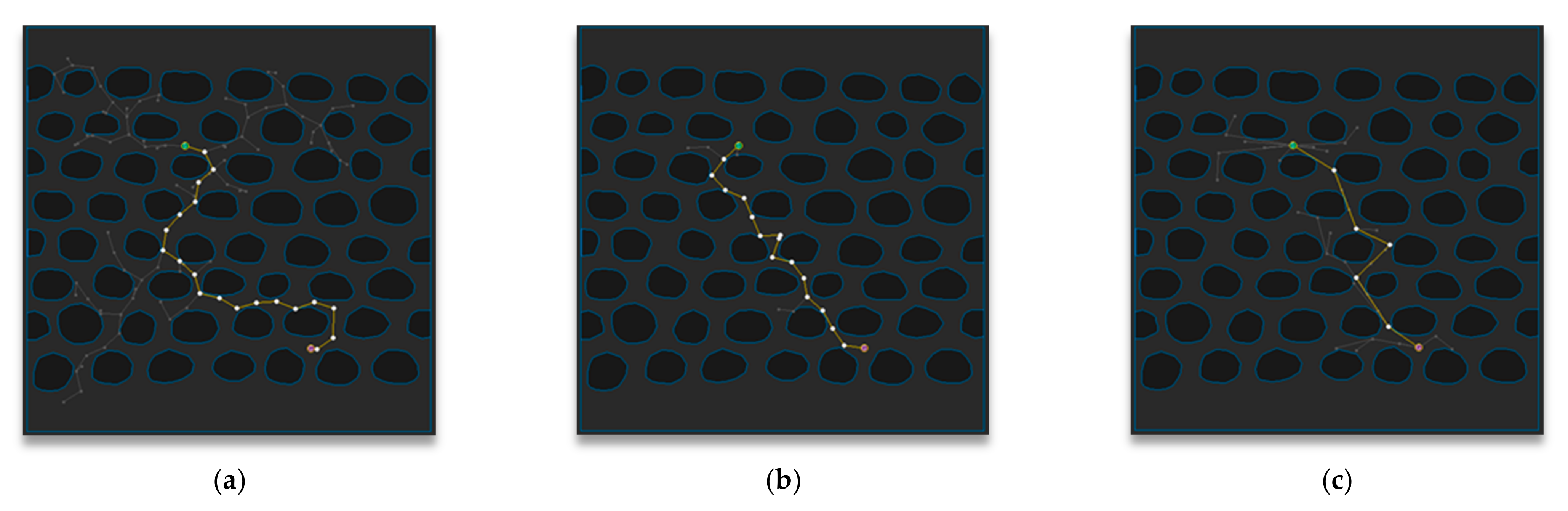
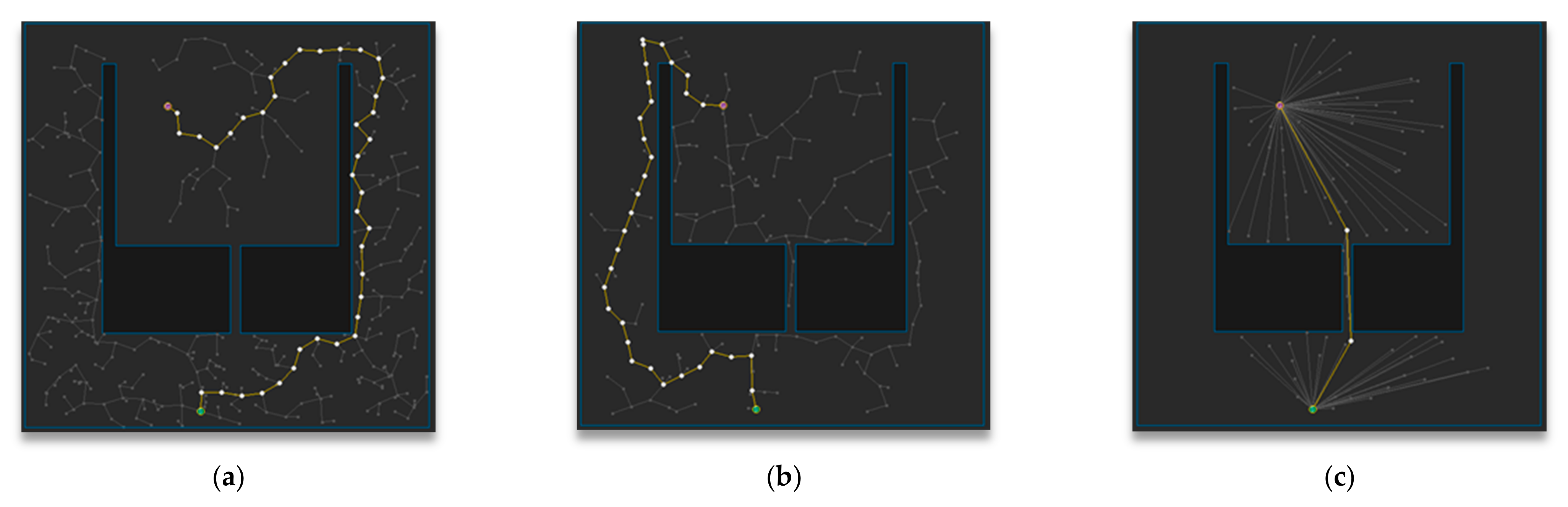
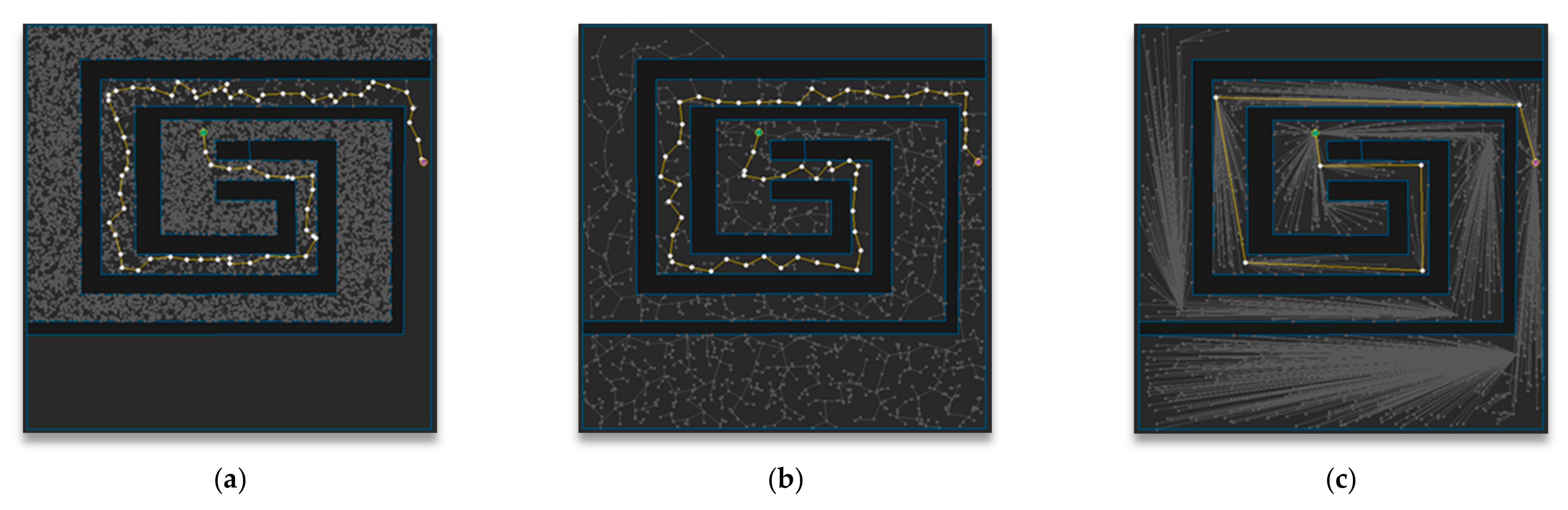
5.2. Experimental Results and Analysis for Each Map

This section checks the experimental results (on average, the number of samples, path length, and planning time) of each algorithm: RRT, RRT-Connect, the proposed algorithm in the eight environment maps (Figure 10) presented in the experimental environment. Each map shows a figure of the path-planning result (of one trial) for each algorithm (Figures 11–18) and the experimental results for the performance measure are shown numerically in a table (Tables 2–9). The figure for each algorithm is for one trial rather than the average of repeated trials and it may differ from the performance measure both visually and by the average numerical performance measure of the repeated trials shown in the table. In particular, the number of samples differs greatly.

The values shown in Tables 2–9 can be expressed as Equations (24) and (25) as

$$A_{cmp}\left(i\right) ={\displaystyle \sum }_{k=0}^T{a}_{cmp{}_k}\left(i\right)/T$$

(24)

Here, $A_{cmp}\left(i\right)$ refers to the performance value of each algorithm shown in Tables 2–9, cmp is the algorithm to be compared, i is the index of the environment map (X-axis in Figures 19, 20 and 21b, k is the repeat index, and T is the number of repeats ($a_{cmp}{}_k\left(i\right)$ is the value of the performance measure a for the k-th implementation of the cmp algorithm in Map i). Fifty repetitions are performed for the experiment in this paper. That is, Equation A shows the average value of the performance when it is repeated T times to check the performance of a certain algorithm in Map i,

$$\therefore x_{cmp}\left(i\right) =A_{cmp}\left(i\right)/A_{RRT}\left(i\right)$$

(25)

Here, $x_{cmp}\left(i\right)$ refers to the Y-axis in Figures 19, 20 and 21a and A is the value of the corresponding performance measure of the algorithm to be compared ($A_{RRT}$ is the value of the RRT algorithm).

In each path-planning result figure, the white circles indicate nodes on the path and the yellow line segments indicate edges between nodes. The gray circles and segments are paths (trees) that have been excluded during path planning. In each path-planning result table, based on 100% of the RRT algorithm for each performance measure, the difference is indicated along with the value of the corresponding performance measure unit.

Figure 11 shows the path-planning results of Map 1 among the environmental maps for each algorithm. Visually, the number of samples looks similar to the RRT-Connect algorithm in Figure 11b and the proposed algorithm in Figure 11c is comparable to the RRT algorithm in Figure 11a, and the path length looks similar for all three algorithms.

Table 2. Experimental result of Map 1 (the parentheses to the right of each value are relative ratios based on RRT 100% ($x_{cmp}\left(1\right)$)).

$\mathit{Performance} \left({\mathit{A}}_{\mathit{c}\mathit{m}\mathit{p}}\left(1\right)\right)$	RRT	RRT-Connect	Proposed Algorithm
Avg. num. of samples (samples)	1216 (100)	729 (60)	823 (68)
Avg. path length (px)	1341 (100)	1343 (100)	1200 (89)
Avg. planning time (ms)	12 (100)	7 (58)	10 (83)

shows the path-planning results (after repeating the trial 50 times) in Map 1 for each algorithm. The average number of samples is the smallest in RRT-Connect algorithm at 60%, and the proposed algorithm is 68% compared to the RRT algorithm, which is 8% less efficient than the RRT algorithm compared to the RRT-Connect algorithm. The average path length is shortest for the proposed algorithm at 89% compared to the RRT algorithm, with little difference in the RRT-Connect algorithm at 100%, and 11% less efficient than the proposed algorithm. The average planning time is the shortest for the RRT-Connect algorithm at 58% compared to the RRT algorithm, and the proposed algorithm is 83% compared to the RRT algorithm, i.e., 15% less efficient than the RRT algorithm.

Figure 12 shows the path-planning results of Map 2 among the environmental maps for each algorithm. Visually, the number of samples looks similar for the RRT-Connect algorithm in Figure 12b and the proposed algorithm in Figure 12c compared to the RRT algorithm in Figure 12a, and the path length looks shortest for the proposed algorithm.

Table 3. Experimental result of Map 2 (the parentheses to the right of each value are the relative ratios based on RRT 100% ($x_{cmp}\left(2\right)$)).

$\mathit{Performance} \left({\mathit{A}}_{\mathit{c}\mathit{m}\mathit{p}}\left(2\right)\right)$	RRT	RRT-Connect	Proposed Algorithm
Avg. num. of samples (samples)	271 (100)	101 (37)	113 (42)
Avg. path length (px)	598 (100)	613 (98)	484 (81)
Avg. planning time (ms)	6 (100)	3 (50)	3 (50)

shows the path-planning result (after repeating the trials 50 times) in Map 2 for each algorithm. The average number of samples is smallest in the RRT-Connect algorithm at 37%, and the proposed algorithm is 42% compared to the RRT algorithm, which is 5% less efficient than RRT algorithm compared to the RRT-Connect algorithm. The average path length of the proposed algorithm is the shortest at 81% compared to the RRT algorithm, while the RRT-Connect algorithm is 98%, which is 17% less efficient than the RRT algorithm compared to the proposed algorithm. The average planning time for the proposed algorithm and the RRT-Connect shows the same performance as the RRT algorithm.

Figure 13 shows the path planning results of Map 3 among the environmental maps for each algorithm. Visually, the number of samples looks similar for the RRT-Connect algorithm in Figure 13b and the proposed algorithm in Figure 13c compared to the RRT algorithm in Figure 13a, and the path length looks shortest for the proposed algorithm.

Table 4. Experimental result of Map 3 (the parentheses to the right of each value are the relative ratios based on RRT 100% ($x_{cmp}\left(3\right)$)).

$\mathit{Performance} \left({\mathit{A}}_{\mathit{c}\mathit{m}\mathit{p}}\left(3\right)\right)$	RRT	RRT-Connect	Proposed Algorithm
Avg. num. of samples (samples)	6106 (100)	4574 (75)	4679 (77)
Avg. path length (px)	1934 (100)	1871 (97)	1489 (77)
Avg. planning time (ms)	866 (100)	299 (35)	313 (36)

shows the result (after repeating the trial 50 times) of path planning in Map 3 for each algorithm. The average number of samples is smallest in the RRT-Connect algorithm at 75%, and the proposed algorithm is 77% compared to the RRT algorithm, which is 2% less efficient than the RRT algorithm compared to the RRT-Connect algorithm. The average path length of the proposed algorithm is the shortest at 77% compared to the RRT algorithm and the RRT-Connect algorithm is 97%, which is 20% less efficient than the RRT algorithm compared to the proposed algorithm. The average planning time is smallest for the RRT-Connect algorithm at 35%, and the proposed algorithm is 36% compared to the RRT algorithm, which is 1% less efficient than the RRT algorithm compared to the RRT-Connect algorithm.

Figure 14 shows the path planning results of Map 4 among the environmental maps for each algorithm. Visually, the number of samples looks smallest for the RRT-Connect algorithm in Figure 14b compared to the others and the path length looks shortest for the proposed algorithm in Figure 14c.

Table 5. Experimental result of Map 4 (The parentheses to the right of each value are relative ratios based on RRT 100% ($x_{cmp}\left(4\right)$)).

$\mathit{Performance} \left({\mathit{A}}_{\mathit{c}\mathit{m}\mathit{p}}\left(4\right)\right)$	RRT	RRT-Connect	Proposed Algorithm
Avg. num. of samples (samples)	290 (100)	28 (10)	32 (11)
Avg. path length (px)	711 (100)	588 (83)	534 (75)
Avg. planning time (ms)	3 (100)	3 (100)	4 (133)

shows the result (after repeating the trial 50 times) of path planning in Map 4 for each algorithm. The average number of samples is smallest in the RRT-Connect algorithm at 10%, and the proposed algorithm is 11% compared to the RRT algorithm, which is 1% less efficient than the RRT algorithm compared to the RRT-Connect algorithm. The average path length of the proposed algorithm is the shortest at 75% compared to the RRT algorithm and the RRT-Connect algorithm is 83%, which is 8% less efficient than the RRT algorithm compared to the proposed algorithm. The average planning time is not different by 100% compared to the RRT algorithm, and the proposed algorithm is 133% compared to the RRT algorithm, i.e., 33% less efficient than the others.

Figure 15 shows the path planning results of Map 5 among the environmental maps for each algorithm. Visually, the number of samples looks similar for the RRT-Connect algorithm in Figure 15b and the proposed algorithm in Figure 15c compared to the RRT algorithm in Figure 15a, and the path length looks similar for the RRT-Connect algorithm and the proposed algorithm.

Table 6. Experimental result of Map 5 (the parentheses to the right of each value are the relative ratios based on RRT 100% ($x_{cmp}\left(5\right)$)).

$\mathit{Performance} \left({\mathit{A}}_{\mathit{c}\mathit{m}\mathit{p}}\left(5\right)\right)$	RRT	RRT-Connect	Proposed Algorithm
Avg. num. of samples (samples)	371 (100)	68 (18)	74 (20)
Avg. path length (px)	554 (100)	588 (106)	465 (84)
Avg. planning time (ms)	13 (100)	2 (15)	2 (15)

shows the results (after repeating the trial 50 times) of path planning in Map 5 for each algorithm. The average number of samples is smallest in RRT-Connect algorithm at 18%, and the proposed algorithm is 20% compared to the RRT algorithm, which is 9% less efficient than the RRT algorithm compared to the RRT-Connect algorithm. The average path length of the proposed algorithm is the shortest at 84% compared to the RRT algorithm and the RRT-Connect algorithm is 106%, which is 22% less efficient compared to the proposed algorithm. The average planning time for the proposed algorithm and the RRT-Connect algorithm is 15% over the RRT algorithm, showing the same performance.

Figure 16 shows the path-planning results of Map 6 among the environmental maps for each algorithm. Visually, the number of samples looks smallest for the proposed algorithm in Figure 16c compared to others, and the path length looks shortest for the proposed algorithm.

Table 7. Experimental result of Map 6 (the parentheses to the right of each value are the relative ratios based on RRT 100% ($x_{cmp}\left(6\right)$)).

$\mathit{Performance} \left({\mathit{A}}_{\mathit{c}\mathit{m}\mathit{p}}\left(6\right)\right)$	RRT	RRT-Connect	Proposed Algorithm
Avg. num. of samples (samples)	541 (100)	184 (34)	140 (26)
Avg. path length (px)	886 (100)	778 (88)	668 (75)
Avg. planning time (ms)	9 (100)	6 (67)	4 (44)

shows the result (after repeating the trial 50 times) of path planning in Map 6 for each algorithm. The average number of samples is smallest in the proposed algorithm at 26% and the RRT-Connect algorithm is 34% compared to the RRT algorithm, which is 8% less efficient than RRT algorithm compared to the proposed algorithm. The average path length of the proposed algorithm is the shortest at 75% compared to the RRT algorithm, and the RRT-Connect algorithm is 88%, which is 13% less efficient than the proposed algorithm. The average planning time is smallest in the proposed algorithm at 44%, and the RRT-Connect is 67% compared to the RRT algorithm, which is 23% less efficient than the RRT algorithm compared to the proposed algorithm.

Figure 17 shows the path planning results of Map 7 among the environmental maps for each algorithm. Visually, the number of samples looks smallest for the proposed algorithm in Figure 17c compared to others, and the path length looks shortest for the proposed algorithm.

Table 8. Experimental result of Map 7 (the parentheses to the right of each value are relative ratios based on RRT 100% ($x_{cmp}\left(7\right)$)).

$\mathit{Performance} \left({\mathit{A}}_{\mathit{c}\mathit{m}\mathit{p}}\left(7\right)\right)$	RRT	RRT-Connect	Proposed Algorithm
Avg. num. of samples (samples)	436 (100)	235 (54)	244 (56)
Avg. path length (px)	898 (100)	862 (96)	674 (75)
Avg. planning time (ms)	5 (100)	4 (80)	3 (60)

shows the result (after repeating the trial 50 times) of path planning in Map 7 for each algorithm. The average number of samples is smallest in RRT-Connect algorithm at 54%, and the proposed algorithm is 56% compared to the RRT algorithm, which is 2% less efficient than RRT algorithm compared to the RRT-Connect algorithm. The average path length of the proposed algorithm is shortest at 75% compared to the RRT algorithm and the RRT-Connect algorithm is 96%, which is 21% less efficient compared to the proposed algorithm. The average planning time is smallest in the proposed algorithm at 60%, and RRT-Connect is 80% compared to the RRT algorithm, which makes it 20% less efficient than the RRT algorithm compared to the proposed algorithm.

Figure 18 shows the path planning results of Map 8 among the environmental maps for each algorithm. Visually, the number of samples looks similar for the RRT-Connect algorithm in Figure 18b and the proposed algorithm in Figure 18c compared to the RRT algorithm in Figure 18a, and the path length looks shortest for the proposed algorithm.

Table 9. Experimental result of Map 8 (The parentheses to the right of each value are the relative ratios based on RRT 100% ($x_{cmp}\left(8\right)$)).

$\mathit{Performance} \left({\mathit{A}}_{\mathit{c}\mathit{m}\mathit{p}}\left(8\right)\right)$	RRT	RRT-Connect	Proposed Algorithm
Avg. num. of samples (samples)	17,033 (100)	3031 (18)	2954 (17)
Avg. path length (px)	1611 (100)	1576 (98)	1358 (84)
Avg. planning time (ms)	4501 (100)	119 (3)	125 (3)

shows the result (after repeating the trial 50 times) of path planning in Map 8 for each algorithm. The average number of samples is smallest in the proposed algorithm at 17%, and the RRT-Connect algorithm is 18% compared to the RRT algorithm, which is 1% less efficient than RRT algorithm compared to the proposed algorithm. The average path length of the proposed algorithm is the shortest at 84% compared to the RRT algorithm, and the RRT-Connect algorithm is 98%, which is 14% less efficient compared to the proposed algorithm. The average planning time of the proposed algorithm and the RRT-Connect algorithm is 3% over the RRT algorithm, showing the same performance.

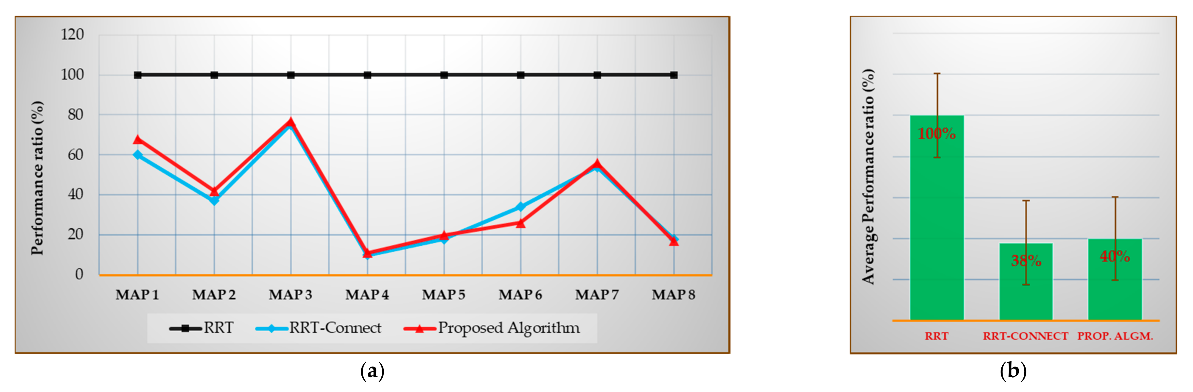
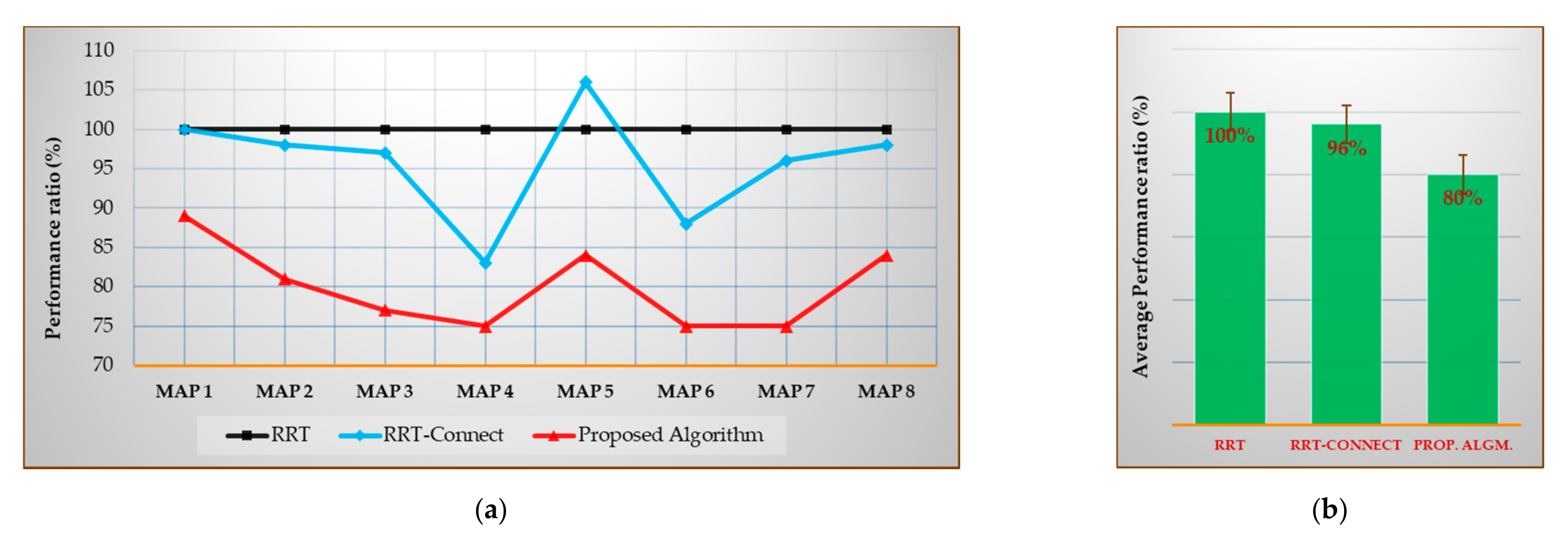
5.3. Experimental Results and Analysis in Total

This section comprehensively presents the experimental results (on average, number of samples, path length, and planning time) for each algorithm: RRT, RRT-Connect, and the proposed triangular inequality-based RRT-Connect algorithm, in the eight environmental maps (Figure 10) shown in Section 5.2.

Figures 19a–21a show the performances of the RRT-Connect algorithm and the proposed algorithm when the RRT algorithm’s performance is set to 100% for each environment map. The (b) of each figure shows the performance average of all environment maps for each algorithm. The values shown in (a) of Figures 19–21 can be expressed as in Equations (24) and (25) and the values shown in (b) can be expressed as Equation (26)

$$X_{cmp}={\displaystyle \sum }_{i=0}^{M}x{\left(i\right)}_{cmp}/M$$

(26)

Here, $X_{cmp}$ refers to the Y-axis in (b) of Figures 19–21 and M is the number of environment maps used in the experiment. The experiment in this paper includes eight maps. That is, Equation (26) shows the average value of I for all maps in Equation (25).

Figure 19 shows the average number of samples [%] compared with the RRT algorithm for Maps 1–8 (after repeating the trial 50 times) and the average number of samples [%] compared with the average result of each algorithm for each map (after repeating the trials 50 times) when the result of RRT algorithm is considered 100%.

As shown in Figure 19b, the average number of samples for all environment maps was 38% less in the RRT-Connect algorithm and 40% less in the proposed algorithm compared to the RRT algorithm. The proposed algorithm is 2% less efficient than the RRT-Connect algorithm.

Table 10. Experimental results in total for the average number of samples (for first path finding) [%].

Algorithm (cmp)	Performance Ratio Based on RRT $\left({\mathit{x}}_{\mathit{c}\mathit{m}\mathit{p}}\left(\mathit{i}\right)\right)$								Avg. $\left({\mathit{X}}_{\mathit{c}\mathit{m}\mathit{p}}\right)$
	Map 1	Map 2	Map 3	Map 4	Map 5	Map 6	Map 7	Map 8
RRT	100	100	100	100	100	100	100	100	100
RRT-Connect	60	37	75	10	18	34	54	18	38
Proposed	68	42	77	11	20	26	56	17	40

is the data table of Figure 19a. The proposed algorithm shows better performance than the RRT-Connect algorithm for Maps 6 and 8 and the RRT-Connect algorithm shows better performance than the proposed algorithm in Maps 1–5 and 7. However, the difference is not significant for most of the maps, such as showing a 2% difference from the map average. There are cases in which the proposed algorithm is 1–8% better than the RRT-Connect algorithm and there are cases in which the RRT-Connect algorithm is 1–8% better than the proposed algorithm.

Figure 20 shows the average path length [%] compared to the RRT algorithm for Maps 1–8 (after repeating the trials 50 times), and the average path length (%) compared with the average result of each algorithm for each map (again after repeating the trials 50 times) where the result of the RRT algorithm was considered as 100%.

As shown in Figure 20b, the average path length for all environment maps was 96% less in the RRT-Connect algorithm and 80% less in the proposed algorithm compared to the RRT algorithm. The proposed algorithm is 16% more efficient than the RRT-Connect algorithm.

Table 11. Experimental results in total on the average path length (%).

Algorithm (cmp)	Performance Ratio Based on RRT $\left({\mathit{x}}_{\mathit{c}\mathit{m}\mathit{p}}\left(\mathit{i}\right)\right)$								Avg. $\left({\mathit{X}}_{\mathit{c}\mathit{m}\mathit{p}}\right)$
	Map 1	Map 2	Map 3	Map 4	Map 5	Map 6	Map 7	Map 8
RRT	100	100	100	100	100	100	100	100	100
RRT-Connect	100	98	97	83	106	88	96	98	96
Proposed	89	81	77	75	84	75	75	84	80

is the data table of Figure 20a. The proposed algorithm shows better performance than the RRT-Connect algorithm for all maps. The proposed algorithm is 8–21% better than the RRT-Connect algorithm.

Figure 21 shows the average planning time [%] compared to the RRT algorithm for each map (after repeating the trials 50 times), and the average planning time (%) compared with the average result of each algorithm for each map (after repeating the trials 50 times) when the result of RRT algorithm is considered 100%.

As shown in Figure 21b, the average planning time for all environment maps was 51% less in the RRT-Connect algorithm and 53% less in the proposed algorithm compared to the RRT algorithm. The proposed algorithm was 2% less efficient than the RRT-Connect algorithm.

Table 12. Experimental results in total for the average planning time (%).

Algorithm (cmp)	Performance Ratio Based on RRT $\left({\mathit{x}}_{\mathit{c}\mathit{m}\mathit{p}}\left(\mathit{i}\right)\right)$								Avg. $\left({\mathit{X}}_{\mathit{c}\mathit{m}\mathit{p}}\right)$
	Map 1	Map 2	Map 3	Map 4	Map 5	Map 6	Map 7	Map 8
RRT	100	100	100	100	100	100	100	100	100
RRT-Connect	58	50	35	100	15	67	80	3	51
Proposed	83	50	36	133	15	44	60	3	53

is the data table of Figure 21a. The proposed algorithm shows the same or better performance for Maps 2 and 5–8 than the RRT-Connect algorithm. It shows worse performance for Maps 1, 3, and 4 than the RRT-Connect algorithm. However, most of the maps show no significant difference, such as showing a 2% difference from the map average. There are cases in which the proposed algorithm is 20–23% better than the RRT-Connect algorithm and there are cases where the RRT-Connect algorithm is 1–33% better than the proposed algorithm.

6. Conclusions

In this paper, we proposed a triangular inequality-based RRT-Connect algorithm using triangular inequality principles to overcome the limitations in the optimality of the RRT-Connect algorithm. We verified the validity of the ‘Triangular-Rewiring’ method based on the triangular inequality principle and applied it to the RRT-Connect algorithm to bring it closer to the optimum. In addition, to check performance indicators such as the number of samples for finding the first path, path length, and planning time of the proposed algorithm, we compared between the RRT and RRT-Connect algorithms across a total of eight environments through simulation. On average, the proposed algorithm showed 20% better efficiency than the RRT algorithm and 16% better efficiency than the RRT-Connect algorithm in path length and 47% better efficiency than the RRT algorithm in planning time but 2% worse efficiency than the RRT-Connect algorithm. In conclusion, the proposed algorithm showed shorter paths than the RRT-Connect algorithm with a similar number of samples and planning time.

However, one of the limitations of the proposed algorithm is the Kinodynamic planning problem [17]. When the intermediate node disappears by ‘Triangular-Rewiring’ method, a non-differentiable piecewise linear section with sharp corner may occurs, which cause a problem related with the kinematic constraint of the robot.

References

1. Schwab, K. The Fourth Industrial Revolution; Crown Business: New York, NY, USA, 2017. [Google Scholar]
2. Sariff, N.; Buniyamin, N. An overview of autonomous mobile robot path planning algorithms. In Proceedings of the IEEE 4th Student Conference on Research and Development, Selangor, Malaysia, 28–29 June 2006; pp. 183–188. [Google Scholar]
3. Roy, D. Visibility graph based spatial path planning of robots using configuration space algorithms. Int. J. Robot. Autom. 2009, 24, 1–9. [Google Scholar] [CrossRef]
4. Katevas, N.I.; Tzafestas, S.G.; Pnevmatikatos, C.G. The approximate cell decomposition with local node refinement global path planning method: Path nodes refinement and curve parametric interpolation. J. Intell. Robot. Syst. 1998, 22, 289–314. [Google Scholar] [CrossRef]
5. Warren, C.W. Global Path Planning using Artificial Potential Fields. In Proceedings of the International Conference on Robotics and Automation, Scottsdale, AZ, USA, 14–19 May 1989; Volume 1, pp. 316–321. [Google Scholar]
6. LaValle, S.M. Motion planning part II: Wild frontiers. IEEE Robot. Autom. Mag. 2011, 18, 108–118. [Google Scholar]
7. Mac, T.T.; Copot, C.; Tran, D.T.; De Keyser, R. Heuristic approaches in robot path planning: A survey. Robot. Auton. Syst. 2016, 86, 13–28. [Google Scholar] [CrossRef]
8. Paden, B.; Čáp, M.; Yong, S.Z.; Yershov, D.; Frazzoli, E. A survey of motion planning and control techniques for self-driving urban vehicles. IEEE Trans. Intell. Veh. 2016, 1, 33–55. [Google Scholar] [CrossRef] [Green Version]
9. Karaman, S.; Frazzoli, E. Incremental sampling based algorithms for optimal motion planning. arXiv 2010, arXiv:1005.0416. [Google Scholar]
10. Brunner, M.; Bruggemann, B.; Schulz, D. Hierarchical Rough Terrain Motion Planning using an Optimal Sampling based Method. In Proceedings of the IEEE International Conference on Robotics and Automation, Karlsruhe, Germany, 6–10 May 2013; pp. 5539–5544. [Google Scholar]
11. Adiyatov, O.; Varol, H.A. Rapidly-exploring Random Tree Based Memory Efficient Motion Planning. In Proceedings of the IEEE International Conference on Mechatronics and Automation, Takamatsu, Japan, 4–7 August 2013; pp. 354–359. [Google Scholar]
12. LaValle, S.M.; Kuffner, J.J., Jr. Randomized kinodynamic planning. Int. J. Robot. Res. 2001, 20, 378–400. [Google Scholar] [CrossRef]
13. LaValle, S.M. Rapidly-Exploring Random Trees: A New Tool for Path Planning; Springer: London, UK, 1998. [Google Scholar]
14. Englot, B.; Hover, F.S. Sampling based coverage path planning for inspection of complex structures. In Proceedings of the ICAPS 2012, 22nd International Conference on Automated Planning and Scheduling, Atibaia, Sao Paulo, Brazil, 25–29 June 2012. [Google Scholar]
15. Kuffner, J.J., Jr.; LaValle, S.M. RRT-connect: An Efficient Approach to Single-query Path Planning. In Proceedings of the IEEE International Conference on Robotics and Automation, San Francisco, CA, USA, 24–28 April 2000; Volume 2, pp. 995–1001. [Google Scholar]
16. Islam, F.; Nasir, J.; Malik, U.; Ayaz, Y.; Hasan, O. Rrt*-smart: Rapid Convergence Implementation of rrt* towards Optimal Solution. In Proceedings of the IEEE International Conference on Mechatronics and Automation, Chengdu, China, 5–8 August 2012; pp. 1651–1656. [Google Scholar]
17. Jeong, I.-B.; Lee, S.-J.; Kim, J.-H. Quick-RRT*: Triangular inequality based implementation of RRT* with improved initial solution and convergence rate. Expert Syst. Appl. 2019, 123, 82–90. [Google Scholar] [CrossRef]
18. Karaman, S.; Frazzoli, E. Sampling based algorithms for optimal motion planning. Int. J. Robot. Res. 2011, 30, 846–894. [Google Scholar] [CrossRef]
19. Gammell, J.D.; Srinivasa, S.S.; Barfoot, T.D. Informed RRT*: Optimal Sampling based Path Planning Focused via Direct Sampling of an Admissible Ellipsoidal Heuristic. In Proceedings of the IEEE/RSJ International Conference on Intelligent Robots and Systems, Chicago, IL, USA, 14–18 September 2014; pp. 2997–3004. [Google Scholar]
20. Klemm, S.; Oberländer, J.; Hermann, A.; Roennau, A.; Schamm, T.; Zollner, J.M.; Dillmann, R. RRT*-Connect: Faster, Asymptotically Optimal Motion Planning. In Proceedings of the IEEE International Conference on Robotics and Biomimetics, Zhuhai, China, 6–9 December 2015; pp. 1670–1677. [Google Scholar]
21. Choudhury, S.; Scherer, S.; Singh, S. RRT*-AR: Sampling based Alternate Routes Planning with Applications to Autonomous Emergency Landing of a Helicopter. In Proceedings of the IEEE International Conference on Robotics and Automation, Karlsruhe, Germany, 6–10 May 2013; pp. 3947–3952. [Google Scholar]
22. Noreen, I.; Amna, K.; Zulfiqar, H. A comparison of RRT, RRT* and RRT*-smart path planning algorithms. Int. J. Comput. Sci. Netw. Secur. 2016, 16, 20. [Google Scholar]
23. Da Silva Arantes, M.; Toledo, C.F.M.; Williams, B.C.; Ono, M. Collision-free encoding for chance-constrained nonconvex path planning. IEEE Trans. Robot. 2019, 35, 433–448. [Google Scholar] [CrossRef]
24. Nazarahari, M.; Khanmirza, E.; Doostie, S. Multi-objective multi-robot path planning in continuous environment using an enhanced genetic algorithm. Expert Syst. Appl. 2019, 115, 106–120. [Google Scholar] [CrossRef]
25. Sung, I.; Choi, B.; Nielsen, P. On the training of a neural network for online path planning with offline path planning algorithms. Int. J. Inf. Manag. 2020, 102142. [Google Scholar] [CrossRef]
26. Jeon, G.-Y.; Jung, J.-W. Water sink model for robot motion planning. Sensors 2019, 19, 1269. [Google Scholar] [CrossRef] [PubMed] [Green Version]
27. Han, J. Mobile robot path planning with surrounding point set and path improvement. Appl. Soft Comput. 2017, 57, 35–47. [Google Scholar] [CrossRef]
28. Yoon, H.U.; Lee, D.-W. Subplanner algorithm to escape from local minima for artificial potential function based robotic path planning. Int. J. Fuzzy Log. Intell. Syst. 2018, 18, 263–275. [Google Scholar] [CrossRef]
29. Jung, J.-W.; So, B.-C.; Kang, J.-G.; Lim, D.-W.; Son, Y. Expanded Douglas–Peucker polygonal approximation and opposite angle based exact cell decomposition for path planning with curvilinear obstacles. Appl. Sci. 2019, 9, 638. [Google Scholar] [CrossRef] [Green Version]
Figure 1. Overview of the algorithms in this paper: (a) RRT; (b) RRT-Connect; (c) the proposed algorithm.
Sensors 21 00333 g001
Figure 2. RRT algorithm: (a) Process when qnew is created; (b) After the random sampling has ended.
Sensors 21 00333 g002
Figure 3. The ‘Extend’ method from RRT-Connect algorithm.
Sensors 21 00333 g003
Figure 4. The ‘Connect’ method from the RRT-Connect algorithm.
Sensors 21 00333 g004
Figure 5. Abstract process of the ‘Triangular-Rewiring’ method: (a) Example tree; (b) After rewiring between qchild and qancestor; (c) At this time, α is the distance between qchild and qparent, β is the distance between qparent and qancestor, and γ is the distance between qchild and qancestor.
Sensors 21 00333 g005
Figure 6. Detailed process of the ‘Triangular-Rewiring’ method: (a) Each node q for index i (at this time, qstart is same as q7 and qgoal is same as q0); (b) Represent each node using the n-th ancestor ξ n of q0; (c) Each distance 𝕕 n between the n-th and (n + 1)-th ancestor nodes of q0; (d) When the ‘Triangular-Rewiring’ method is applied and rewired by distance 𝕦 k j ; (e) Represent as the value of kj; (f) Represent each node by the n-th ancestor ξ n of q0 after method is applied.
Sensors 21 00333 g006
Figure 7. Proposed ‘Extend’ method for the RRT-Connect algorithm.
Sensors 21 00333 g007
Figure 8. Proposed ‘Connect’ method for the RRT-Connect algorithm.
Sensors 21 00333 g008
Figure 9. Detailed process of the proposed algorithm: (a) Start position qstart from tree Ta and goal position qgoal from tree Tb; (b) Create qnewA nearest to Ta from 1st random sampling position qrand and create qnewB from qgoal nearest to Tb; (c) Create new qnewA from qnear nearest to Tb from the second random sampling position qrand and rewire between qnewA and qgoal the ancestor of the qnewA; (d) Create a new qnewA from qnear nearest to Ta from the third random sampling position qrand and rewire between qnewA and qstart with the ancestor of qnewA; (e) Create new qnewA from qnear nearest to Ta from the fifth random sampling position qrand and connect between qnewA and qnewB nearest to Tb from qnewA; (f) Result of Path R from qstart to qgoal.
Sensors 21 00333 g009
Figure 10. Maps for the experiment: (a) Map 1; (b) Map 2; (c) Map 3; (d) Map 4; (e) Map 5; (f) Map 6; (g) Map 7; (h) Map 8.
Sensors 21 00333 g010
Figure 11. Experimental result of Map 1: (a) RRT; (b) RRT-Connect; (c) the proposed algorithm.
Sensors 21 00333 g011
Figure 12. Experimental results of Map 2: (a) RRT; (b) RRT-Connect; (c) the proposed algorithm.
Sensors 21 00333 g012
Figure 13. Experimental result of Map 3: (a) RRT; (b) RRT-Connect; (c) the proposed algorithm.
Sensors 21 00333 g013
Figure 14. Experimental result of Map 4: (a) RRT; (b) RRT-Connect; (c) the proposed algorithm.
Sensors 21 00333 g014
Figure 15. Experimental result of Map 5: (a) RRT; (b) RRT-Connect; (c) the proposed algorithm.
Sensors 21 00333 g015
Figure 16. Experimental result of Map 6: (a) RRT; (b) RRT-Connect; (c) the proposed algorithm.
Sensors 21 00333 g016
Figure 17. Experimental result of Map 7: (a) RRT; (b) RRT-Connect; (c) the proposed algorithm.
Sensors 21 00333 g017
Figure 18. Experimental result of Map 8: (a) RRT; (b) RRT-Connect; (c) the proposed algorithm.
Sensors 21 00333 g018
Figure 19. Experimental results in total for the average number of samples (for first path finding): (a) result of each map compared with the RRT algorithm ( x c m p i ); (b) average result compared with the RRT algorithm ( X c m p ).
Sensors 21 00333 g019
Figure 20. Experimental results in total for the average path length: (a) result of each map compared with the RRT algorithm ( x c m p i ); (b) average result compared with the RRT algorithm ( X c m p ).
Sensors 21 00333 g020
Figure 21. Experimental results in total on the average planning time: (a) result of each map compared with the RRT algorithm ( x c m p i ); (b) average result compared to the RRT algorithm ( X c m p ).
Sensors 21 00333 g021