We simulated many conditions to validate the accuracy of our method. Firstly, the variation of the intersection angle of the two cameras and the 3D line’s attitude variation were simulated to verify the accuracy and robustness of the proposed algorithm. Secondly, the various error conditions for the stereo vision were simulated, including the 2D line extraction error, the external camera parameter error, and both the above errors. Thirdly, we verified the accuracy while in a multiple camera system. Finally, we assessed the time performance of our method in a multiple camera system.
4.1.3. Simulation Results
The simulation details and results are given, respectively.
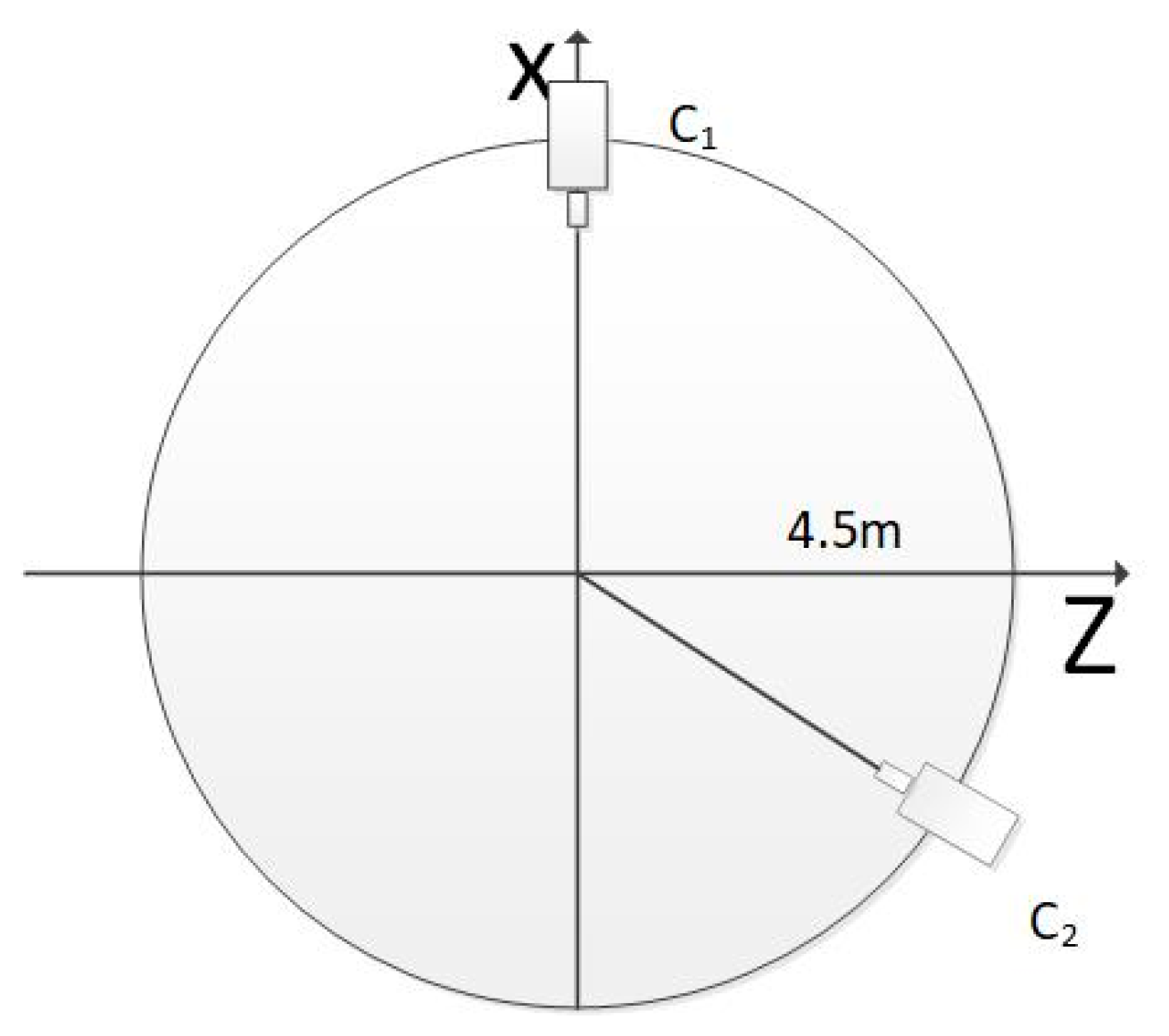
Firstly, we simulated the intersection angles of two cameras, which varied to verify the accuracy of the three methods. As shown in
Figure 3, C
1 was placed in the fixed point (4.5,0,0), and C
2 was moved on the circle with a radius of 4.5 m. The angle between the optical axes of C
1 and C
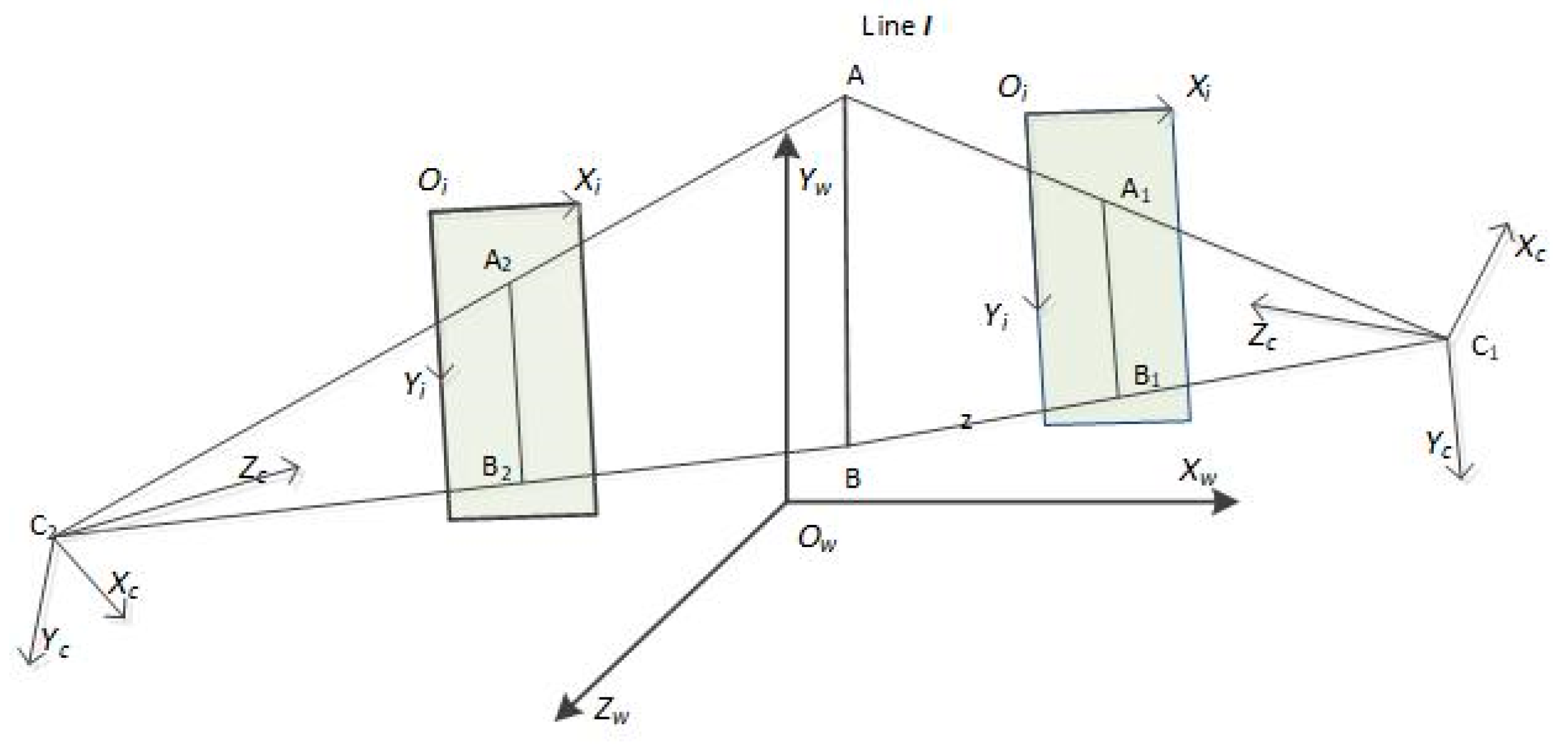
2 varied from 30° to 150°. We simulated two conditions of the 3D line, one of which was the 3D line perpendicular to the baseline of C
1 and C
2. When the 3D line was perpendicular to the baseline, the endpoints of the 3D line segment were
and
. From the definition of the simulation scenario, we knew that, as the intersection angle changed from 30° to 150°, the line segment AB was always perpendicular to the baseline, and the distance between AB and the baseline became smaller and smaller. When the 3D line is not perpendicular to the baseline, the endpoints of the 3D line segment were
,
. A Gaussian error with a mean of 0 was added to the optical center of the camera, with a 5 cm RMS value. A Gaussian error with a mean of 0 was added to the camera angle, with a 1° RMS value. A Gaussian error with a mean of 0 was added to the
x- and
y-directions of the two endpoints of the 2D line segments, with a 2-pixel RMS value. The results are shown in
Figure 4.
When the 3D line remained unchanged, the error was relevant to the intersection angle. In the beginning, the three methods achieved the same accuracy. As the intersection angle varied from 30° to 150°, the distance between the baseline and AB grew smaller and smaller. In other words, they were becoming closer and closer to each other, which meant the intersection condition was getting worse; the PtD method had the same accuracy as the DtP method. TPS had the best positional accuracy but the worst angular accuracy. In the condition where the 3D line was not parallel to the imaging plane and was not perpendicular to the baseline, PtD had higher accuracy both on the position and angle than DtP; TPS achieved the worst angular accuracy, and DtP achieved the worst positional accuracy.
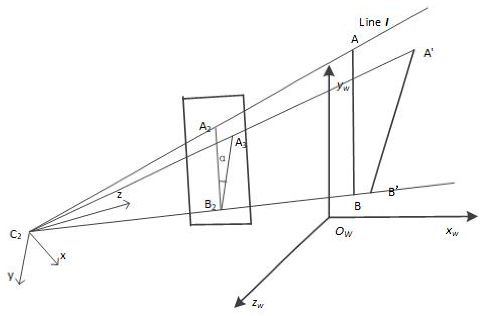
Secondly, we simulated the condition where the 3D line moved while the intersection angle remained unchanged; the C
1 and C
2 places were fixed. Endpoint A was (−0.5,−0.5,−0.5), The initial position of endpoint B was (−0.5,1.5,−0.5), and the
th position was
;
was the offset time. The end position of point B was (−5.5,1.5,−5.5). A Gaussian error with a mean of 0 was added to the optical center of the camera, with a 5 cm RMS value. A Gaussian error with a mean of 0 was added to the camera angle, with a 1° RMS value. A Gaussian error with a mean of 0 was added to the
x- and
y-directions of the two endpoints of the 2D line, with a 2-pixel RMS value. The results of the simulation while the intersection angles are 90° and 120°, and shown in
Figure 5a,b respectively.
As shown in
Figure 5, at the start, the TPS method had the best positioning accuracy and the worst angular accuracy. However, as the intersection condition became, the TPS had the best accuracy both in direction and position. The reasons are as follows.
Firstly, the 3D line became longer, and the final length was 3.68-times greater than that of the initial length. Therefore, theoretically, if only the influence of the line length was considered, the direction error of TPS would be the 1/3.68 of the original value. However, the error of the 3D point B increased because the intersection angle of 3D point B became smaller. Therefore, the error reduction was not proportional.
Secondly, the angle between the 3D line and the baseline remained unchanged—it was always 90°. However, the angle between the 3D line and the imaging plane varied from 0 to 45° and the distance between the 3D line and the baseline became smaller. At the start, when the intersection angle was 90°, the distance between the 3D line and the baseline was 3.89 m; when the intersection angle was 120°, the distance between the 3D line and the baseline was 2.94 m. At the end, however, the distances were 2.50 m and 2.30 m, respectively. The lengths of the baseline were 6.36 m and 7.79 m, respectively. From the above analysis, we can determine that the smaller distance aggravated the degeneracy of the lines’ reconstruction.
Thirdly, we simulated the condition where the cameras and the 3D line remained unchanged, but the errors of the camera’s external parameters and 2D line were different. The intersection angle was 120°. The endpoints of the 3D line were and . We simulated for 2D line error, the error of the camera external parameters, and all above errors. The error details were as below:
Case 1: A Gaussian error with a mean of 0 was added to the
x- and
y-directions at the head and the tail of the line segment, with 0–4 pixels of RMS. The results are shown in
Figure 6.
From
Figure 6, we can see that if only the same 2D line error existed, the 3D line’s accuracy of the three methods, from most to least accurate, was TPS, PtD, then DtP.
Case 2: A Gaussian error with a mean of 0 was added to the optical center of the camera, with 1 mm to 50 mm of RMS, and the step size was 1 mm. A Gaussian error with a mean of 0 was added to the camera angle, with 0.05–2.5° of RMS. The simulation results are shown in
Figure 7.
From
Figure 7, we can see that under the same error of the camera’s external parameters, the directional accuracy of the 3D line of the three methods, from most to least accurate, was PtD, DtP, then TPS, and the positional accuracy of the 3D line of the three methods from most to least accurate, was TPS, PtD, then DtP.
Case 3: A Gaussian error with a mean of 0 was added to the optical center of the camera, with 1 mm to 50 mm of RMS, and the step size was 1 mm. A Gaussian error with a mean of 0 was added to the camera angle, with 0.05–2.5° of RMS. A Gaussian error with a mean of 0 was added to the
x-and
y-directions of the two endpoints of the 3D line, with 0.1–5 pixels of RMS. The simulation results are shown in
Figure 8.
From
Figure 8, we can see that under same error of external camera’s parameters and the 2D lines, the 3D line’s direction accuracy of the three methods, from most to least accurate, was PtD, DtP, then TPS, and the 3D line’s position accuracy of the three methods, from most to least accurate, was TPS, PtD, then DtP. The position accuracies of TPS and PtD are close, and the directional accuracy of PtD was far better than TPS.
Additionally, we simulated the condition where the camera number varied from 2 to 20; the cameras were evenly distributed on the circle as shown in
Figure 3. The DtP method used the LS [
26] directly solve this scenario. A Gaussian error with a mean of 0 was added to the optical center of the camera, with a 10 mm root mean square (RMS) value. A Gaussian error with a mean of 0 was added to the camera angle, with a 0.5° RMS value. A Gaussian error with a mean of 0 was added to the
x-
y-directions of the two endpoints of the 3D line, with a 1-pixel RMS value. The endpoints of the 3D line were
. The results are shown in
Figure 9.
From
Figure 9, we can see that as the number of cameras increased, the accuracy of the three methods increased gradually, indicating that these methods utilized the constraints of the multi-camera. Similar to the result in
Figure 8, with the increase in the number of cameras, under the same error of the external camera’s parameters and the 2D lines, the 3D line’s direction accuracy of the three methods, from most to least accurate, was PtD, DtP, then TPS, and the 3D line’s positional accuracy of the three methods, from most to least accurate, was TPS, PtD, then DtP. The positional accuracies of TPS and PtD were close, and the directional accuracy of the PtD method was far better than the TPS method.
Finally, we simulated the condition where the camera number increased from 2 to 20 to verify the time performance of our method. The linear algorithm took a small amount of time; therefore, for the convenience of comparison, we counted the time it took to run 10,000 times. A Gaussian error with a mean of 0 was added to the optical center of the camera, with a 5 cm RMS value. A Gaussian error with a mean of 0 was added to the camera angle, with a 1° RMS value. A Gaussian error with a mean of 0 was added to the
x-
y-directions of the two endpoints of the 2D line segments, with a 2-pixel RMS value. The simulation results are shown in
Figure 10.
Figure 10 confirms that all three methods are linear methods; TPS took the longest, then PtD, and the fastest was DtP. DtP only needs to solve each plane equation and then solve the least-squares method; PtD needs to solve the 3D point coordinate and the line parameters in two steps; TPS needs to solve the 3D point coordinate two times, which explains the variances in running time between the methods.


