Author Contributions
Conceptualization, T.L.d.V.L., A.C.L.F. and F.A.B.; methodology, T.L.d.V.L. and A.C.L.F.; software, T.L.d.V.L., F.V.S. and T.C.B.S.; validation, T.L.d.V.L., A.C.L.F., F.A.B., K.V.M. and M.C.R.; formal analysis, T.L.d.V.L., A.C.L.F., F.A.B., K.V.M. and M.C.R.; investigation, T.L.d.V.L., F.A.B., F.V.S. and T.C.B.S.; resources, T.L.d.V.L. and A.C.L.F.; data curation, T.L.d.V.L., F.A.B., F.V.S. and T.C.B.S.; writing—original draft preparation, T.L.d.V.L. and A.C.L.F.; supervision, A.C.L.F., K.V.M. and M.C.R.; project administration, A.C.L.F. and T.L.d.V.L.; funding acquisition, A.C.L.F. All authors have read and agreed to the published version of the manuscript.
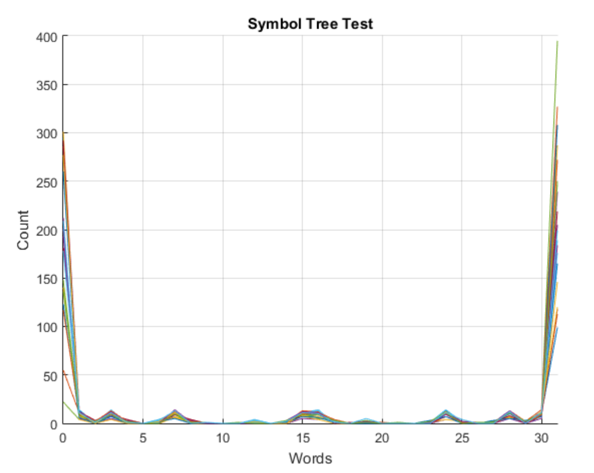
Figure 1.
Result of the symbol tree test for the sound signal under study.
Figure 1.
Result of the symbol tree test for the sound signal under study.
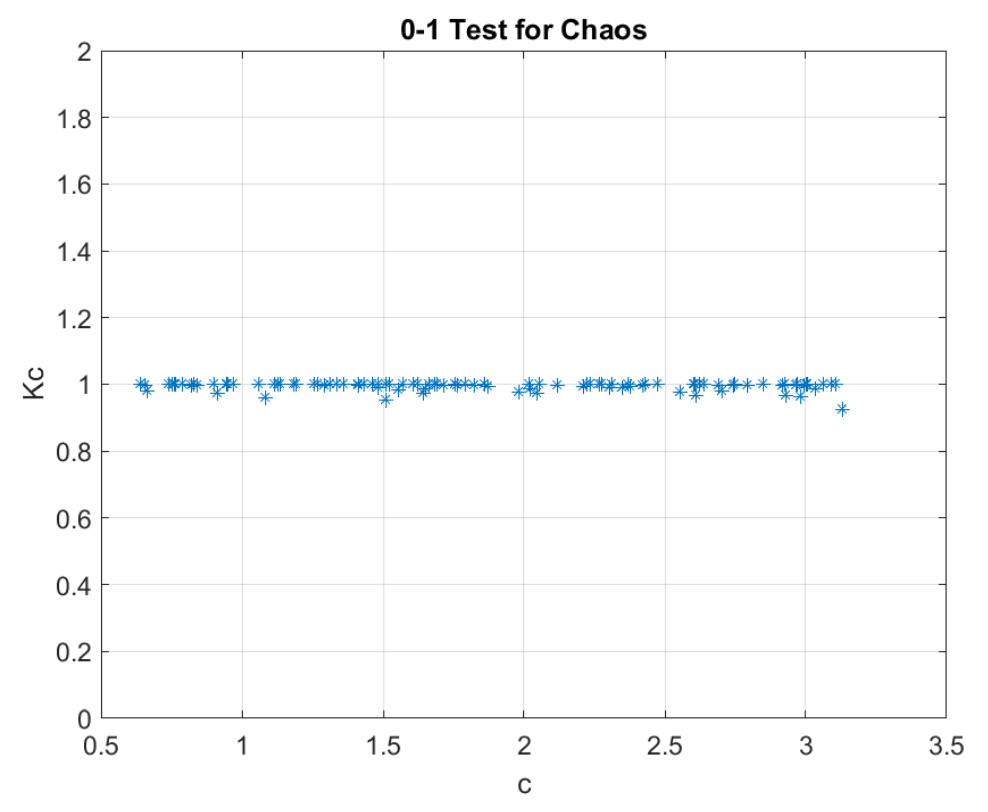
Figure 2.
Result of the 0–1 test for chaos of the sound signal under study.
Figure 2.
Result of the 0–1 test for chaos of the sound signal under study.
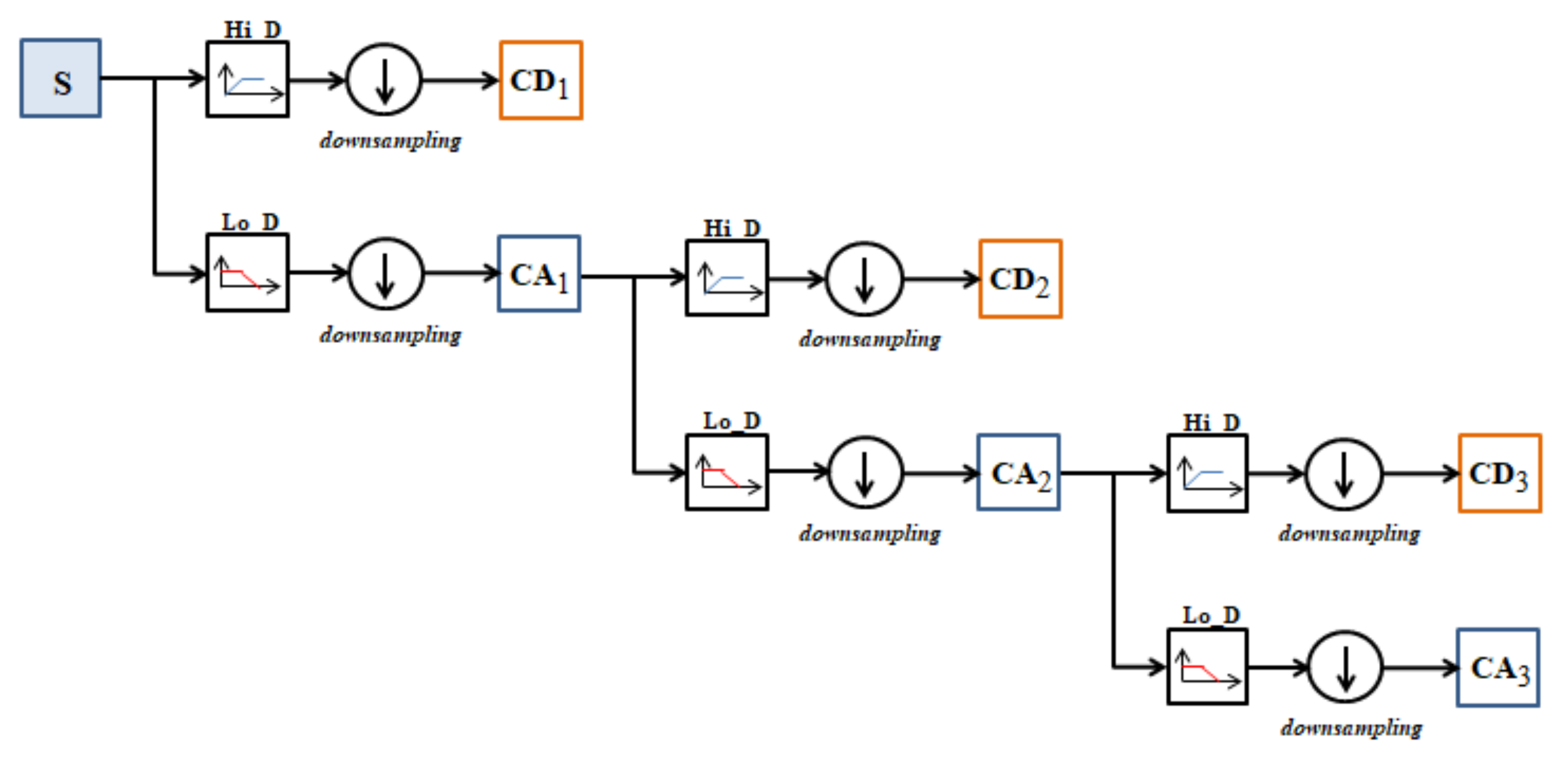
Figure 3.
Illustration of a three-level decomposition of a signal.
Figure 3.
Illustration of a three-level decomposition of a signal.
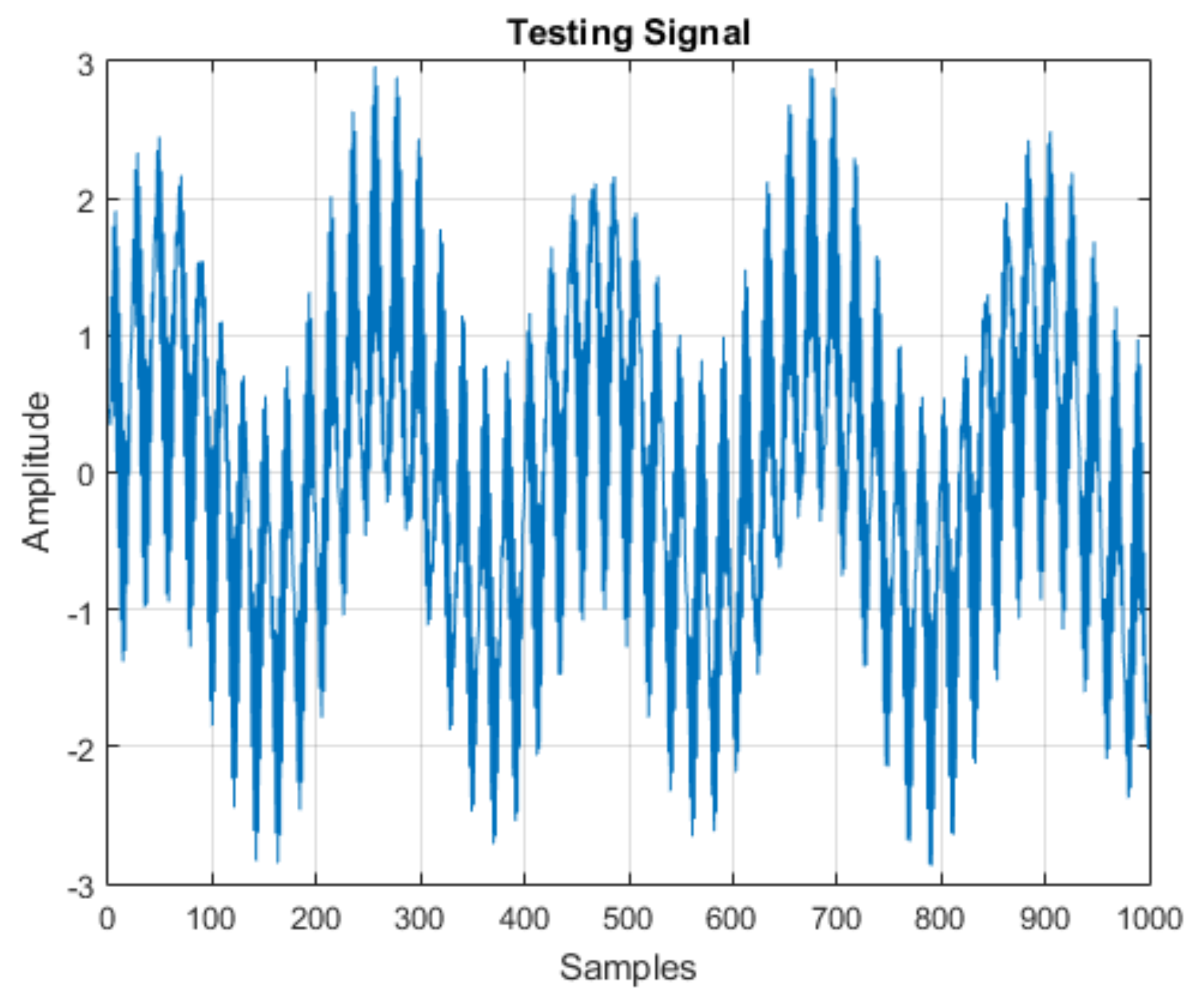
Figure 4.
Test signal for MRA.
Figure 4.
Test signal for MRA.
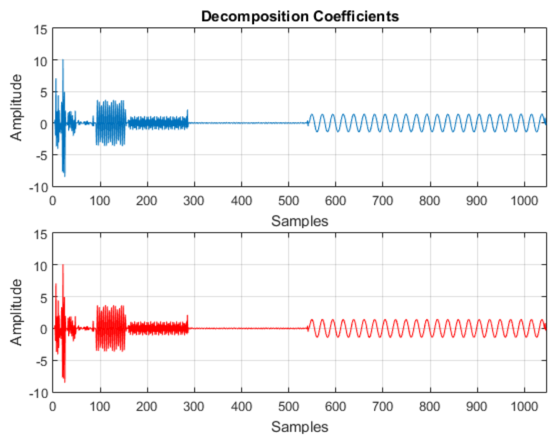
Figure 5.
Wavelet decomposition coefficients—numerical calculation software (blue) and application (red).
Figure 5.
Wavelet decomposition coefficients—numerical calculation software (blue) and application (red).
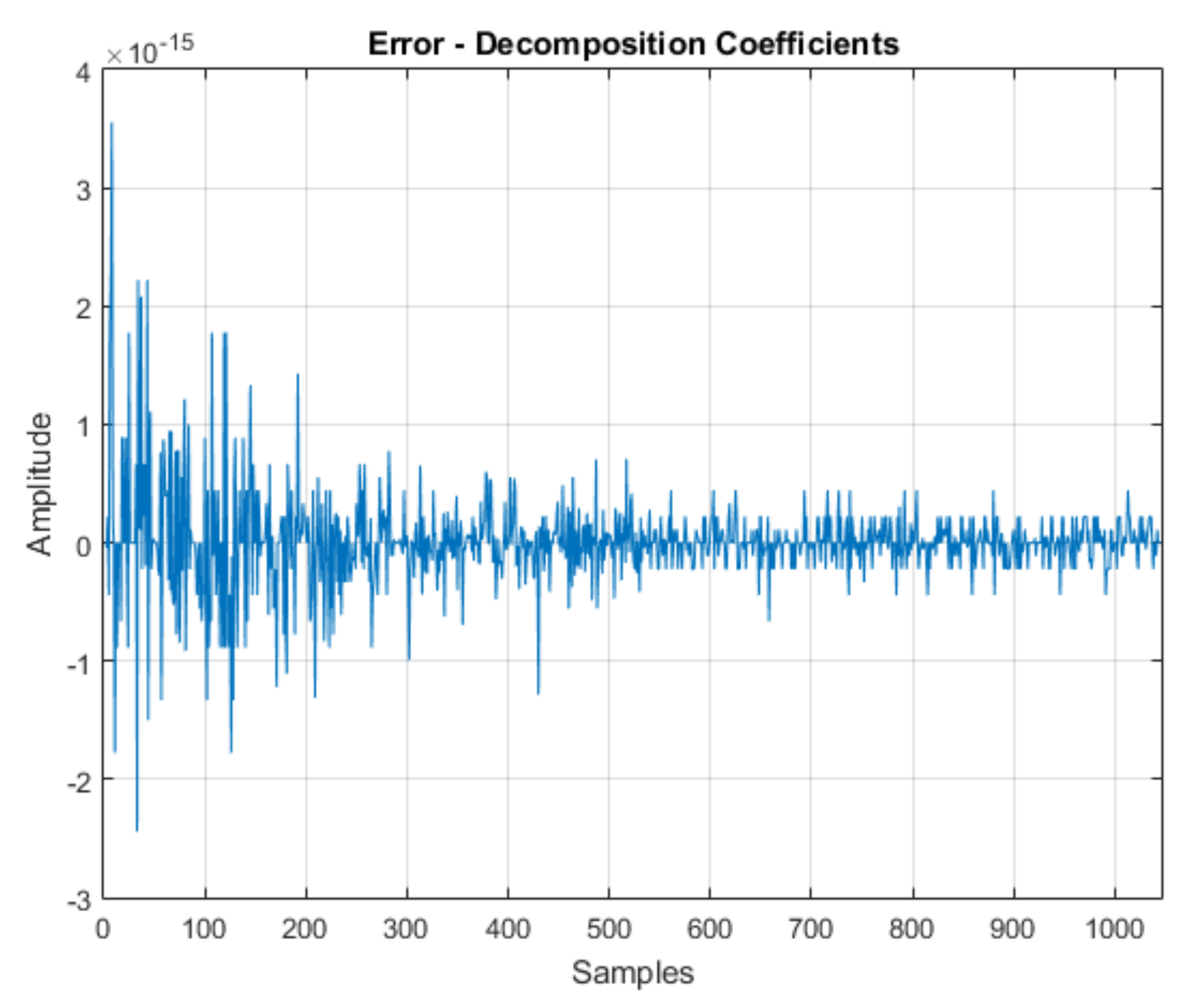
Figure 6.
Error between the numerical calculation software and application results—wavelet decomposition.
Figure 6.
Error between the numerical calculation software and application results—wavelet decomposition.
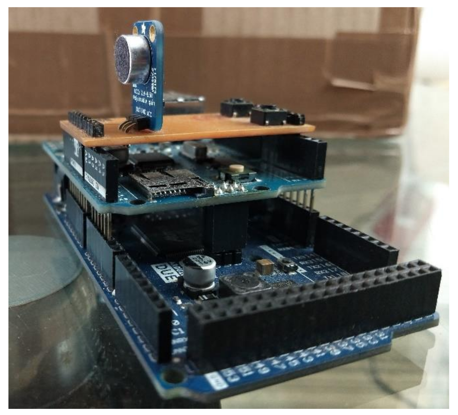
Figure 7.
Sound acquisition system.
Figure 7.
Sound acquisition system.
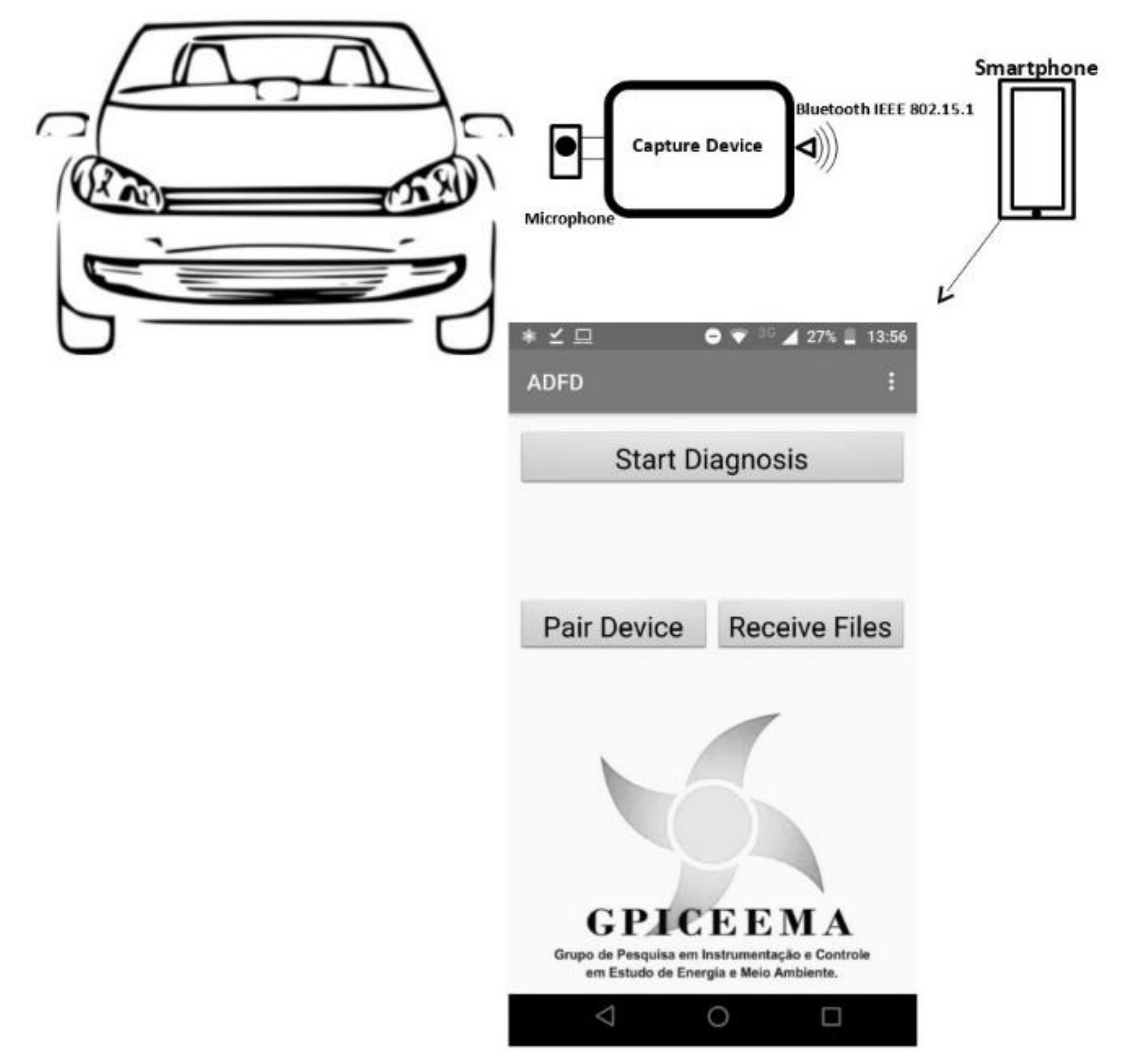
Figure 8.
Illustration of the developed system’s application.
Figure 8.
Illustration of the developed system’s application.
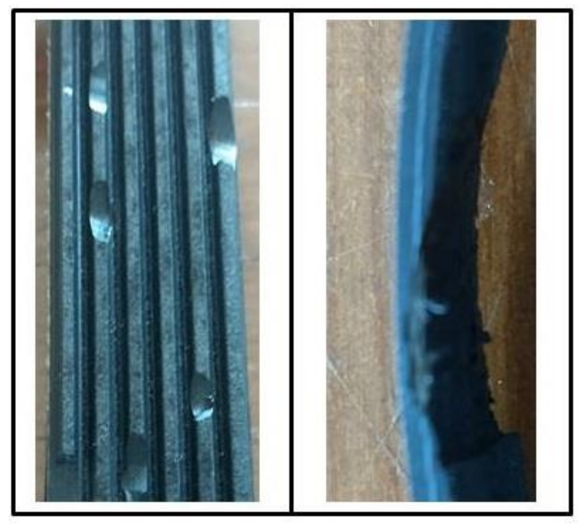
Figure 9.
BPD fault (left) and BCL fault (right).
Figure 9.
BPD fault (left) and BCL fault (right).
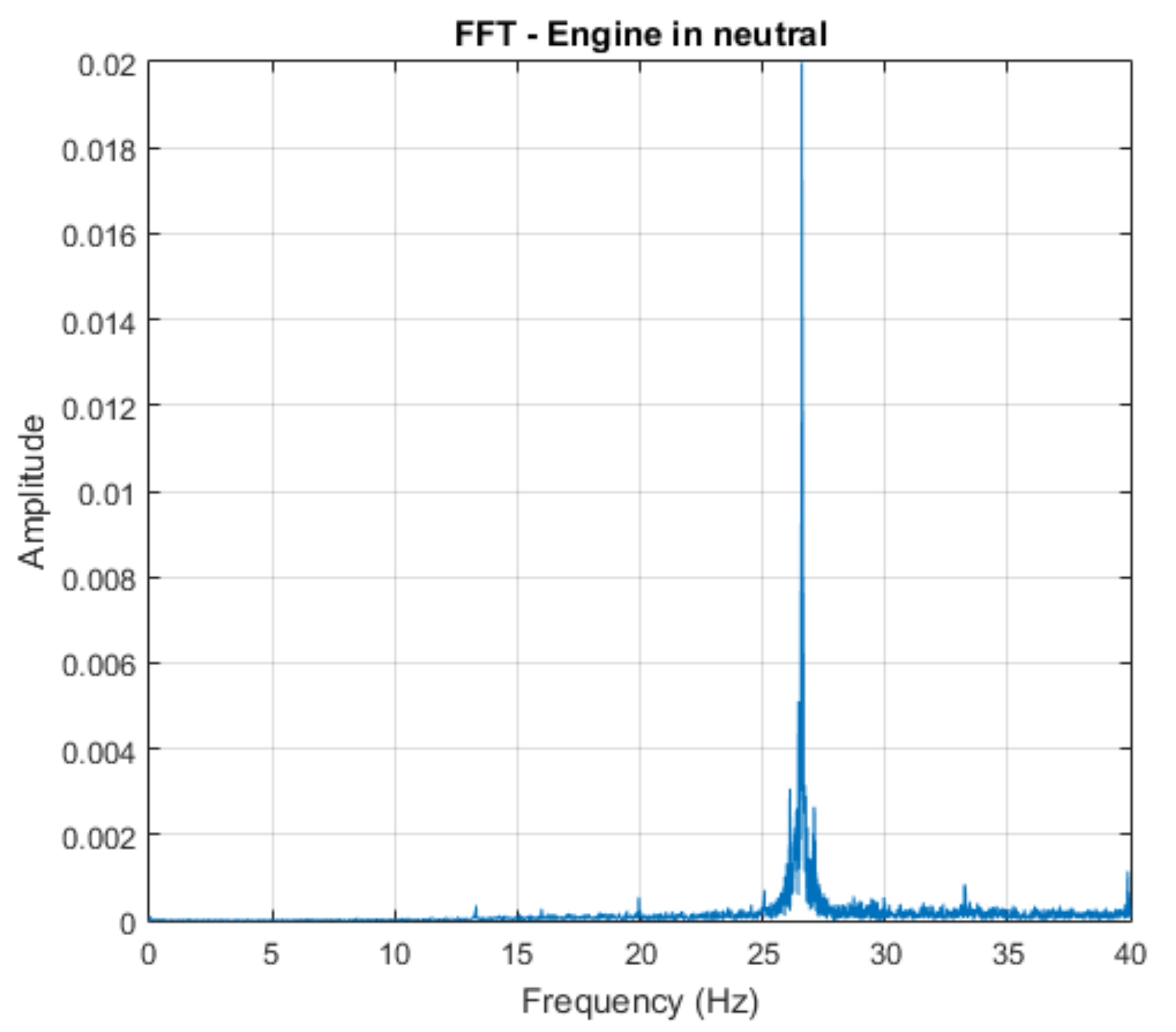
Figure 10.
FFT of the engine in neutral and in normal conditions.
Figure 10.
FFT of the engine in neutral and in normal conditions.
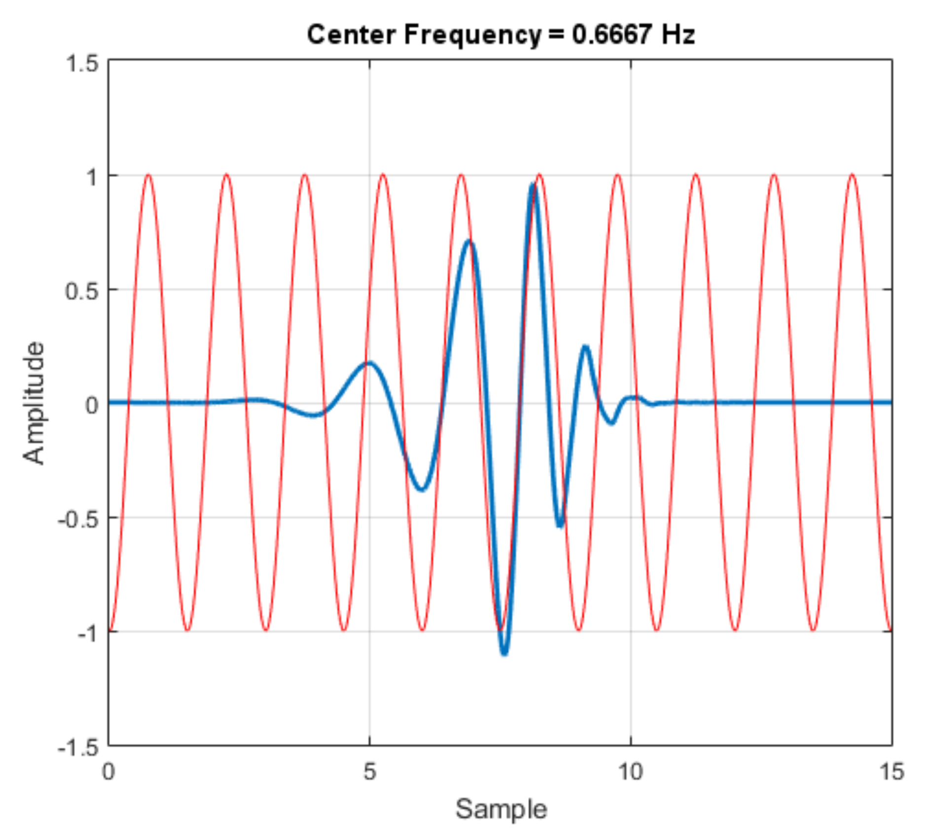
Figure 11.
Wavelet (blue) and center frequency-based approximation.
Figure 11.
Wavelet (blue) and center frequency-based approximation.
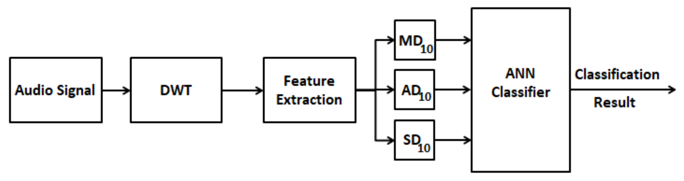
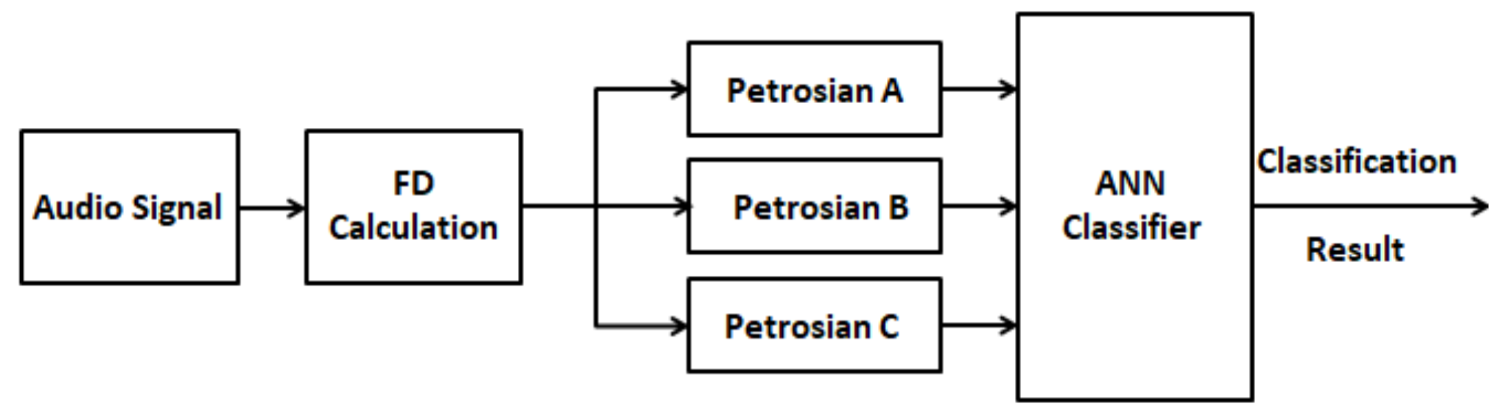
Figure 12.
Schematic of the wavelet-based method for fault detection and isolation.
Figure 12.
Schematic of the wavelet-based method for fault detection and isolation.
Figure 13.
Schematic of the wavelet-based method for fault detection and isolation.
Figure 13.
Schematic of the wavelet-based method for fault detection and isolation.
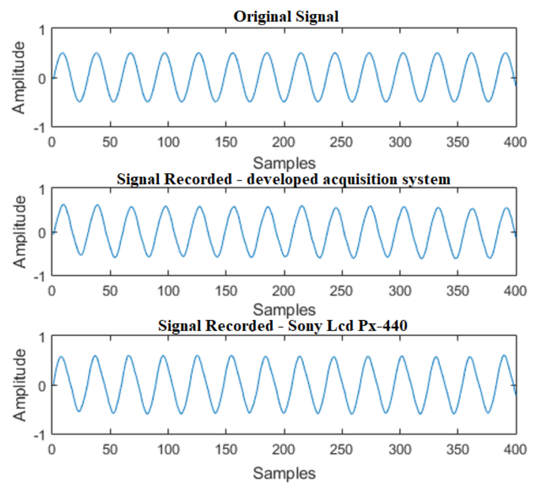
Figure 14.
Acquisition of a single tone signal—1500 Hz sine wave.
Figure 14.
Acquisition of a single tone signal—1500 Hz sine wave.
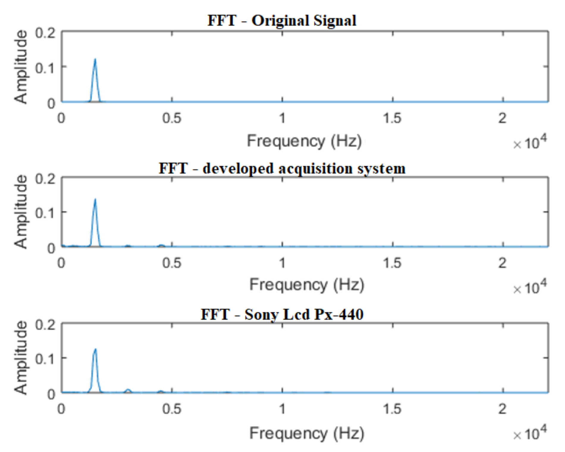
Figure 15.
FFT of a single tone signal—1500 Hz sine wave.
Figure 15.
FFT of a single tone signal—1500 Hz sine wave.
Figure 16.
Acquisition of a two-tone signal: F1 = 600 Hz/F2 = 1000 Hz.
Figure 16.
Acquisition of a two-tone signal: F1 = 600 Hz/F2 = 1000 Hz.
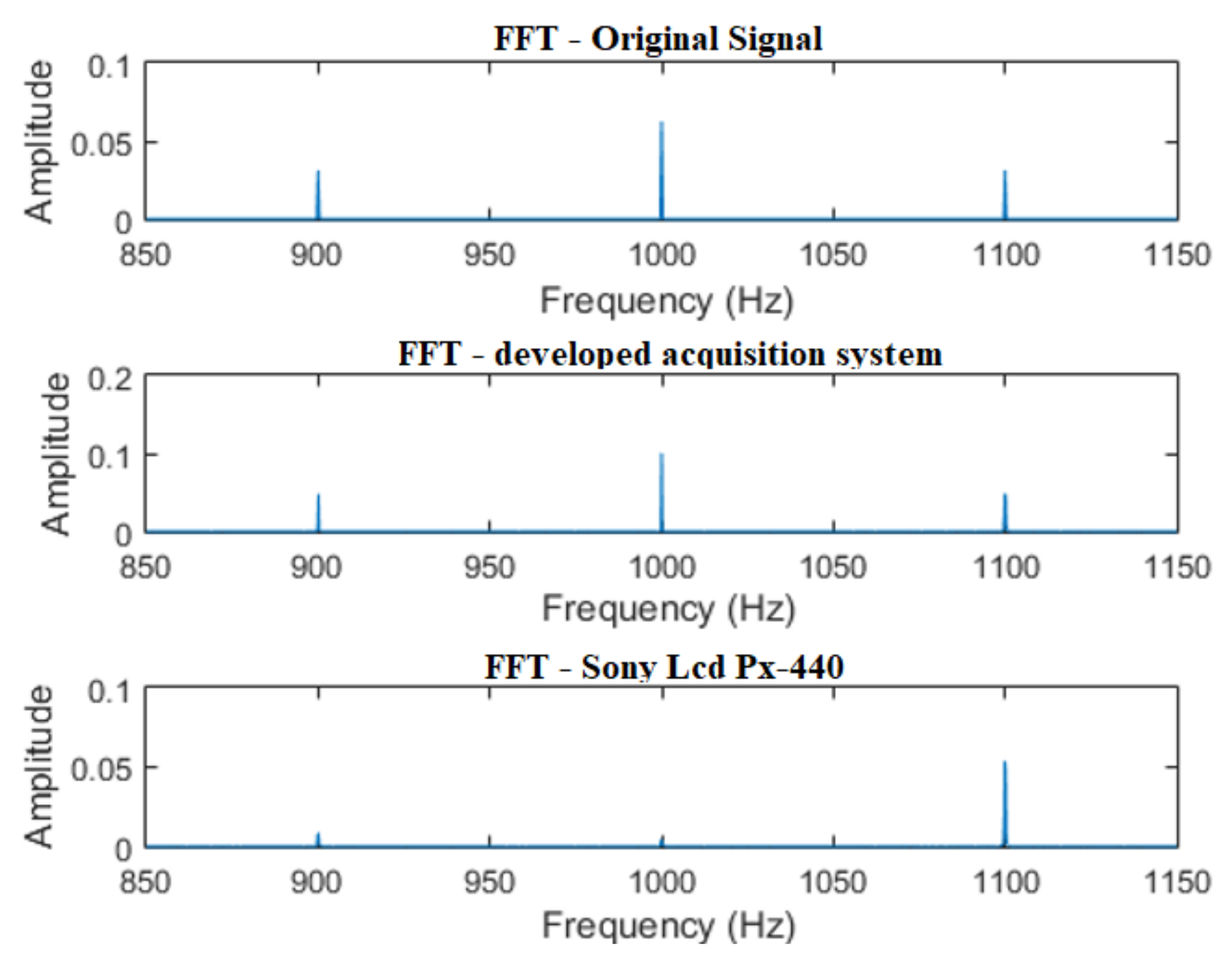
Figure 17.
FFT of a two-tone signal: F1 = 600 Hz/F2 = 1000 Hz.
Figure 17.
FFT of a two-tone signal: F1 = 600 Hz/F2 = 1000 Hz.
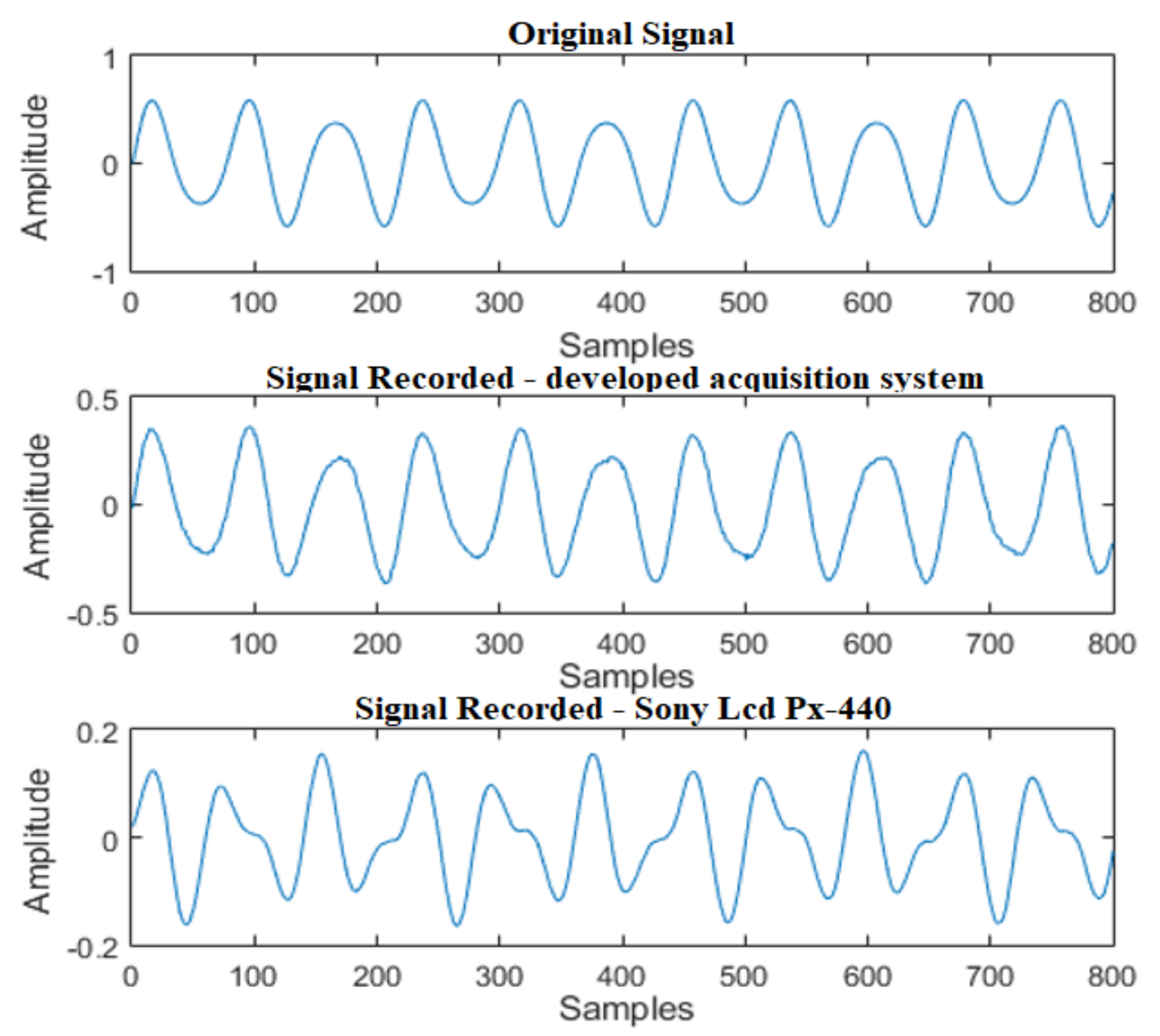
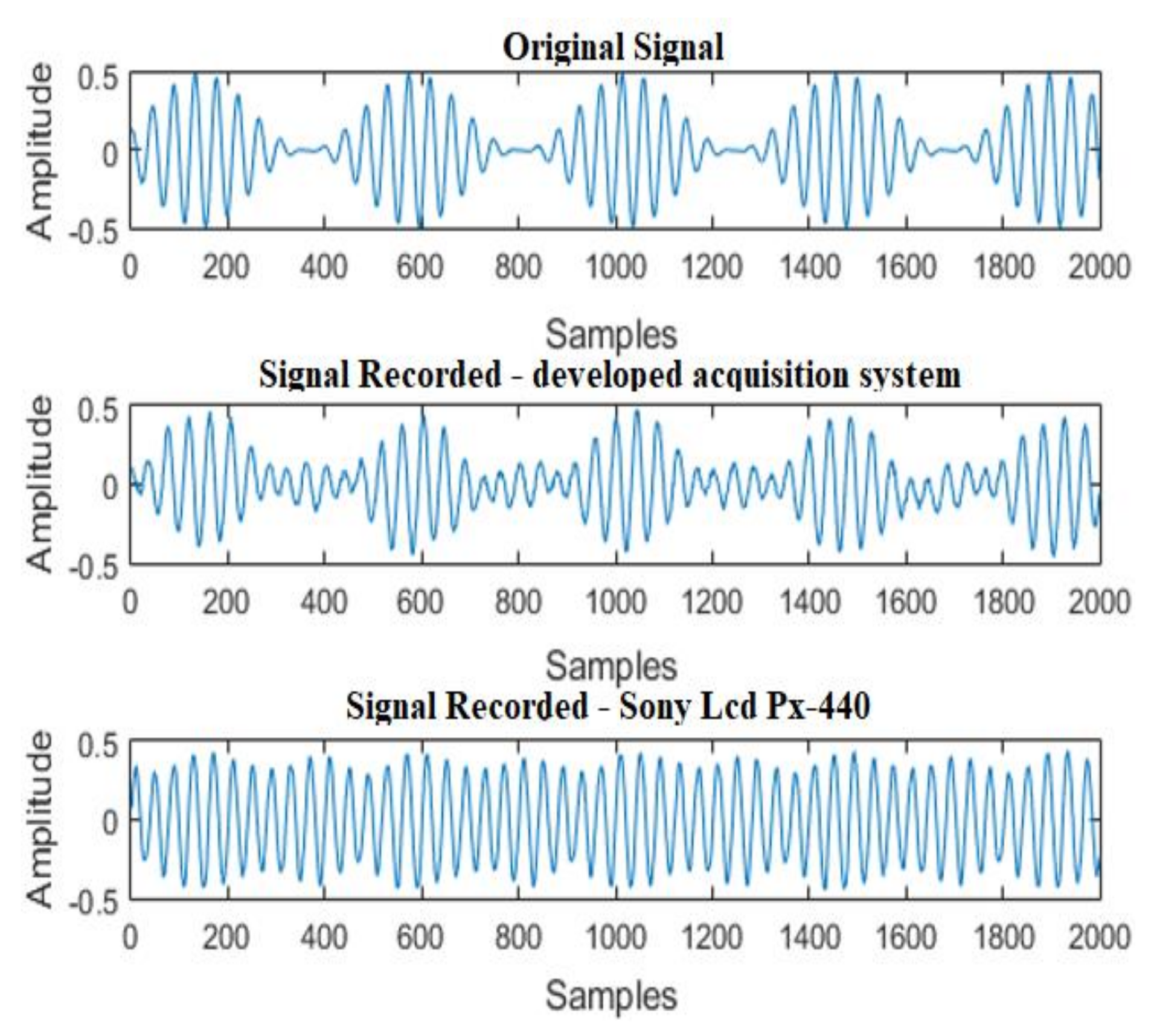
Figure 18.
Acquisition of an AM signal—carrier: 1 kHz/modulator: 100 Hz.
Figure 18.
Acquisition of an AM signal—carrier: 1 kHz/modulator: 100 Hz.
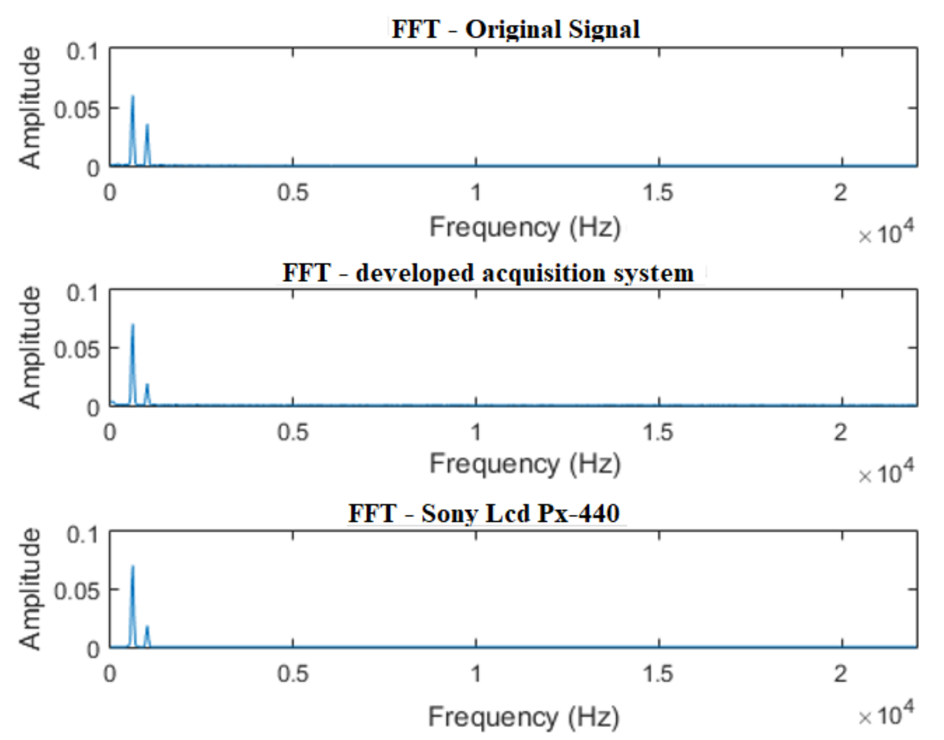
Figure 19.
FFT of an AM signal—carrier: 1 kHz/modulator: 100 Hz.
Figure 19.
FFT of an AM signal—carrier: 1 kHz/modulator: 100 Hz.
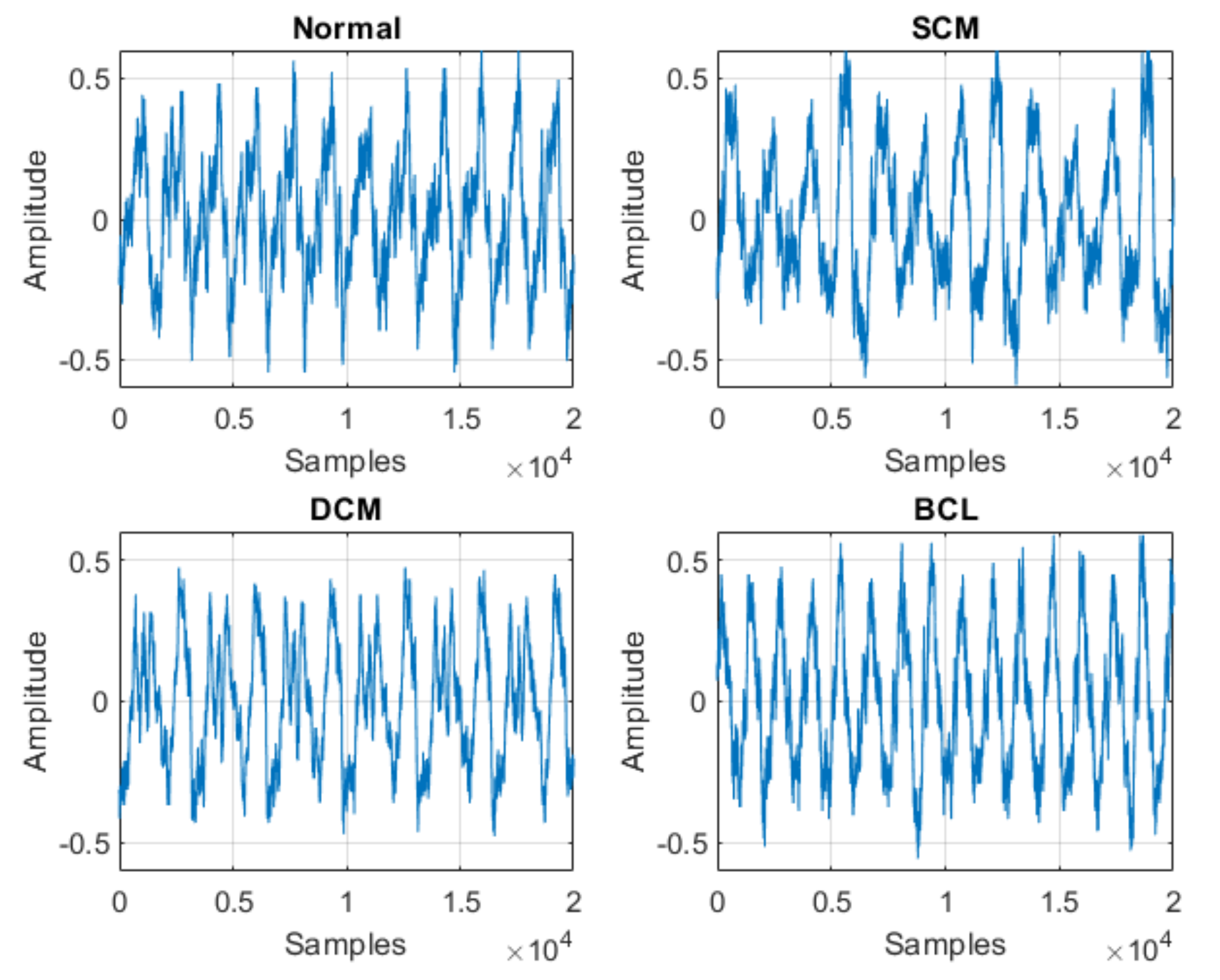
Figure 20.
Samples of the studied signals—Normal, SCM, DCM and BCL.
Figure 20.
Samples of the studied signals—Normal, SCM, DCM and BCL.
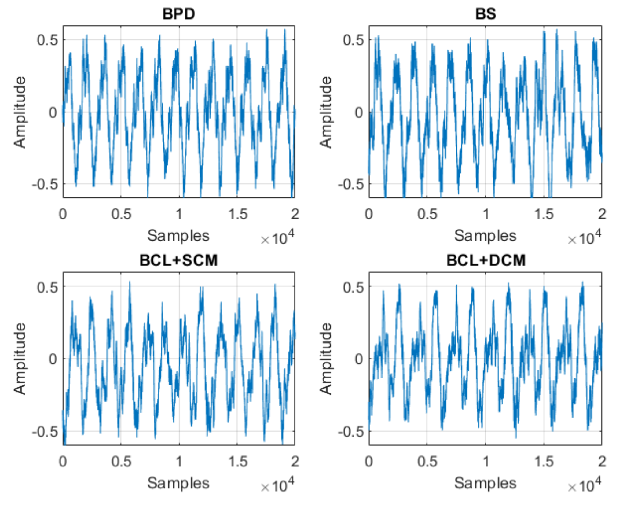
Figure 21.
Samples of the studied signals—BPD, BS, BCL + SCM and BCL + DCM.
Figure 21.
Samples of the studied signals—BPD, BS, BCL + SCM and BCL + DCM.
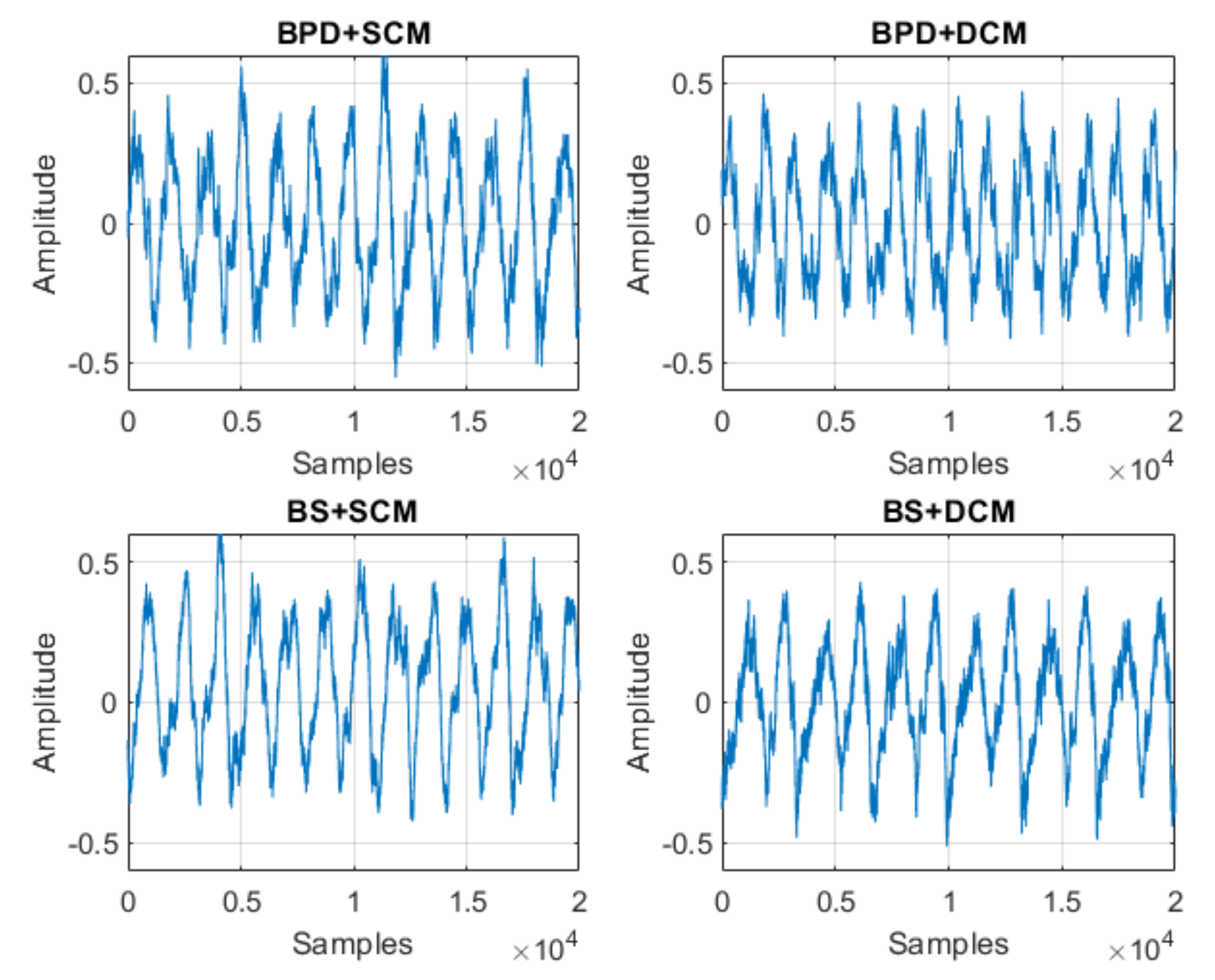
Figure 22.
Samples of the studied signals—BPD + SCM, BPD + DCM, BS + SCM and BS + DCM.
Figure 22.
Samples of the studied signals—BPD + SCM, BPD + DCM, BS + SCM and BS + DCM.
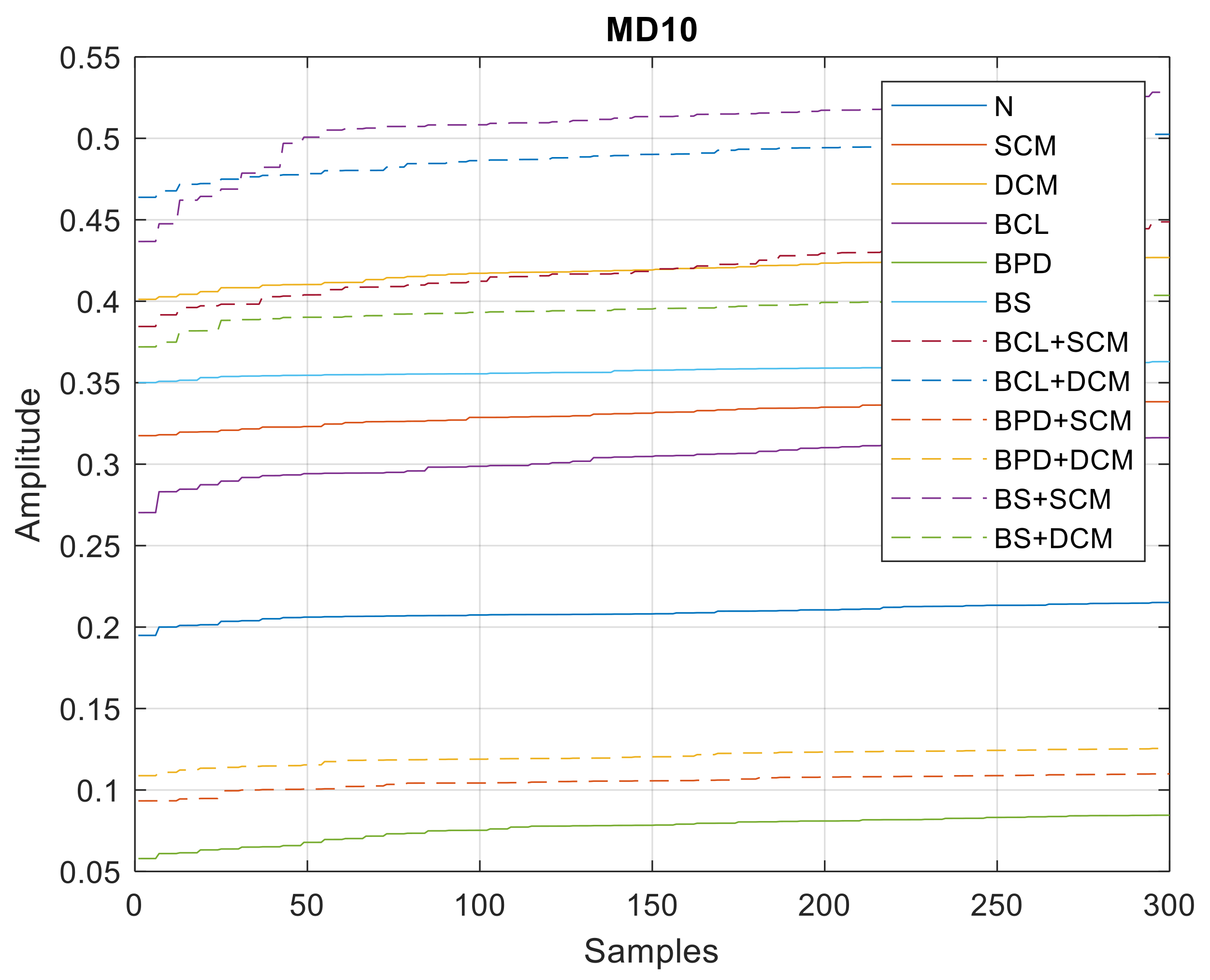
Figure 23.
MD10 values—single and double/simultaneous faults.
Figure 23.
MD10 values—single and double/simultaneous faults.
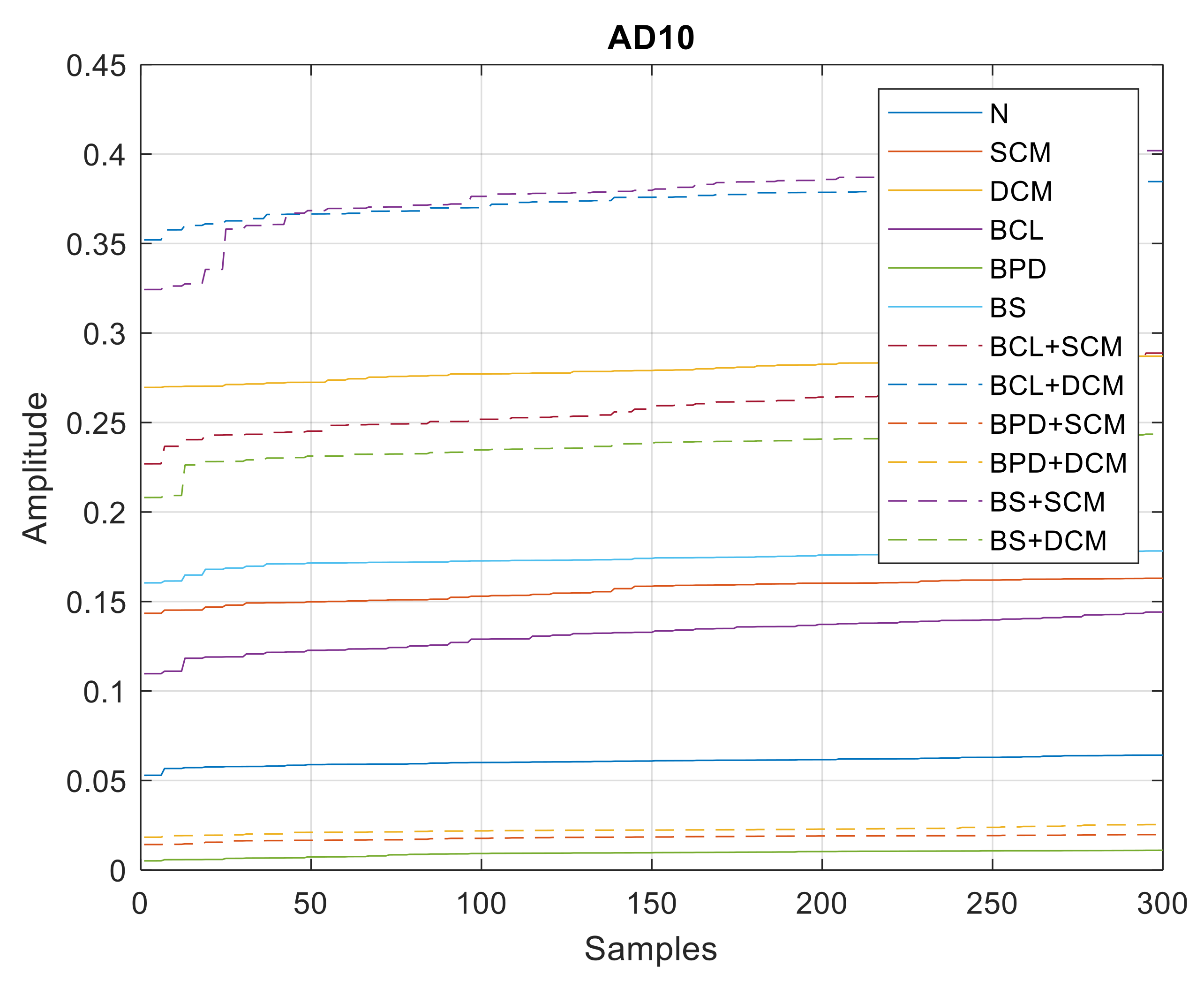
Figure 24.
AD10 values—single and double/simultaneous faults.
Figure 24.
AD10 values—single and double/simultaneous faults.
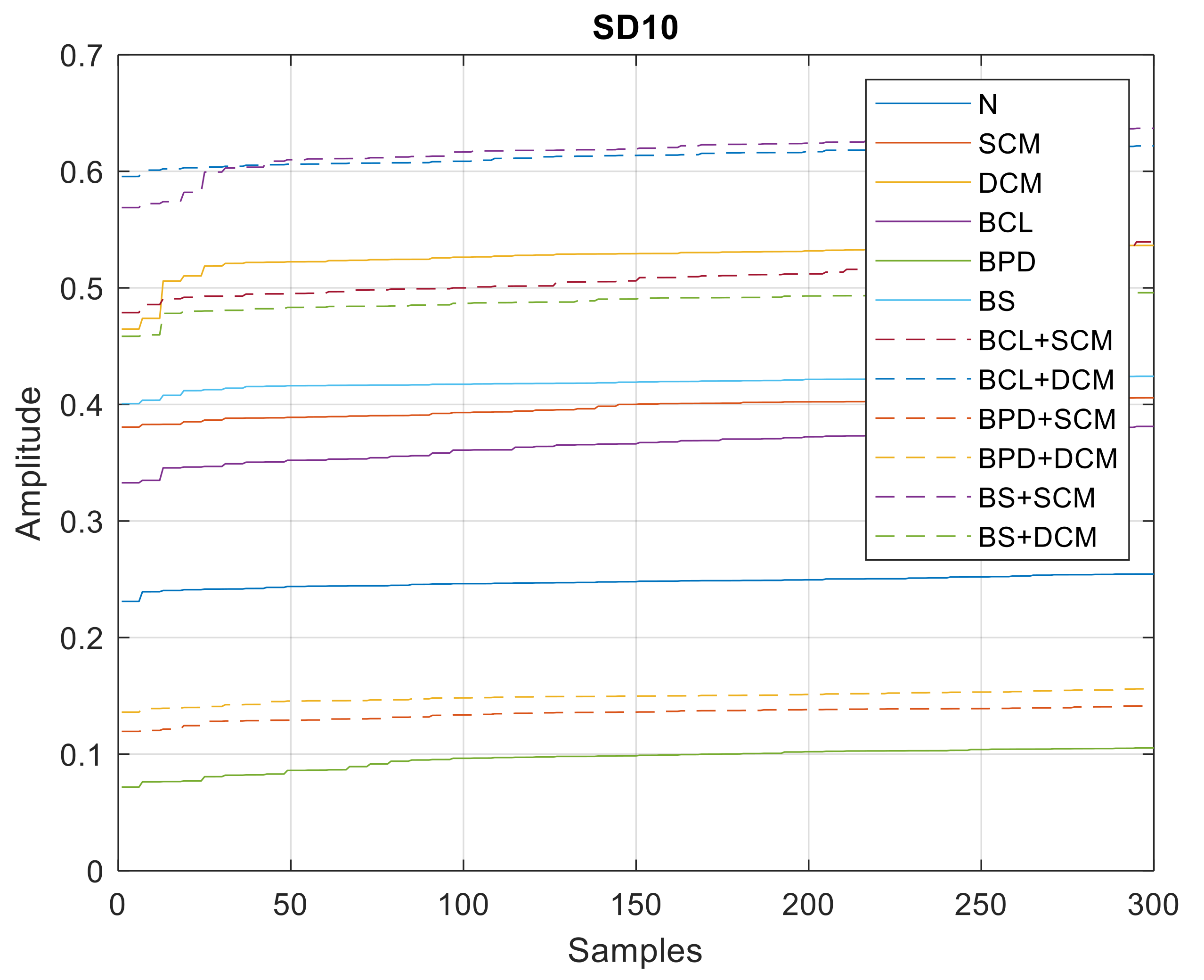
Figure 25.
SD10 values—single and double/simultaneous faults.
Figure 25.
SD10 values—single and double/simultaneous faults.
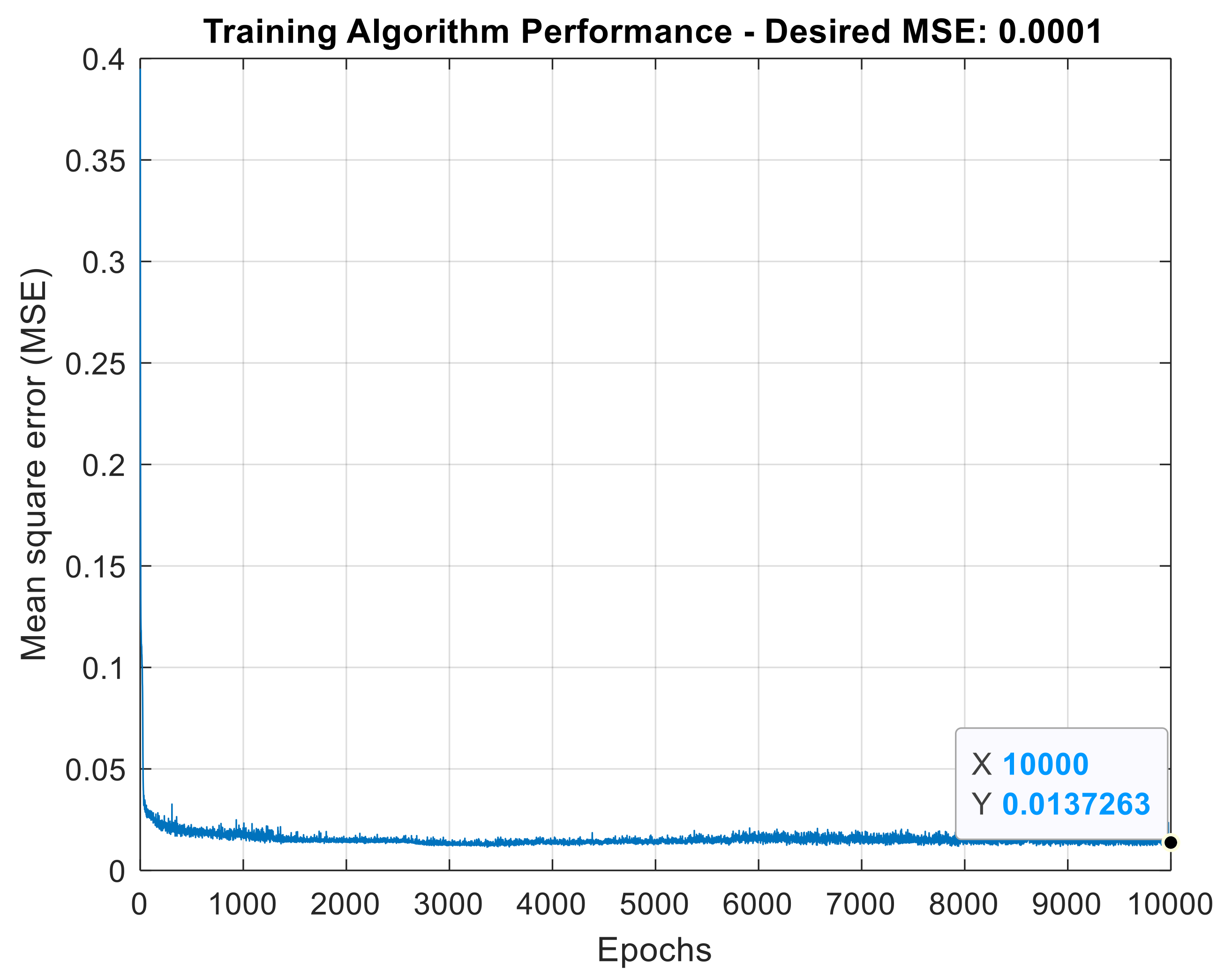
Figure 26.
ANN training algorithm performance for wavelet AMR-based strategy.
Figure 26.
ANN training algorithm performance for wavelet AMR-based strategy.
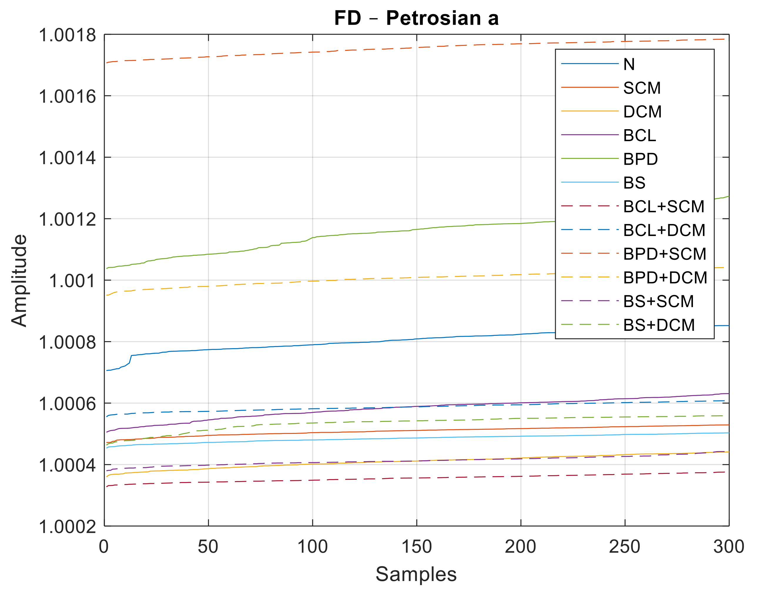
Figure 27.
FD values for the Petrosian a method.
Figure 27.
FD values for the Petrosian a method.
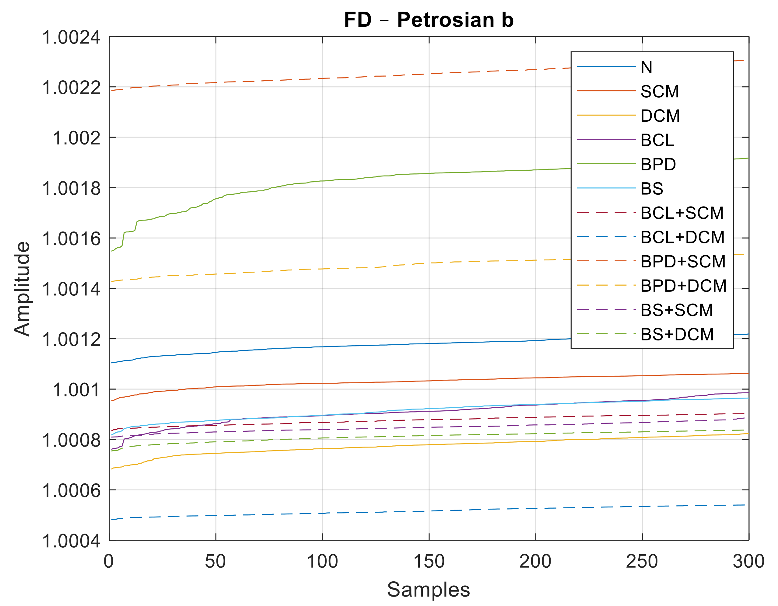
Figure 28.
FD values for the Petrosian b method.
Figure 28.
FD values for the Petrosian b method.
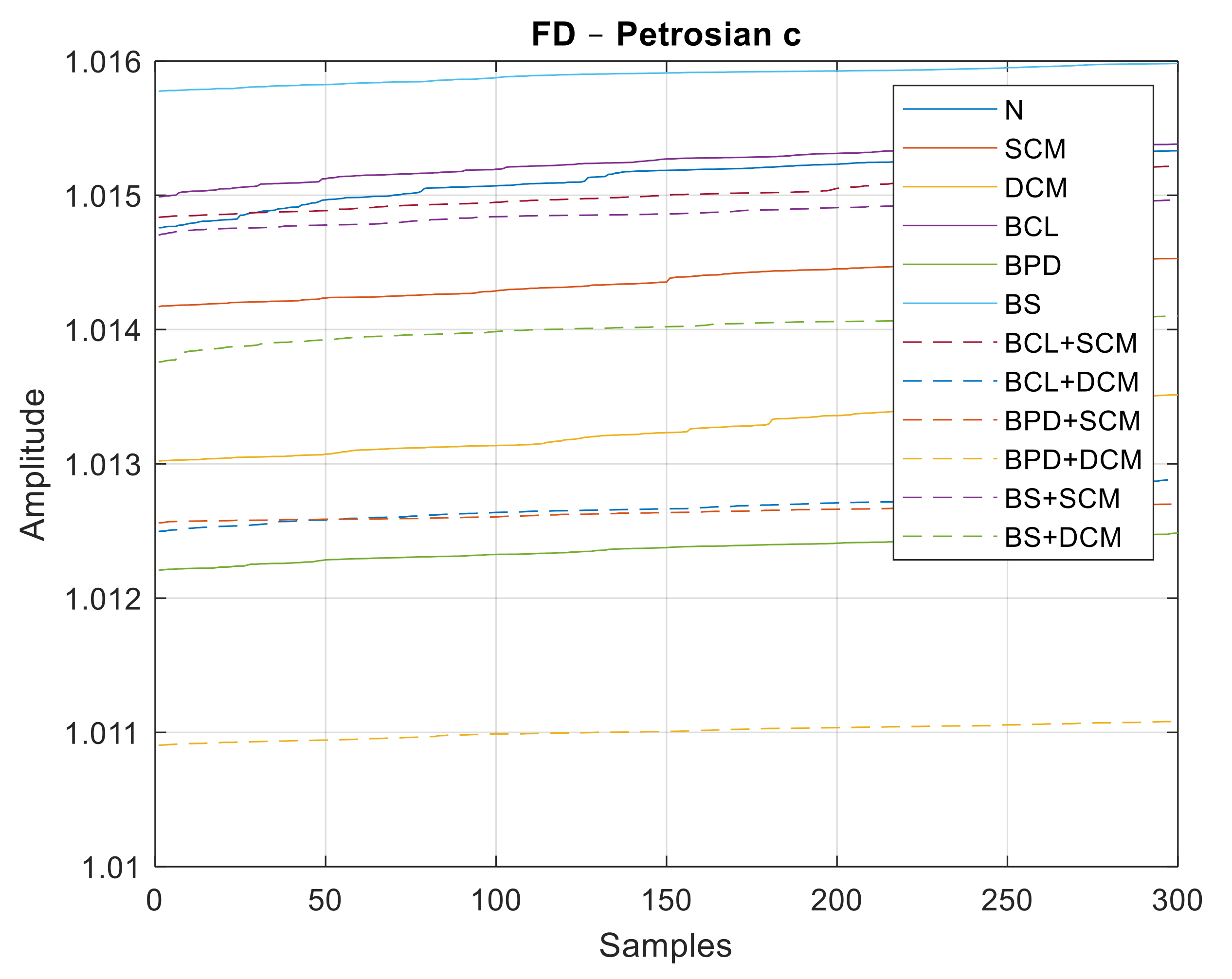
Figure 29.
FD values for the Petrosian c method.
Figure 29.
FD values for the Petrosian c method.
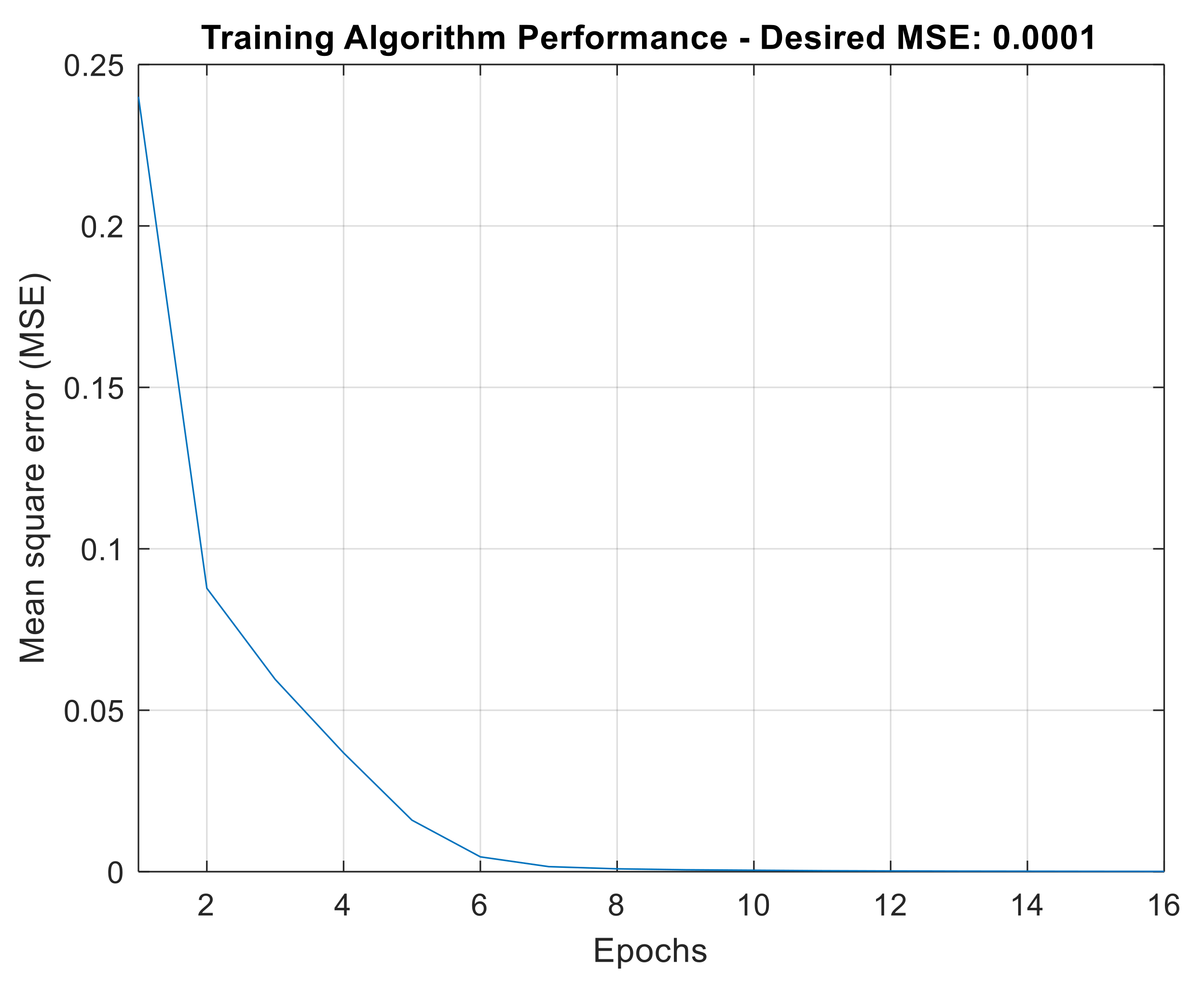
Figure 30.
ANN training algorithm performance for FD-based strategy.
Figure 30.
ANN training algorithm performance for FD-based strategy.
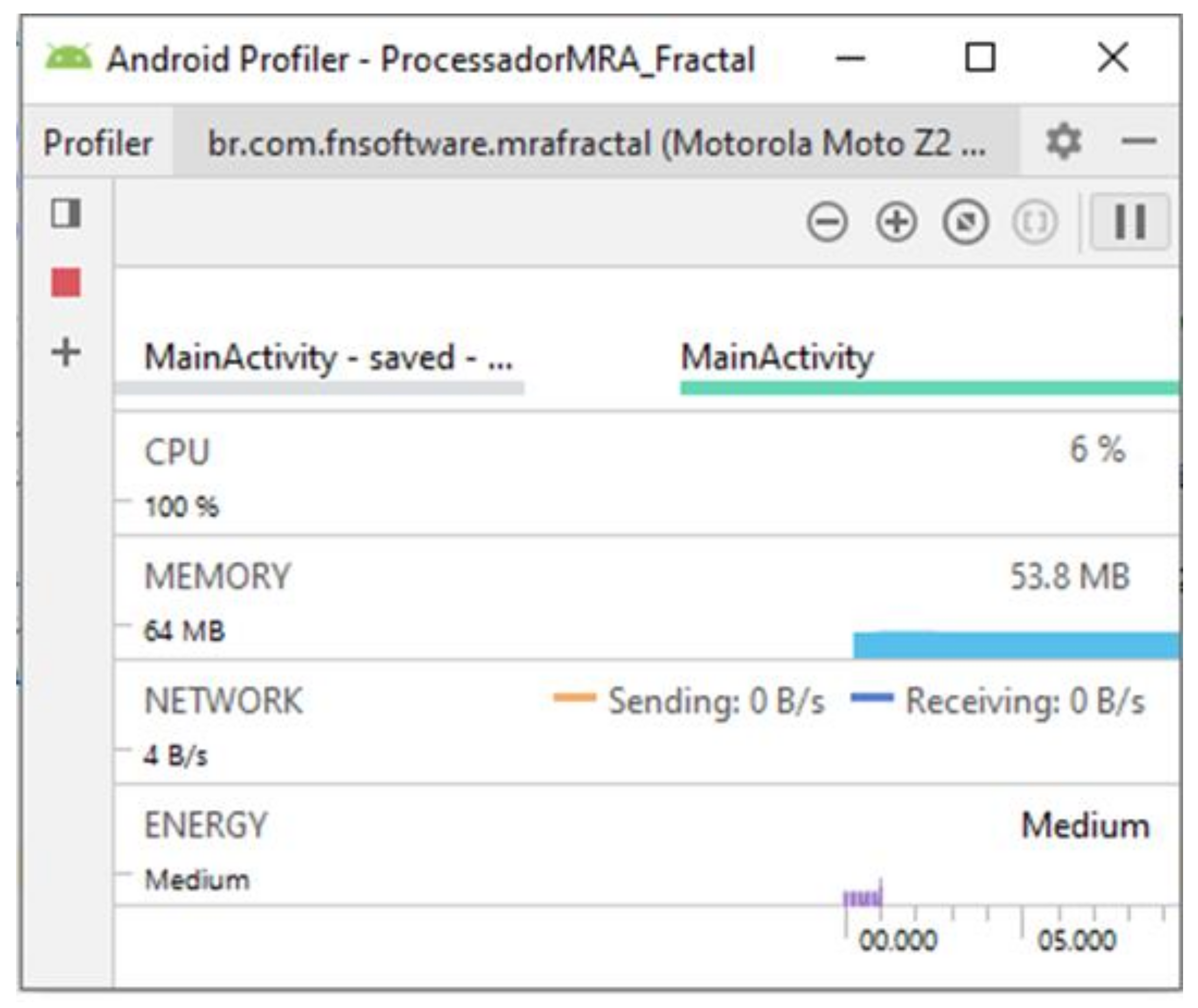
Figure 31.
Overall app performance—wavelet MRA-based strategy.
Figure 31.
Overall app performance—wavelet MRA-based strategy.
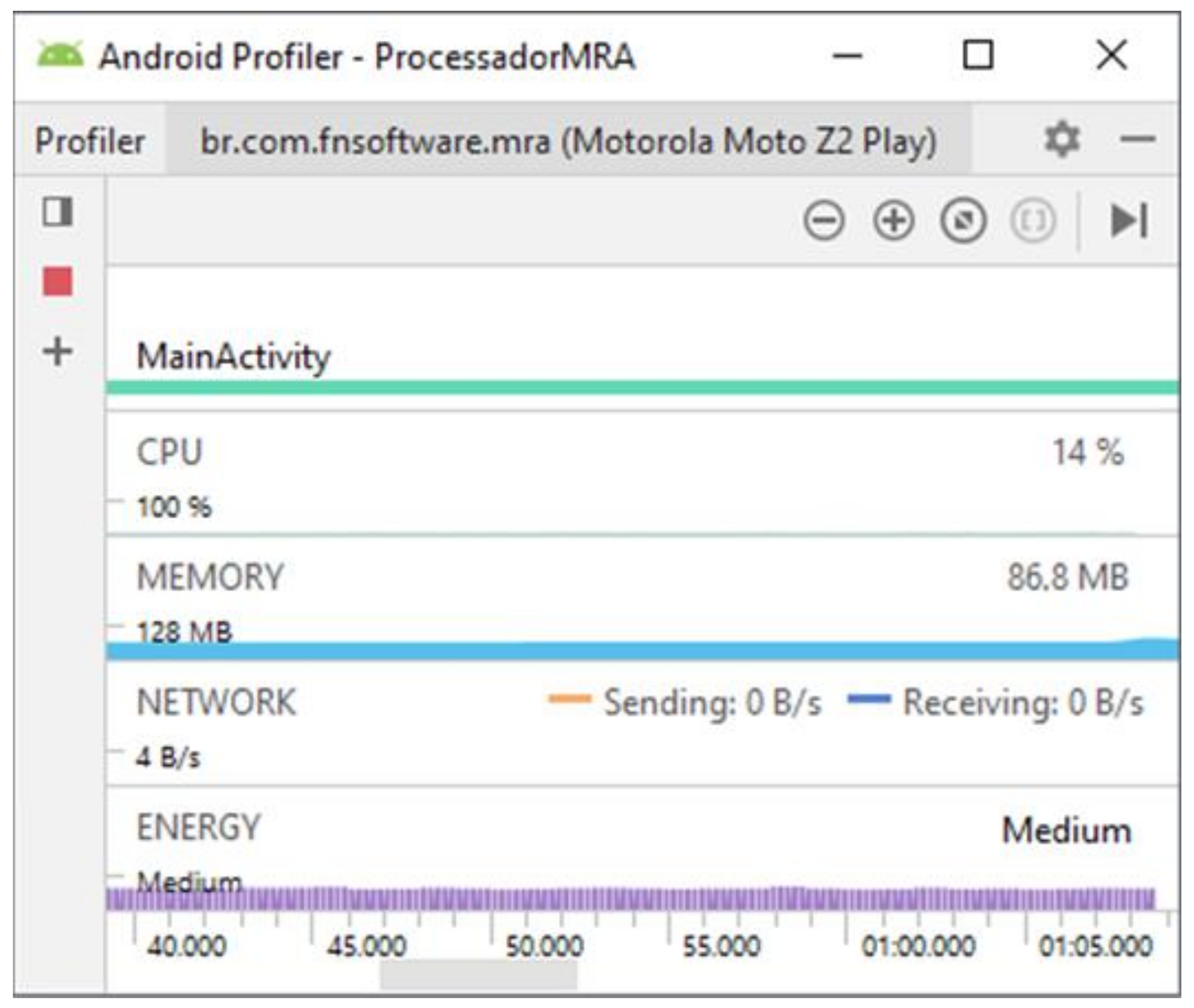
Figure 32.
Overall app performance—FD-based strategy.
Figure 32.
Overall app performance—FD-based strategy.
Table 1.
Range of frequency bands in wavelet decomposition.
Table 1.
Range of frequency bands in wavelet decomposition.
| Decomposed Signal | Frequency Range (Hz) |
|---|
| D1 | 11.025–22.050 |
| D2 | 5512.5–11.025 |
| D3 | 2756.25–5512.5 |
| D4 | 1378.12–2756.25 |
| D5 | 689.06–1378.12 |
| D6 | 344.53–689.06 |
| D7 | 172.26–344.53 |
| D8 | 86.13–172.26 |
| D9 | 43.06–86.13 |
| D10 | 21.53–43.06 |
Table 2.
Representation of fault classes.
Table 2.
Representation of fault classes.
| Neuron Outputs |
|---|
| Condition | N1 | N2 | N3 | N4 | N5 | N6 | N7 | N8 | N9 | N10 | N11 | N12 |
|---|
| Normal (N) | 1 | 0 | 0 | 0 | 0 | 0 | 0 | 0 | 0 | 0 | 0 | 0 |
| SCM | 0 | 1 | 0 | 0 | 0 | 0 | 0 | 0 | 0 | 0 | 0 | 0 |
| DCM | 0 | 0 | 1 | 0 | 0 | 0 | 0 | 0 | 0 | 0 | 0 | 0 |
| BPD | 0 | 0 | 0 | 1 | 0 | 0 | 0 | 0 | 0 | 0 | 0 | 0 |
| BCL | 0 | 0 | 0 | 0 | 1 | 0 | 0 | 0 | 0 | 0 | 0 | 0 |
| BS | 0 | 0 | 0 | 0 | 0 | 1 | 0 | 0 | 0 | 0 | 0 | 0 |
| BCL + SCM | 0 | 0 | 0 | 0 | 0 | 0 | 1 | 0 | 0 | 0 | 0 | 0 |
| BCL + DCM | 0 | 0 | 0 | 0 | 0 | 0 | 0 | 1 | 0 | 0 | 0 | 0 |
| BPD + SCM | 0 | 0 | 0 | 0 | 0 | 0 | 0 | 0 | 1 | 0 | 0 | 0 |
| BPD + DCM | 0 | 0 | 0 | 0 | 0 | 0 | 0 | 0 | 0 | 1 | 0 | 0 |
| BS + SCM | 0 | 0 | 0 | 0 | 0 | 0 | 0 | 0 | 0 | 0 | 1 | 0 |
| BS + DCM | 0 | 0 | 0 | 0 | 0 | 0 | 0 | 0 | 0 | 0 | 0 | 1 |
Table 3.
Signals used for validation of the acquisition system.
Table 3.
Signals used for validation of the acquisition system.
| Test Signal | Characteristic |
|---|
| Single tone—Sinusoidal | Fundamental Frequency = 1500 Hz |
| Two tones | F1 = 600 Hz/F2 = 1 kHz |
| AM signal | Carrier: 1 kHz/Modulator: 100 Hz |
Table 4.
Minimum, average and maximum values of the MRA parameters.
Table 4.
Minimum, average and maximum values of the MRA parameters.
| Parameters |
|---|
| | MD10 | SD10 | AD10 |
|---|
| Conditions | Min | Med | Max | Min | Med | Max | Min | Med | Max |
|---|
| Normal (N) | 0.19488 | 0.20876 | 0.21511 | 0.23106 | 0.24758 | 0.25454 | 0.05290 | 0.06073 | 0.06416 |
| SCM | 0.31622 | 0.33066 | 0.33831 | 0.38056 | 0.39690 | 0.40572 | 0.14341 | 0.15606 | 0.16299 |
| DCM | 0.40116 | 0.41845 | 0.42683 | 0.46469 | 0.52628 | 0.53641 | 0.26960 | 0.27919 | 0.28705 |
| BPD | 0.05792 | 0.07651 | 0.08451 | 0.07176 | 0.09593 | 0.10540 | 0.00510 | 0.00922 | 0.01101 |
| BCL | 0.27026 | 0.30302 | 0.31749 | 0.33278 | 0.36431 | 0.38114 | 0.10968 | 0.13159 | 0.14413 |
| BS | 0.35006 | 0.35731 | 0.36290 | 0.40071 | 0.41851 | 0.42416 | 0.16042 | 0.17358 | 0.17824 |
| BCL + SCM | 0.38449 | 0.42022 | 0.44873 | 0.47875 | 0.50758 | 0.53949 | 0.22694 | 0.25828 | 0.28879 |
| BCL + DCM | 0.46379 | 0.48876 | 0.50245 | 0.59556 | 0.61262 | 0.62177 | 0.35201 | 0.37393 | 0.38459 |
| BPD + SCM | 0.09333 | 0.10495 | 0.10989 | 0.11952 | 0.13464 | 0.14136 | 0.01423 | 0.01804 | 0.01979 |
| BPD + DCM | 0.10878 | 0.12028 | 0.12551 | 0.13605 | 0.14904 | 0.15606 | 0.01833 | 0.02230 | 0.02537 |
| BS + SCM | 0.43666 | 0.50717 | 0.52827 | 0.56887 | 0.61714 | 0.63686 | 0.32429 | 0.37767 | 0.40188 |
| BS + DCM | 0.37198 | 0.39480 | 0.40360 | 0.45845 | 0.48814 | 0.49585 | 0.20812 | 0.23606 | 0.24349 |
Table 5.
Confusion Matrix—wavelet MRA.
Table 5.
Confusion Matrix—wavelet MRA.
| Predicted Class | Target Class | Precision (%) |
|---|
| N | SCM | DCM | BPD | BCL | BS | BCL + SCM | BCL + DCM | BPD + SCM | BPD + DCM | BS + SCM | BS + DCM |
|---|
| Normal (N) | 120 | 0 | 0 | 0 | 0 | 0 | 0 | 0 | 0 | 0 | 0 | 0 | 100 |
| SCM | 0 | 117 | 0 | 0 | 1 | 0 | 0 | 0 | 0 | 0 | 0 | 0 | 99.15 |
| DCM | 0 | 0 | 120 | 0 | 0 | 0 | 0 | 0 | 0 | 0 | 0 | 0 | 100 |
| BPD | 0 | 0 | 0 | 120 | 0 | 0 | 0 | 0 | 0 | 0 | 0 | 0 | 100 |
| BCL | 0 | 3 | 0 | 0 | 119 | 0 | 0 | 0 | 0 | 0 | 0 | 0 | 97.54 |
| BS | 0 | 0 | 0 | 0 | 0 | 120 | 0 | 0 | 0 | 0 | 0 | 0 | 100 |
| BCL + SCM | 0 | 0 | 0 | 0 | 0 | 0 | 112 | 0 | 0 | 0 | 0 | 2 | 98.24 |
| BCL + DCM | 0 | 0 | 0 | 0 | 0 | 0 | 0 | 120 | 0 | 0 | 4 | 0 | 96.77 |
| BPD + SCM | 0 | 0 | 0 | 0 | 0 | 0 | 0 | 0 | 120 | 5 | 0 | 0 | 96 |
| BPD + DCM | 0 | 0 | 0 | 0 | 0 | 0 | 0 | 0 | 0 | 115 | 0 | 0 | 100 |
| BS + SCM | 0 | 0 | 0 | 0 | 0 | 0 | 0 | 0 | 0 | 0 | 116 | 0 | 100 |
| BS + DCM | 0 | 0 | 0 | 0 | 0 | 0 | 8 | 0 | 0 | 0 | 0 | 118 | 93.65 |
| Recall (%) | 100 | 97.50 | 100 | 100 | 99.16 | 100 | 93.33 | 100 | 100 | 95.83 | 96.66 | 98.33 | |
| | Accuracy (%) | 98.40 |
Table 6.
Minimum, average and maximum values of the FD extracted.
Table 6.
Minimum, average and maximum values of the FD extracted.
| Parameters |
|---|
| | FD—Petrosian a | FD—Petrosian b | FD—Petrosian c |
|---|
| Conditions | Min | Med | Max | Min | Med | Max | Min | Med | Max |
|---|
| Normal (N) | 1.00071 | 1.00080 | 1.00085 | 1.00110 | 1.00118 | 1.00122 | 1.01476 | 1.01513 | 1.01533 |
| SCM | 1.00047 | 1.00051 | 1.00053 | 1.00095 | 1.00103 | 1.00106 | 1.01417 | 1.01436 | 1.01453 |
| DCM | 1.00036 | 1.00041 | 1.00044 | 1.00068 | 1.00077 | 1.00082 | 1.01302 | 1.01325 | 1.01351 |
| BPD | 1.00103 | 1.00116 | 1.00127 | 1.00154 | 1.00183 | 1.00192 | 1.01221 | 1.01236 | 1.01248 |
| BCL | 1.00050 | 1.00058 | 1.00063 | 1.00076 | 1.00091 | 1.00099 | 1.01499 | 1.01524 | 1.01538 |
| BS | 1.00045 | 1.00049 | 1.00050 | 1.00082 | 1.00091 | 1.00096 | 1.01577 | 1.01589 | 1.01598 |
| BCL + SCM | 1.00032 | 1.00035 | 1.00038 | 1.00083 | 1.00088 | 1.00090 | 1.01483 | 1.01501 | 1.01522 |
| BCL + DCM | 1.00055 | 1.00059 | 1.00061 | 1.00048 | 1.00052 | 1.00054 | 1.01249 | 1.01268 | 1.01288 |
| BPD + SCM | 1.00171 | 1.00175 | 1.00178 | 1.00219 | 1.00225 | 1.00230 | 1.01256 | 1.01263 | 1.01270 |
| BPD + DCM | 1.00095 | 1.00100 | 1.00104 | 1.00143 | 1.00149 | 1.00153 | 1.01090 | 1.01100 | 1.01108 |
| BS + SCM | 1.00037 | 1.00041 | 1.00044 | 1.00080 | 1.00085 | 1.00089 | 1.01470 | 1.01486 | 1.01497 |
| BS + DCM | 1.00046 | 1.00053 | 1.00056 | 1.00075 | 1.00081 | 1.00083 | 1.01376 | 1.01401 | 1.01410 |
Table 7.
Confusion matrix—FD strategy.
Table 7.
Confusion matrix—FD strategy.
| Predicted Class | Target Class | Precision (%) |
|---|
| N | SCM | DCM | BPD | BCL | BS | BCL + SCM | BCL + DCM | BPD + SCM | BPD + DCM | BS + SCM | BS + DCM |
|---|
| Normal (N) | 120 | 0 | 0 | 0 | 0 | 0 | 0 | 0 | 0 | 0 | 0 | 0 | 100 |
| SCM | 0 | 118 | 0 | 0 | 3 | 0 | 0 | 0 | 0 | 0 | 0 | 0 | 97.52 |
| DCM | 0 | 0 | 120 | 0 | 0 | 0 | 0 | 0 | 0 | 0 | 0 | 0 | 100 |
| BPD | 0 | 0 | 0 | 120 | 0 | 0 | 0 | 0 | 0 | 0 | 0 | 0 | 100 |
| BCL | 0 | 1 | 0 | 0 | 117 | 0 | 0 | 0 | 0 | 0 | 0 | 0 | 99.15 |
| BS | 0 | 1 | 0 | 0 | 0 | 120 | 0 | 0 | 0 | 0 | 0 | 0 | 99.17 |
| BCL + SCM | 0 | 0 | 0 | 0 | 0 | 0 | 118 | 0 | 0 | 0 | 5 | 0 | 95.93 |
| BCL + DCM | 0 | 0 | 0 | 0 | 0 | 0 | 0 | 120 | 0 | 0 | 0 | 0 | 100 |
| BPD + SCM | 0 | 0 | 0 | 0 | 0 | 0 | 0 | 0 | 120 | 0 | 0 | 0 | 100 |
| BPD + DCM | 0 | 0 | 0 | 0 | 0 | 0 | 0 | 0 | 0 | 120 | 0 | 0 | 100 |
| BS + SCM | 0 | 0 | 0 | 0 | 0 | 0 | 2 | 0 | 0 | 0 | 115 | 0 | 98.29 |
| BS + DCM | 0 | 0 | 0 | 0 | 0 | 0 | 0 | 0 | 0 | 0 | 0 | 120 | 100 |
| Recall (%) | 100 | 98.33 | 100 | 100 | 97.50 | 100 | 98.33 | 100 | 100 | 100 | 95.83 | 100 | |
| | Accuracy (%) | 99.16 |


 ,
, 


