
Generating Images with Physics-Based Rendering for an Industrial Object Detection Task: Realism versus Domain Randomization


Abstract
:1. Introduction
- 1.
- We systematically generated multiple sets of PBR images with different levels of realism, used them to train an object detection model and evaluated the training images’ impact on average precision with real-world validation images.
- 2.
- Based on our results we provide guidelines for the generation of synthetic training images for industrial object detection tasks.
- 3.
- Our source code for generating training images with Blender is open source (https://github.com/ignc-research/blender-gen, accessed on 24 November 2021) and can be used for new industrial applications.
2. Related Work
2.1. Cut-and-Paste
2.2. Domain Randomization
2.3. Physics-Based Rendering
2.4. Domain Adaptation
2.5. Summary
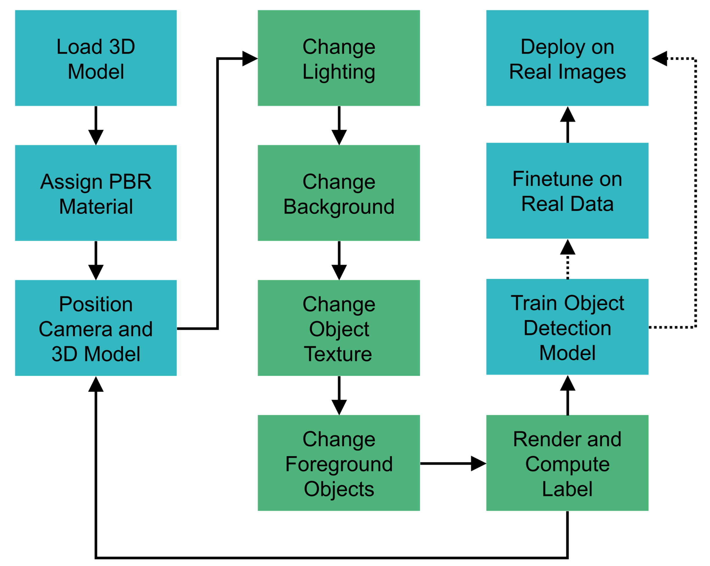
3. Method
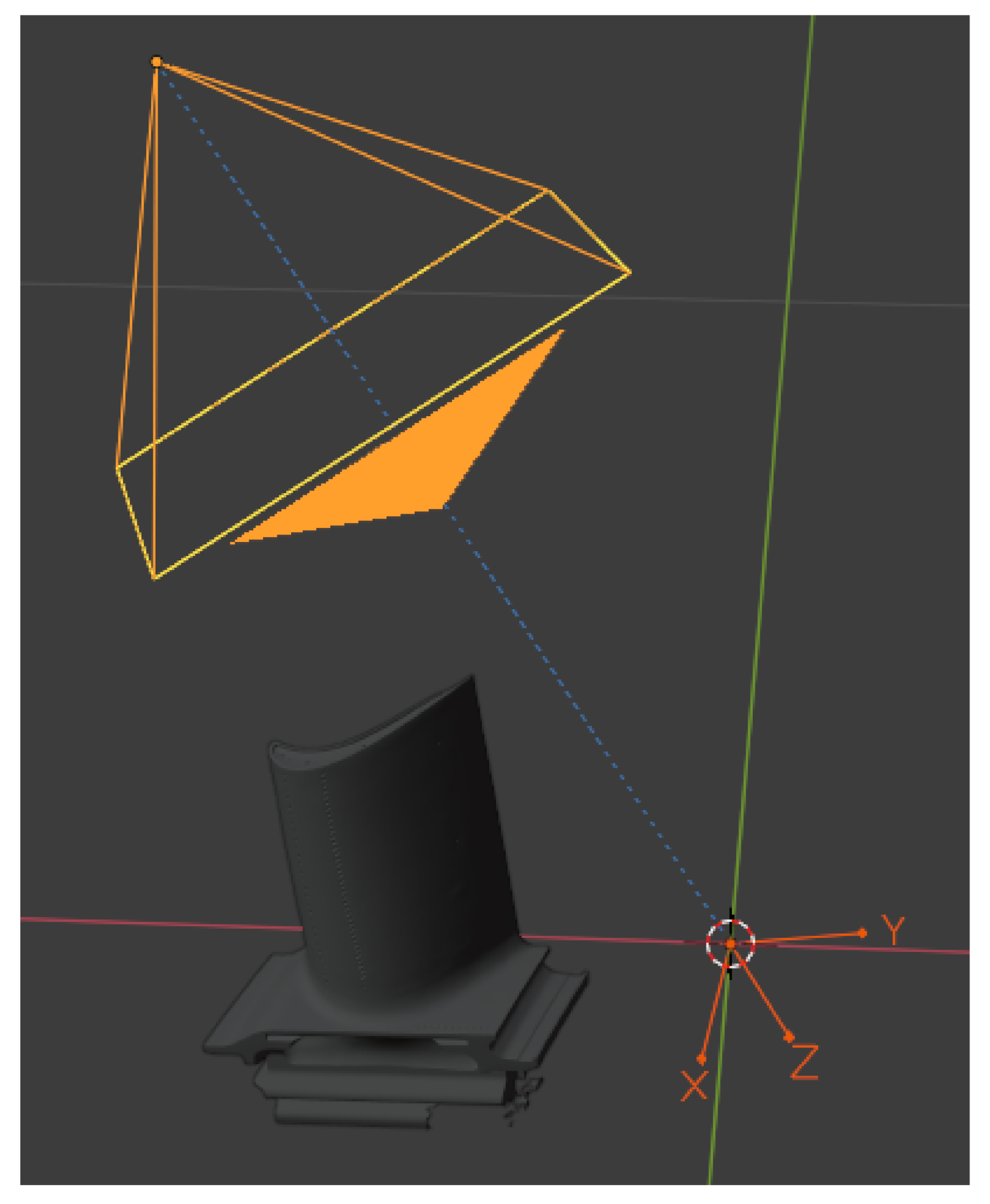
3.1. 3D Object Model
3.2. Positioning of Camera and 3D Object
3.3. Modeling of Lighting
3.3.1. Point Lights
3.3.2. Image-Based Lighting with HDRIs
3.4. Modeling of the Background
3.4.1. Random Background
3.4.2. HDRIs
3.4.3. Images of the Application Domain
3.5. Object Texture
3.6. Adding Foreground Objects
3.7. Computation of Bounding Box Labels
3.8. Object Detection Model and Training
3.9. Validation Data
4. Experiments and Results
4.1. Computation of the Bounding Box
4.2. Lighting
4.3. Background
4.4. Object Texture
4.5. Foreground Objects
4.6. Number of Rendered Images
4.7. Using Real Images
4.8. Transfer to New Objects
4.9. Qualitative Results
5. Discussion
6. Conclusions
Author Contributions
Funding
Institutional Review Board Statement
Informed Consent Statement
Data Availability Statement
Conflicts of Interest
Appendix A


References
- Nikolenko, S.I. Synthetic Data for Deep Learning. arXiv 2019, arXiv:1909.11512v1. [Google Scholar]
- Torralba, A.; Efros, A.A. Unbiased look at dataset bias. In Proceedings of the CVPR, Colorado Springs, CO, USA, 20–25 June 2011. [Google Scholar] [CrossRef] [Green Version]
- Movshovitz-Attias, Y.; Kanade, T.; Sheikh, Y. How Useful Is Photo-Realistic Rendering for Visual Learning? In Lecture Notes in Computer Science; Springer International Publishing: Cham, Switzerland, 2016; pp. 202–217. [Google Scholar] [CrossRef] [Green Version]
- Northcutt, C.G.; Jiang, L.; Chuang, I.L. Confident Learning: Estimating Uncertainty in Dataset Labels. arXiv 2021, arXiv:1911.00068v4. [Google Scholar] [CrossRef]
- Northcutt, C.G.; Athalye, A.; Mueller, J. Pervasive Label Errors in Test Sets Destabilize Machine Learning Benchmarks. arXiv 2021, arXiv:2103.14749v2. [Google Scholar]
- Schraml, D. Physically based synthetic image generation for machine learning: A review of pertinent literature. In Photonics and Education in Measurement Science; International Society for Optics and Photonics: Bellingham, WA, USA, 2019; Volume 11144. [Google Scholar] [CrossRef] [Green Version]
- Lambrecht, J.; Kästner, L. Towards the Usage of Synthetic Data for Marker-Less Pose Estimation of Articulated Robots in RGB Images. In Proceedings of the 2019 19th International Conference on Advanced Robotics (ICAR), Belo Horizonte, Brazil, 2–6 December 2019. [Google Scholar] [CrossRef]
- Nowruzi, F.E.; Kapoor, P.; Kolhatkar, D.; Hassanat, F.A.; Laganiere, R.; Rebut, J. How much real data do we actually need: Analyzing object detection performance using synthetic and real data. arXiv 2019, arXiv:1907.07061v1. [Google Scholar]
- Candela, J. Dataset Shift in Machine Learning; MIT Press: Cambridge, MA, USA; London, UK, 2009. [Google Scholar]
- Dwibedi, D.; Misra, I.; Hebert, M. Cut, Paste and Learn: Surprisingly Easy Synthesis for Instance Detection. In Proceedings of the 2017 IEEE International Conference on Computer Vision (ICCV), Venice, Italy, 22–29 October 2017. [Google Scholar] [CrossRef] [Green Version]
- Tremblay, J.; Prakash, A.; Acuna, D.; Brophy, M.; Jampani, V.; Anil, C.; To, T.; Cameracci, E.; Boochoon, S.; Birchfield, S. Training Deep Networks with Synthetic Data: Bridging the Reality Gap by Domain Randomization. In Proceedings of the 2018 IEEE/CVF Conference on Computer Vision and Pattern Recognition Workshops (CVPRW), Salt Lake City, UT, USA, 18–22 June 2018. [Google Scholar] [CrossRef] [Green Version]
- Hodan, T.; Vineet, V.; Gal, R.; Shalev, E.; Hanzelka, J.; Connell, T.; Urbina, P.; Sinha, S.N.; Guenter, B. Photorealistic Image Synthesis for Object Instance Detection. In Proceedings of the 2019 IEEE International Conference on Image Processing (ICIP), Taipei, Taiwan, 22–25 September 2019. [Google Scholar] [CrossRef] [Green Version]
- Mayer, N.; Ilg, E.; Fischer, P.; Hazirbas, C.; Cremers, D.; Dosovitskiy, A.; Brox, T. What Makes Good Synthetic Training Data for Learning Disparity and Optical Flow Estimation? Int. J. Comput. Vis. 2018, 126, 942–960. [Google Scholar] [CrossRef] [Green Version]
- Everingham, M.; Eslami, S.M.A.; Van Gool, L.; Williams, C.K.I.; Winn, J.; Zisserman, A. The Pascal Visual Object Classes Challenge: A Retrospective. Int. J. Comput. Vis. 2015, 111, 98–136. [Google Scholar] [CrossRef]
- Lin, T.Y.; Maire, M.; Belongie, S.; Hays, J.; Perona, P.; Ramanan, D.; Dollár, P.; Zitnick, C.L. Microsoft COCO: Common Objects in Context. In Computer Vision — ECCV 2014; Springer International Publishing: Cham, Switzerland, 2014; pp. 740–755. [Google Scholar] [CrossRef] [Green Version]
- Pharr, M.; Jakob, W.; Humphreys, G. Physically Based Rendering: From Theory to Implementation, 3rd ed.; Morgan Kaufmann: Burlington, MA, USA, 2016. [Google Scholar]
- Georgakis, G.; Mousavian, A.; Berg, A.; Kosecka, J. Synthesizing Training Data for Object Detection in Indoor Scenes. In Proceedings of the Robotics: Science and Systems XIII, Robotics: Science and Systems Foundation, Cambridge, MA, USA, 12–16 July 2017. [Google Scholar] [CrossRef]
- Georgakis, G.; Reza, M.A.; Mousavian, A.; Le, P.H.; Kosecka, J. Multiview RGB-D Dataset for Object Instance Detection. In Proceedings of the IEEE 2016 Fourth International Conference on 3D Vision (3DV), Stanford, CA, USA, 25–28 October 2016. [Google Scholar] [CrossRef] [Green Version]
- Dvornik, N.; Mairal, J.; Schmid, C. Modeling Visual Context Is Key to Augmenting Object Detection Datasets. In Computer Vision—ECCV 2018; Springer International Publishing: Cham, Switzerland, 2018; pp. 375–391. [Google Scholar] [CrossRef] [Green Version]
- Tobin, J.; Fong, R.; Ray, A.; Schneider, J.; Zaremba, W.; Abbeel, P. Domain randomization for transferring deep neural networks from simulation to the real world. In Proceedings of the 2017 IEEE/RSJ International Conference on Intelligent Robots and Systems (IROS), Vancouver, BC, Canada, 24–28 September 2017. [Google Scholar] [CrossRef] [Green Version]
- Prakash, A.; Boochoon, S.; Brophy, M.; Acuna, D.; Cameracci, E.; State, G.; Shapira, O.; Birchfield, S. Structured Domain Randomization: Bridging the Reality Gap by Context-Aware Synthetic Data. In Proceedings of the IEEE 2019 International Conference on Robotics and Automation (ICRA), Montreal, QC, Canada, 20–24 May 2019. [Google Scholar] [CrossRef] [Green Version]
- Hinterstoisser, S.; Lepetit, V.; Wohlhart, P.; Konolige, K. On Pre-Trained Image Features and Synthetic Images for Deep Learning. In Computer Vision—ECCV 2018 Workshops; Springer International Publishing: Cham, Switzerland, 2017; pp. 682–697. [Google Scholar] [CrossRef] [Green Version]
- Phong, B.T. Illumination for Computer Generated Pictures. Commun. ACM 1975, 18, 311–317. [Google Scholar] [CrossRef] [Green Version]
- Hinterstoisser, S.; Pauly, O.; Heibel, H.; Marek, M.; Bokeloh, M. An Annotation Saved is an Annotation Earned: Using Fully Synthetic Training for Object Instance Detection. In Proceedings of the 2019 IEEE/CVF International Conference on Computer Vision Workshop (ICCVW), Seoul, Korea, 27–28 October 2019; pp. 2787–2796. [Google Scholar] [CrossRef]
- Tsirikoglou, A.; Eilertsen, G.; Unger, J. A Survey of Image Synthesis Methods for Visual Machine Learning. Comput. Graph. Forum 2020, 39, 426–451. [Google Scholar] [CrossRef]
- Georgiev, I.; Ize, T.; Farnsworth, M.; Montoya-Vozmediano, R.; King, A.; Lommel, B.V.; Jimenez, A.; Anson, O.; Ogaki, S.; Johnston, E.; et al. Arnold: A Brute-Force Production Path Tracer. ACM Trans. Graph. 2018, 37, 1–12. [Google Scholar] [CrossRef]
- Hinterstoisser, S.; Lepetit, V.; Ilic, S.; Holzer, S.; Bradski, G.; Konolige, K.; Navab, N. Model Based Training, Detection and Pose Estimation of Texture-Less 3D Objects in Heavily Cluttered Scenes. In Computer Vision — ACCV 2012; Springer: Berlin/Heidelberg, Germany, 2013; pp. 548–562. [Google Scholar] [CrossRef] [Green Version]
- Brachmann, E.; Krull, A.; Michel, F.; Gumhold, S.; Shotton, J.; Rother, C. Learning 6D Object Pose Estimation Using 3D Object Coordinates. In Computer Vision—ECCV 2014; Springer International Publishing: Cham, Switzerland, 2014; pp. 536–551. [Google Scholar] [CrossRef] [Green Version]
- Rennie, C.; Shome, R.; Bekris, K.E.; Souza, A.F.D. A Dataset for Improved RGBD-Based Object Detection and Pose Estimation for Warehouse Pick-and-Place. IEEE Robot. Autom. Lett. 2016, 1, 1179–1185. [Google Scholar] [CrossRef] [Green Version]
- Rudorfer, M.; Neumann, L.; Kruger, J. Towards Learning 3d Object Detection and 6d Pose Estimation from Synthetic Data. In Proceedings of the 2019 24th IEEE International Conference on Emerging Technologies and Factory Automation (ETFA), Zaragoza, Spain, 10–13 September 2019. [Google Scholar] [CrossRef]
- Tekin, B.; Sinha, S.N.; Fua, P. Real-Time Seamless Single Shot 6D Object Pose Prediction. In Proceedings of the 2018 IEEE/CVF Conference on Computer Vision and Pattern Recognition, Salt Lake City, UT, USA, 18–22 June 2018. [Google Scholar] [CrossRef] [Green Version]
- Jabbar, A.; Farrawell, L.; Fountain, J.; Chalup, S.K. Training Deep Neural Networks for Detecting Drinking Glasses Using Synthetic Images. In Neural Information Processing; Springer International Publishing: Cham, Switzerland, 2017; pp. 354–363. [Google Scholar] [CrossRef]
- Reinhard, E.; Heidrich, W.; Debevec, P.; Pattanaik, S.; Ward, G.; Myszkowski, K. High Dynamic Range Imaging: Acquisition, Display, and Image-Based Lighting; Morgan Kaufmann: Burlington, MA, USA, 2010. [Google Scholar]
- Wong, M.Z.; Kunii, K.; Baylis, M.; Ong, W.H.; Kroupa, P.; Koller, S. Synthetic dataset generation for object-to-model deep learning in industrial applications. PeerJ Comput. Sci. 2019, 5, e222. [Google Scholar] [CrossRef] [PubMed] [Green Version]
- Xiao, J.; Hays, J.; Ehinger, K.A.; Oliva, A.; Torralba, A. SUN database: Large-scale scene recognition from abbey to zoo. In Proceedings of the 2010 IEEE Computer Society Conference on Computer Vision and Pattern Recognition, San Francisco, CA, USA, 13–18 June 2010. [Google Scholar] [CrossRef]
- Goodfellow, I.; Pouget-Abadie, J.; Mirza, M.; Xu, B.; Warde-Farley, D.; Ozair, S.; Courville, A.; Bengio, Y. Generative adversarial nets. In Advances in Neural Information Processing Systems; MIT Press: Cambridge, MA, USA, 2014; Volume 27. [Google Scholar]
- Shrivastava, A.; Pfister, T.; Tuzel, O.; Susskind, J.; Wang, W.; Webb, R. Learning From Simulated and Unsupervised Images Through Adversarial Training. In Proceedings of the IEEE Conference on Computer Vision and Pattern Recognition (CVPR), Honolulu, HI, USA, 21–26 July 2017. [Google Scholar]
- Peng, X.; Saenko, K. Synthetic to Real Adaptation with Generative Correlation Alignment Networks. In Proceedings of the 2018 IEEE Winter Conference on Applications of Computer Vision (WACV), Lake Tahoe, NV, USA, 12–15 March 2018. [Google Scholar] [CrossRef] [Green Version]
- Sankaranarayanan, S.; Balaji, Y.; Jain, A.; Lim, S.N.; Chellappa, R. Learning From Synthetic Data: Addressing Domain Shift for Semantic Segmentation. In Proceedings of the IEEE Conference on Computer Vision and Pattern Recognition (CVPR), Salt Lake City, UT, USA, 18–22 June 2018. [Google Scholar]
- Rojtberg, P.; Pollabauer, T.; Kuijper, A. Style-transfer GANs for bridging the domain gap in synthetic pose estimator training. In Proceedings of the 2020 IEEE International Conference on Artificial Intelligence and Virtual Reality (AIVR), Utrecht, The Netherlands, 14–18 December 2020. [Google Scholar] [CrossRef]
- Su, Y.; Rambach, J.; Pagani, A.; Stricker, D. SynPo-Net—Accurate and Fast CNN-Based 6DoF Object Pose Estimation Using Synthetic Training. Sensors 2021, 21, 300. [Google Scholar] [CrossRef] [PubMed]
- Rambach, J.; Deng, C.; Pagani, A.; Stricker, D. Learning 6DoF Object Poses from Synthetic Single Channel Images. In Proceedings of the 2018 IEEE International Symposium on Mixed and Augmented Reality Adjunct (ISMAR-Adjunct), Munich, Germany, 16–20 October 2018. [Google Scholar] [CrossRef]
- Hodosh, M.; Young, P.; Hockenmaier, J. Framing image description as a ranking task: Data, models and evaluation metrics. J. Artif. Intell. Res. 2013, 47, 853–899. [Google Scholar] [CrossRef] [Green Version]
- Andulkar, M.; Hodapp, J.; Reichling, T.; Reichenbach, M.; Berger, U. Training CNNs from Synthetic Data for Part Handling in Industrial Environments. In Proceedings of the 2018 IEEE 14th International Conference on Automation Science and Engineering (CASE), Munich, Germany, 20–24 August 2018. [Google Scholar] [CrossRef]
- Denninger, M.; Sundermeyer, M.; Winkelbauer, D.; Olefir, D.; Hodan, T.; Zidan, Y.; Elbadrawy, M.; Knauer, M.; Katam, H.; Lodhi, A. BlenderProc: Reducing the Reality Gap with Photorealistic Rendering. In Proceedings of the Robotics: Science and Systems (RSS), Virtual Event/Corvalis, OR, USA, 12–16 July 2020. [Google Scholar]
- Hodan, T.; Haluza, P.; Obdrzalek, S.; Matas, J.; Lourakis, M.; Zabulis, X. T-LESS: An RGB-D Dataset for 6D Pose Estimation of Texture-Less Objects. In Proceedings of the 2017 IEEE Winter Conference on Applications of Computer Vision (WACV), Santa Rosa, CA, USA, 24–31 March 2017; pp. 880–888. [Google Scholar] [CrossRef] [Green Version]
- Drost, B.; Ulrich, M.; Bergmann, P.; Härtinger, P.; Steger, C. Introducing MVTec ITODD—A Dataset for 3D Object Recognition in Industry. In Proceedings of the 2017 IEEE International Conference on Computer Vision Workshops (ICCVW), Venice, Italy, 22–29 October 2017; pp. 2200–2208. [Google Scholar] [CrossRef]
- ISO 3664:2009. In Graphic Technology and Photography—Viewing Conditions; International Organization for Standardization: Geneva, Switzerland, 2009.
- Charity, M. What Color Is a Blackbody?—Some Pixel Rgb Values. Available online: http://www.vendian.org/mncharity/dir3/blackbody/ (accessed on 9 April 2019).
- Calli, B.; Singh, A.; Walsman, A.; Srinivasa, S.; Abbeel, P.; Dollar, A.M. The YCB object and Model set: Towards common benchmarks for manipulation research. In Proceedings of the 2015 International Conference on Advanced Robotics (ICAR), Istanbul, Turkey, 27–31 July 2015. [Google Scholar] [CrossRef]
- Ren, S.; He, K.; Girshick, R.; Sun, J. Faster R-CNN: Towards Real-Time Object Detection with Region Proposal Networks. In Advances in Neural Information Processing Systems; MIT Press: Cambridge, MA, USA, 2015; Volume 28, pp. 91–99. [Google Scholar]
- He, K.; Zhang, X.; Ren, S.; Sun, J. Deep Residual Learning for Image Recognition. In Proceedings of the 2016 IEEE Conference on Computer Vision and Pattern Recognition (CVPR), Las Vegas, NV, USA, 27–30 June 2016. [Google Scholar] [CrossRef] [Green Version]
- Girshick, R. Fast R-CNN. In Proceedings of the IEEE International Conference on Computer Vision (ICCV), Santiago, Chile, 7–13 December 2015. [Google Scholar]
- Everingham, M.; Gool, L.V.; Williams, C.K.I.; Winn, J.; Zisserman, A. The Pascal Visual Object Classes (VOC) Challenge. Int. J. Comput. Vis. 2009, 88, 303–338. [Google Scholar] [CrossRef] [Green Version]
- Goodfellow, I.; Bengio, Y.; Courville, A. Deep Learning; MIT Press: Cambridge, MA, USA; London, UK, 2016. [Google Scholar]


| Lighting | Background | Object Texture | Occlusion | Object Placement | |
|---|---|---|---|---|---|
Hodaň et al. [12]  | Standard light sources (e.g., point lights) and Arnold Physical Sky [26] | 3D scene models | From 3D model | Multiple 3D objects | Physics simulation |
Rudorfer et al. [30]  | White point lights | Application domain images or COCO | From 3D model | Multiple 3D objects | Random |
Movshovitz-Attias et al. [3]  | Directed light w/ different light temperatures | PASCAL | From 3D model | Rectangular patches | Random |
Jabbar et al. [32]  | IBL from HDRIs | 360° HDRIs | Glass material | None | On a flat surface |
Wong et al. [34]  | White point lights | SUN | From 3D model | None | Random |
Tremblay et al. [11]  | White point lights and planar light | Flickr 8K [43] | Random (Flickr 8K) | Multiple 3D geometric shapes | On a ground plane |
Hinterstoisser et al. [22,24]  | Random phong light with random light color | Application domain images or random 3D models | From 3D model | None or multiple 3D objects | Random |
| Hyperparameter | Value |
|---|---|
| Optimizer [55] | Stochastic gradient descent (SGD) with learning rate , momentum , L2 weight decay |
| Epochs | 25 |
| Training examples | 5000 |
| Batch size | 8 |
| Image size | 640 pixel × 360 pixel |
| Lighting Model | E | |||
|---|---|---|---|---|
| PL (white) | 0.623 | 0.917 | ||
| PL (white) | 0.633 | 0.908 | ||
| PL (white) | 0.632 | 0.919 | ||
| PL (white) | 0.633 | 0.914 | ||
| PL (white) | 0.631 | 0.928 | ||
| PL (temperature) | 0.635 | 0.929 | ||
| IBL with HDRIs | - | 0.640 | 0.926 | |
| IBL with HDRIs | - | 0.642 | 0.926 | |
| IBL with HDRIs | - | 0.641 | 0.931 | |
| IBL with HDRIs | - | 0.642 | 0.931 |
| Background Model | ||
|---|---|---|
| COCO images | 0.642 | 0.931 |
| HDRI images | 0.589 | 0.899 |
| Deployment domain images | 0.612 | 0.938 |
| 50% COCO and 50% deployment images | 0.635 | 0.935 |
| 75% COCO and 25% deployment images | 0.634 | 0.925 |
| 90% COCO and 10% deployment images | 0.641 | 0.931 |
| Texture Model | ||
|---|---|---|
| Grey base color | 0.642 | 0.931 |
| Random COCO images | 0.623 | 0.946 |
| Random material texture | 0.644 | 0.962 |
| Realistic material texture | 0.653 | 0.963 |
| Real material texture | 0.648 | 0.948 |
| Foreground Objects | Texture | |||
|---|---|---|---|---|
| None | 0 | - | 0.653 | 0.963 |
| YCB tools | Original | 0.657 | 0.963 | |
| YCB tools | Original | 0.653 | 0.963 | |
| YCB tools | Original | 0.660 | 0.972 | |
| YCB tools | Original | 0.659 | 0.972 | |
| YCB tools | COCO | 0.653 | 0.951 | |
| YCB tools | Random material | 0.647 | 0.958 | |
| Cubes | COCO | 0.666 | 0.987 | |
| Cubes | Random material | 0.669 | 0.989 |
| Model | |||
|---|---|---|---|
| Real training images | 200 | 0.709 | 0.985 |
| PBR training images | 5000 | 0.704 | 0.989 |
| Pre-trained on PBR and fine-tuned on real images | 5000 and 200 | 0.785 | 1.00 |
| Object | Baseline | IBL with HDRIs | Realistic Material Texture | Foreground Objects |
|---|---|---|---|---|
| TB 1 | 0.620 | 0.662 | 0.663 | 0.677 |
| TB 2 | 0.481 | 0.568 | 0.580 | 0.629 |
| TB 3 | 0.466 | 0.467 | 0.501 | 0.556 |
| mean | 0.522 | 0.566 | 0.581 | 0.621 |
Publisher’s Note: MDPI stays neutral with regard to jurisdictional claims in published maps and institutional affiliations. |
© 2021 by the authors. Licensee MDPI, Basel, Switzerland. This article is an open access article distributed under the terms and conditions of the Creative Commons Attribution (CC BY) license (https://creativecommons.org/licenses/by/4.0/).
Share and Cite
Eversberg, L.; Lambrecht, J. Generating Images with Physics-Based Rendering for an Industrial Object Detection Task: Realism versus Domain Randomization. Sensors 2021, 21, 7901. https://doi.org/10.3390/s21237901
Eversberg L, Lambrecht J. Generating Images with Physics-Based Rendering for an Industrial Object Detection Task: Realism versus Domain Randomization. Sensors. 2021; 21(23):7901. https://doi.org/10.3390/s21237901
Chicago/Turabian StyleEversberg, Leon, and Jens Lambrecht. 2021. "Generating Images with Physics-Based Rendering for an Industrial Object Detection Task: Realism versus Domain Randomization" Sensors 21, no. 23: 7901. https://doi.org/10.3390/s21237901
APA StyleEversberg, L., & Lambrecht, J. (2021). Generating Images with Physics-Based Rendering for an Industrial Object Detection Task: Realism versus Domain Randomization. Sensors, 21(23), 7901. https://doi.org/10.3390/s21237901