1. Introduction
Data fusion is a mathematical discipline that deals with the acquisition, processing, and combination of synergies of information gathered from sensors [
1]. Data fusion can be defined as the combination of data and information from different sources, to obtain improved information [
2]. This data fusion is usually done to analyze and understand a phenomenon [
3,
4,
5], for instance a system malfunction. Data fusion techniques are present in a wide range of applications, such as smart city applications [
6], allowing to manage multiple data sources; food analysis context [
7]; guidance and control of autonomous vehicles [
8]; medical studies [
9], and so on. In addition, there are different analysis methods that combine data from different sources, where the most common options are algorithms based on optimization [
10], multiblock (or multitable) methods [
11], and statistical data fusion [
12]. In our article, we used an original statistical parametric identification to perform data fusion, where covariance of sensory information is not required, which is generally not available.
Moreover, the data sensor has been useful to detect possible failures in the pitch actuator systems of wind turbines [
13,
14,
15,
16]. Furthermore, it turns out that a parameterized plant modeling can be a key factor for efficient fault diagnosis based on the fusion of sensor data. If in addition, only a single sensor is used for the data fusion process, an option to generate data to be merged is through an iterative process. On the other hand, it is well known that the iterative learning process can improve your performance on repetitive tasks in a finite period of time [
17,
18,
19]. Therefore, the main objective of this article is to develop a fusion of a sensor data based on adaptive iterative learning. This process will provide data in each periodic cycle task that will be further analyzed for fault diagnosis in the wind turbine pitch actuators.
The pitch system of a wind turbine adjusts the pitch angle of the blade by turning it. In the case of a three-bladed wind turbine, there are generally three identical pitch actuators [
15,
20]. This part of a wind turbine is responsible for capturing the wind to convert it into mechanical energy and then into electrical one. Therefore, if the pitch actuator system has a fault, the energy efficiency conversion will be affected, among others mechanical and structural wear. Some common faults are high oil content in the air, hydraulic leaks, and pump wear. Our data fusion approach is capable of detecting these types of failures.
The iterative learning theory used for adaptive learning of a process is a key factor in many iterative learning control frameworks [
17,
18,
19]. Therefore, an appropriate mathematical model of the pitch system will be important, and as simple as possible to perform a simple adaptive iterative learning method to our main objective. Furthermore, an iterative learning control has been used to improve control performance of proportional controllers and derivative ones [
21]. Simulation results are given in [
21] to support this affirmation. In [
22], an iterative learning control theory is employed in a first-order hyperbolic system that helps improve controller robustness on desired time-varying trajectories. This is also supported by performing numerical examples of given hyperbolic systems. In addition, [
23] shows the realization of the synchronization of non-identical neural network systems that have a variable delay in time coupled by means of an iterative learning control. According to the simulation results shown in [
23], the synchronization objective is satisfied. Finally, in [
24], iterative learning control is applied to a novel computational fluid dynamics model to show the performance of the controller in improving the aerodynamic load of wind turbines. In the same way, we will use numerical results to support our main contribution.
The rest of the structure of this article is as follows.
Section 2 presents our data fusion approach by using a simple mathematical model of the pitch system, and the use of an adaptive iterative learning framework based on Lyapunov’s theory.
Section 3 shows the results of numerical simulations and followed by
Section 4, where the advantages of the proposed method are discussed. Finally, a summary is presented in
Section 5.
2. Wind Turbine Mathematical Modeling
We use the following mathematical model of a tone actuator system [
25]:
where
,
, and
are the pitch angle command, the pitch angle, and the system time constant, respectively. This mathematical model is a simple one of the following more exact model (see [
14] and references there in):
where, once again,
is the pitch angle and
is the pitch angle command;
and
are the natural frequency and damping, respectively.
Table 1 shows the healthy and faulty scenarios for a wind turbine. Therefore, our data fusion approach, for design, will use the simple model (
1) and, in testing, the second model (
2) under the different scenarios presented in
Table 1.
3. Results
In this section, the statements of the iterative learning algorithm, applied to sensor data fusion, to detect pitch actuator failures, are stated.
3.1. Adaptive Iterative Learning Approach
The adaptive iterative learning control scheme is based on performing repetitive tasks to obtain a parameter estimation. In our case, we repeat a trajectory tracking of a wind turbine, where the unknown parameter comes from the system time constant. To do so, we rewrite system (
1) as follows:
where
is considered an unknown parameter. Then, adaptive iterative learning deals with finding a periodic learning dynamic to observe the parameter
that governs the pitch dynamics.
First, we have to consider the following assumptions about wind turbine pitch actuator systems:
- (A1)
The angle pitch dynamic is limited. That is, there exists a positive constant , such that for all .
- (A2)
The systems (
1) and (
2) are bounded–input–bounded–output (BIBO)-stable dynamics. Hence,
in (
3) should be a positive constant parameter and assumed unknown.
- (A3)
The pitch angle command is bounded. That is, there exists a positive constant , such that for all .
We define now the next adaptive iterative learning algorithm defined over the time interval
:
where
k denotes the k-th learning cycle, or iteration number. The rest of values are:
is a constant parameter;
is the parameter set by the user; and
T is the time-interval of the iterative process. The above adaptive iterative dynamic is a special case to the one proposed, for instance, in [
18]. Hence, this dynamic is a kind of parameter observer to
in (
3).
3.2. Data Fusion Design
Now, we present how to perform the data fusion of the experimental data, raw (
4), obtaining for each iteration a significant information able to characterize the data. To do this, the boundedness of
(
4) must be established first, and then the data fusion can be accomplished.
To begin with the main result, let use define the following
norm [
18]:
where
denotes any vector norm. If the above norm exists, then
.
Next, we have the following result that ensures the boundedness of the iteration method (
4); that is,
remains in a bounded region for
and for each iteration
k.
Theorem 1. The iterative learning process proposed in (4) linked to (3), and under the assumptions (A1)–(A3), produces for each iteration process . The proof of Theorem 1 consists on consider an energy function related to each iteration, and show that its sequence is bounded. Then, we can ensure that the sequence of parameter is also bounded in ; that is, for .
Proof. To prove the theorem, it is sufficient to see that the dynamic of (
4) remains bounded. Let us define the following positive definite functional
as a Lyapunov-like function [
18]:
The difference of the
is given by
Let us first simplify the integral term
in (
7). Hence, using (
4), we get:
Then, using (
8), the difference
(
7) becomes:
Now, we define
such that
. Then, we get:
The boundedness of
(
6) is concluded because
and
are bounded signals. From assumptions (A1) and (A3), (
10) satisfies:
Finally, taking into account that
is a continuous function in
, for each k-th iteration, we conclude that the integral term in (
11) is achievable. Hence,
, and
for all
k, and then
. So,
for each iteration. □
Once we ensure the boundedness of the parameter estimation, we can present the data fusion scheme. The data fusion process employs experimental raw data to extract its arithmetic mean that describes it. Then, a new data raw
is obtained with improved information. The data fusion block performs the following mathematical operation:
where
is the nearest integer of
, and it corresponds to the
n iterative cycles, where each cycle is ran for
. Therefore
is the entire simulation time. Notice that all the sensor data obtained from the iterative process
(
4) are merged into a single data raw
. Then, this new data
is obtained under each scenario presented in
Table 1 and
Table 2, and must be compared to the healthy model to establish a detection fault algorithm.
3.3. Fault Detection Algorithm
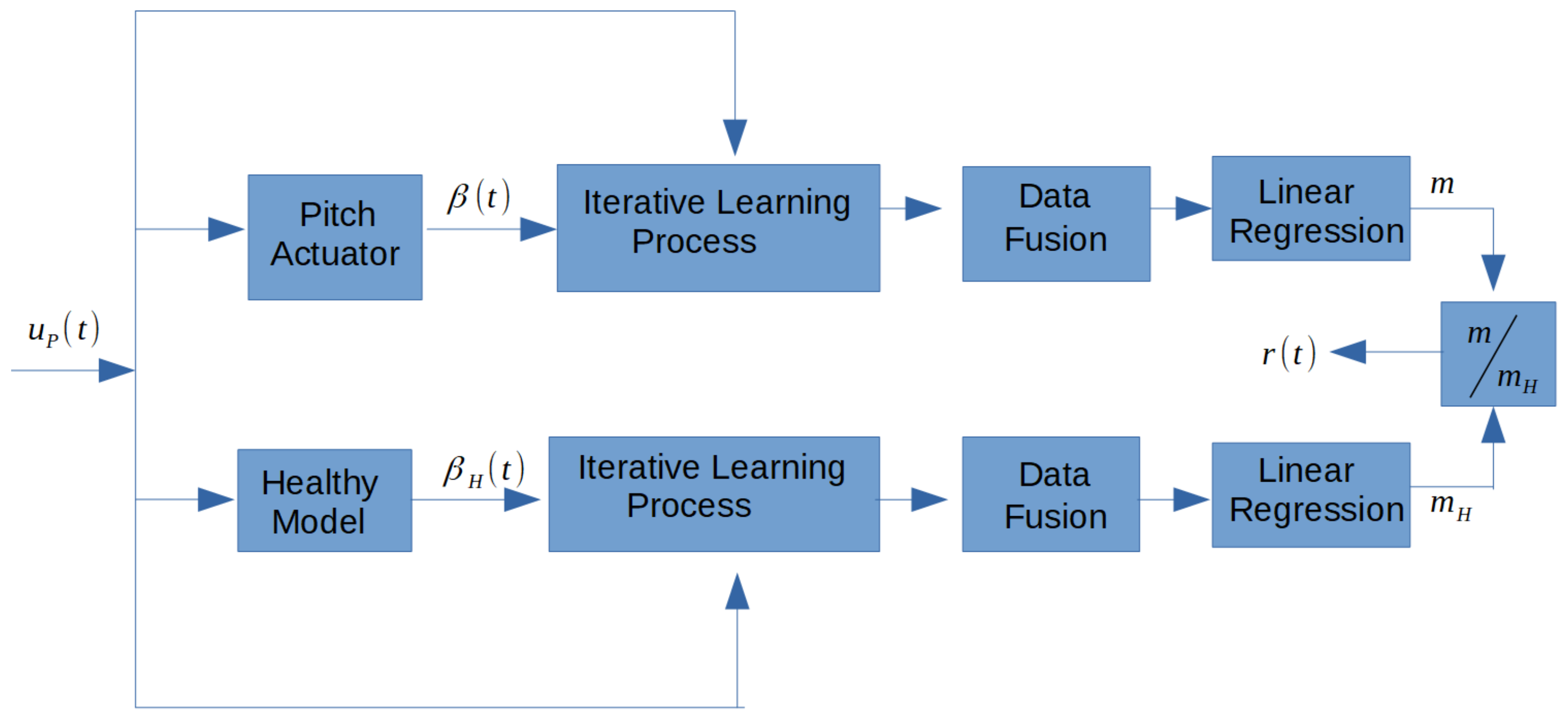
We now propose a diagnosis of pitch actuator failures based on the fusion data theory. Based on Theorem 1,
Figure 1 shows the health monitoring system proposed for the diagnosis of failures in actuator devices in wind turbines. The data employed here are presented in
Table 2 [
26]. The diagnosis is based on the following steps. Under each scenario in
Table 1, a data fusion raw
(
12) is obtained. Then, a decision parameter
m is defined in each case. First, a healthy value of
m for the nominal plant H (healthy scenario in
Table 1) is derived, referred to as
in
Figure 1. Secondly, under each faulty case, parameter
m is evaluated and compared to
to decide if a failure occurs.
First, let us define parameter
m: it corresponds to the regression of data fusion raw. That is, a linear relation is used to fit our data
in (
12) to a polynomial function of degree one, and by using minimum squares method. Therefore, the linear regression stage does this regression on the merged data and only
m, the slope of the linear regression, is implemented.
Then, to detect a pitch actuator failure, the factor is evaluated. If , a malfunction of the system has occurred, as showed in the next section.
4. Numerical Simulations
Table 2 shows the stages analyzed. Therefore, the healthy model in
Figure 1 refers to the
H scenario in
Table 1. The experimental parameter considered in pitch actuator exact model (
2), simpler model (
3) and the iterative learning algorithm (
4) are defined in
Table 1,
Table 2 and
Table 3.
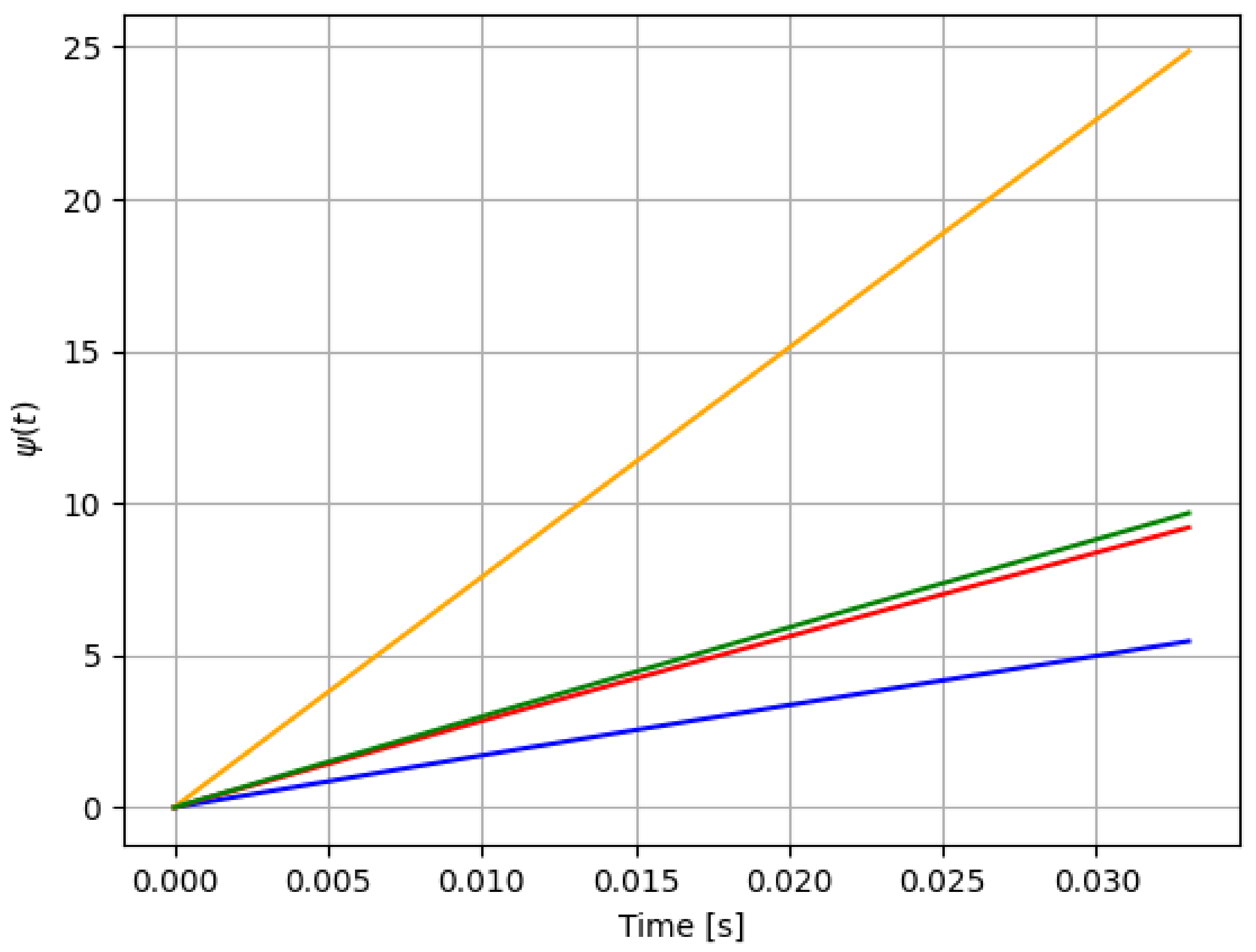
For reference, the following color labeling is used: (
H) blue, (
) red, (
) orange, and (
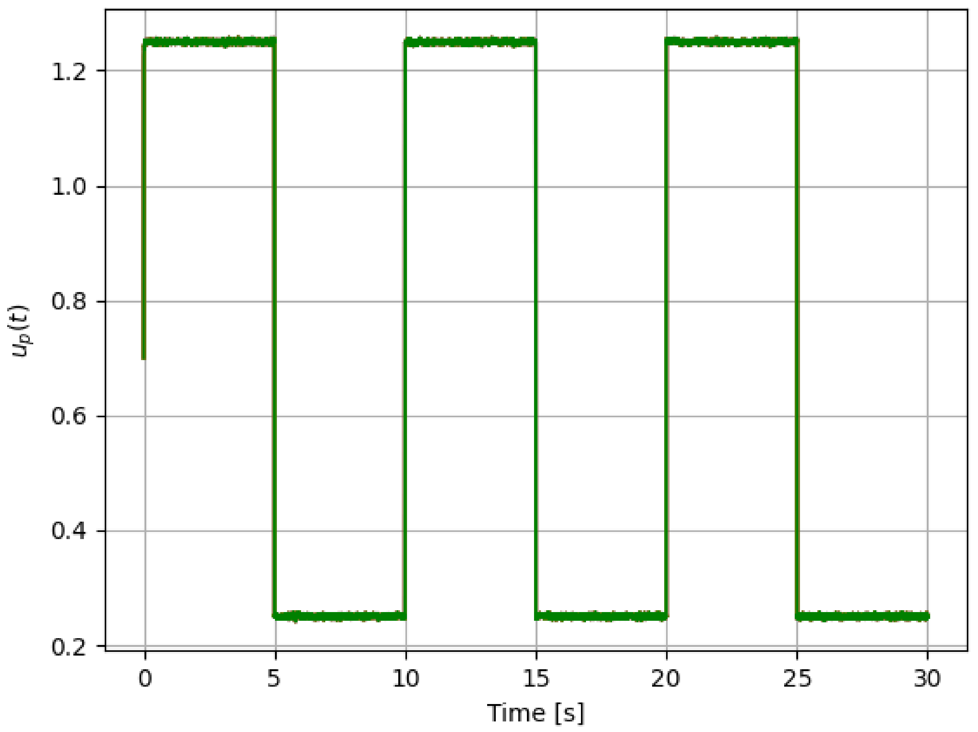
) green. By using the pitch command signal given in
Figure 2,
Figure 3 and
Figure 4 show the results of the simulation of the proposed scheme. Then, in all simulations, additive noise is attached to the pitch command signal for the robustness analysis of the proposed method.
Table 4 shows the obtained regression parameters, where in the three faulty scenarios parameter
r is greater than 1 and the detection algorithm works. Moreover,
Figure 4 pictures data fusion variable
(
4), and again the fault detection is illustrated.
Second experiment outcomes are shown in
Figure 5,
Figure 6 and
Figure 7. Once again,
Table 5 gives the reading regression parameters. From
Table 1,
Table 2,
Table 3,
Table 4 and
Table 5, a threshold to the residual signal
can be easily set to locate each failure. That is, despite the noise added to the data, our method is able to discern among the three different failure scenarios. As
Table 5 shows, the parameter
r for each case is located in a range of different values.
5. Discussion
Based on the simplest model used for the pitch actuator system (
3), and because the iterative process identifies a parameter related to the system time-constant, the best option for the iterative process is to use a stepped pitch reference command, as shown in the previous simulations. However, to see the performance of our approach, we use a sine pitch command signal as shown in
Figure 8. Numerical experiment results are shown in
Figure 9 and
Figure 10. Furthermore,
Table 6 gives the related results of the iterative process results. Even in this case, the system reacts differently to different failure cases. Although the sinusoidal signal is not commonly used as a reference in estimating the time constant of a system, our approach still allows us to detect variability of this parameter. Compared to
Table 5, the classification is not as robust, as expected when dealing with a sinusoidal input.Therefore, future work will be to design a residual signal, as for the sinusoidal pitch command, which will do the same job.


