
Intelligent Decision-Making of Scheduling for Dynamic Permutation Flowshop via Deep Reinforcement Learning


Abstract
:1. Introduction
- (1)
- To the best of our knowledge, this is the first attempt to solve the dynamic PFSP with new job arrival to minimize total tardiness cost using DRL. Our work can fill the research gap in solving dynamic PFSP by DRL.
- (2)
- An intelligent decision-making scheduling system based on DRL is designed and modeled. The system architecture of intelligent scheduling is proposed. States features, actions and reward for the scheduling agent and system are designed.
- (3)
- Our work shows the DRL-based scheduling method outperforms traditional meta-heuristics (IG and GA) in solution quantity and CPU times by a large margin for dynamic FPSP.
2. Problem Description and Mathematical Model
2.1. Problem Description
2.2. Mathematical Model
- j: index of jobs, j = 1, 2, …, n
- i: index of machines, i = 1, 2, …, m
- tij: processing time of job j on machine i, i = 1, 2, …, m, j = 1, 2, …, n
- Cij: completion time of job j on machine i, i = 1, 2, …, m, j = 1, 2, …, n
- Cj: completion time of job j, j = 1, 2, …, n
- dj: due date of job j, j = 1, 2, …, n
- CP: an indicator of completion time of all jobs
- TF: tardiness factor
- RDD: the relative range of due dates
- : unit (per second) tardiness cost of job j
- ATj: arrival time of job j
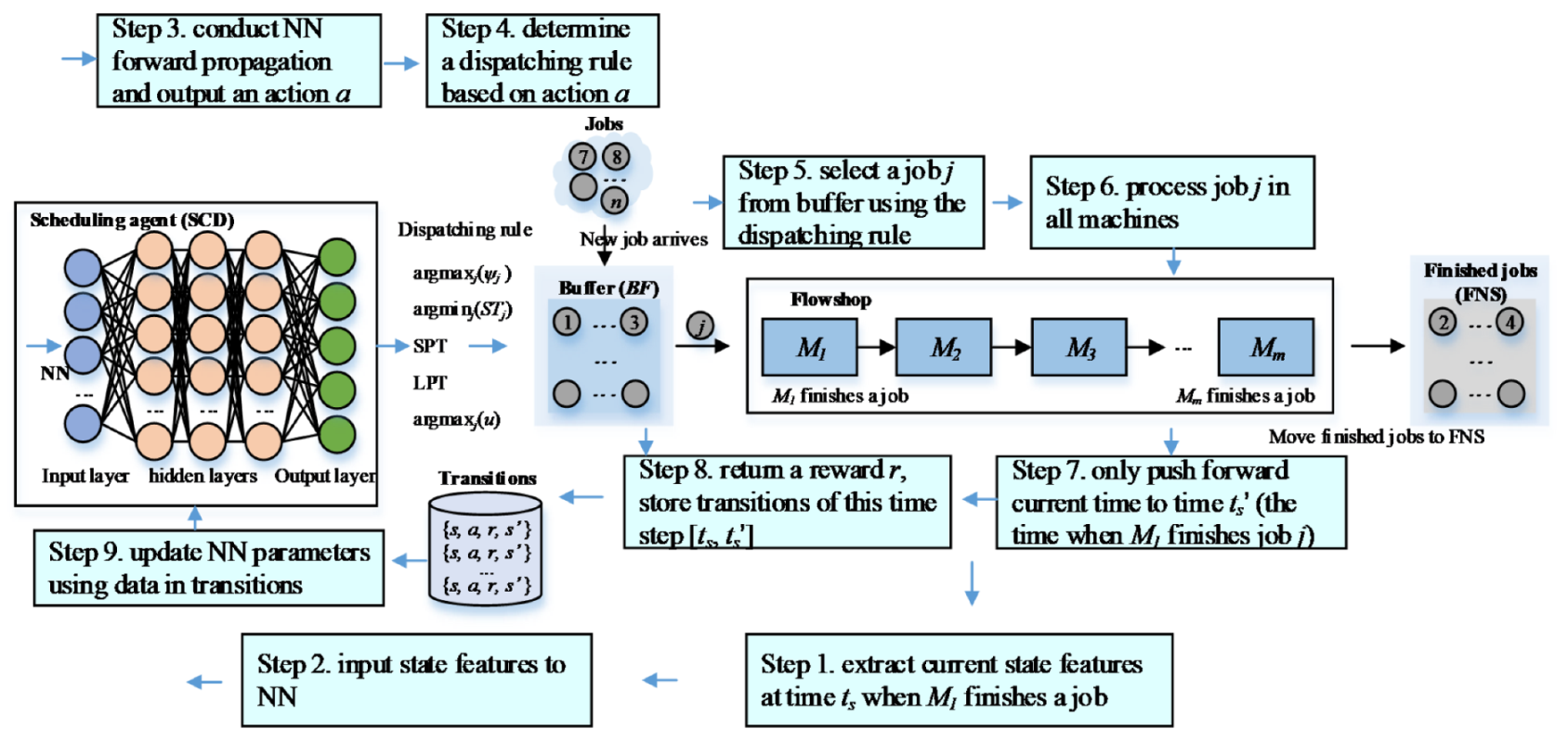
3. Modelling of the Intelligent Scheduling System
3.1. Reward
3.2. State Features
- (1)
- . Current unit tardiness cost of each job in BF.where is the unit tardiness cost generated by job j at present and is calculated as follows.
- (2)
- . Safe time of each job in BF.where STj is determined by Equation (15). STj reflects how much time will be left before the due date dj when job j is finished, if job j begins to be processed at present time tc.
- (3)
- . Total processing times in all machines for each job in BF.
- (4)
- . The estimated utilization rate of each job in BF. uj′ is the estimated utilization rate of job j and is calculated by Equation (16). Each job in BF is assumed to be processed under the present production status. The uj′ is calculated based on the waiting times WTij′ of all machines when job j is processed.where WTij′ is the waiting time of job j on machine i. WTij′ generates when job j is finished on machine i − 1, but cannot be processed immediately on machine i because machine i has not finished its current job j − 1. Note that the first machine M1 does not have a waiting time because M1 is always idle at a decision point.
- (5)
- . The number of jobs in BF at present.
3.3. Actions
4. A2C
| Algorithm 1. The A2C-based training method. |
|
5. Numerical Experiments
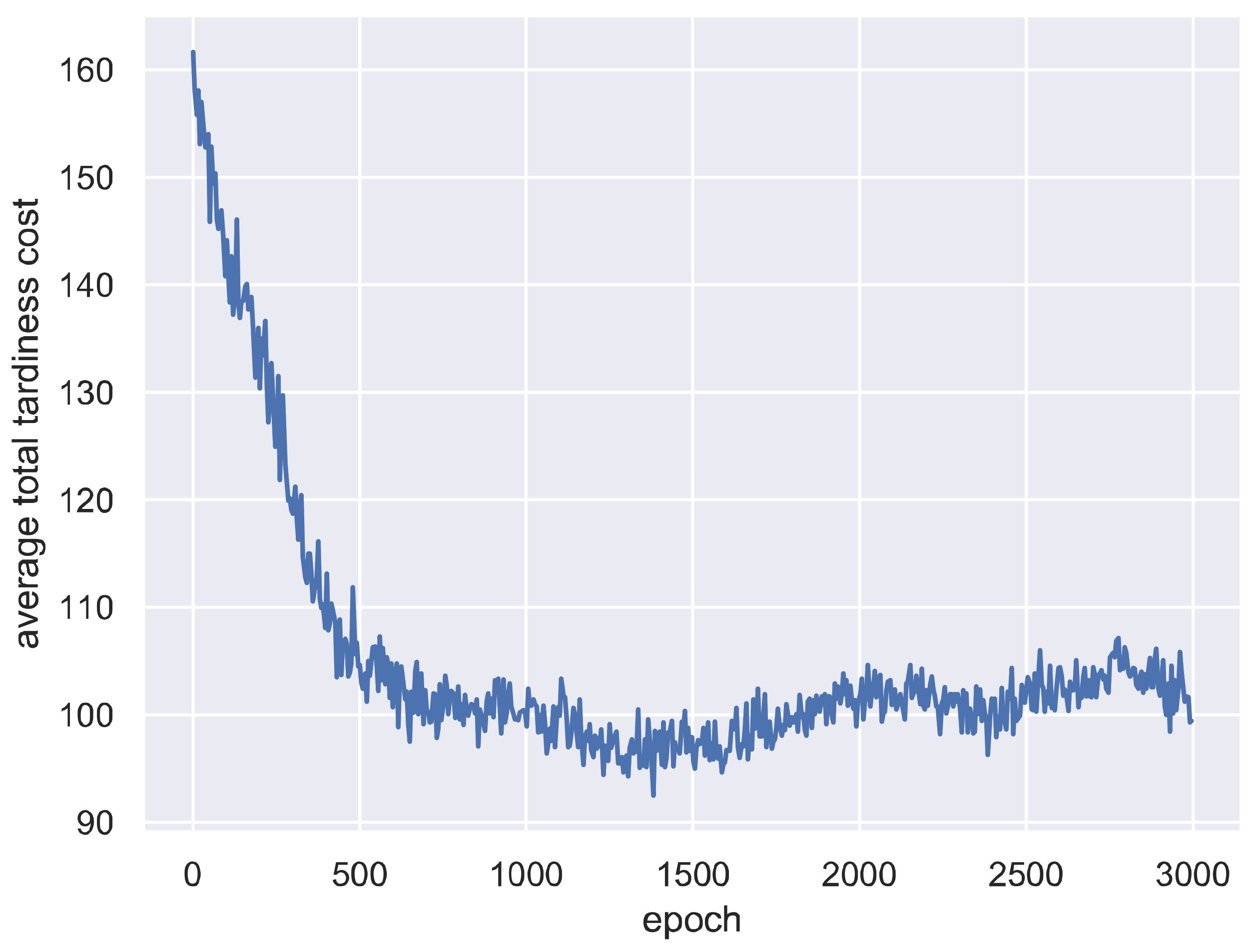
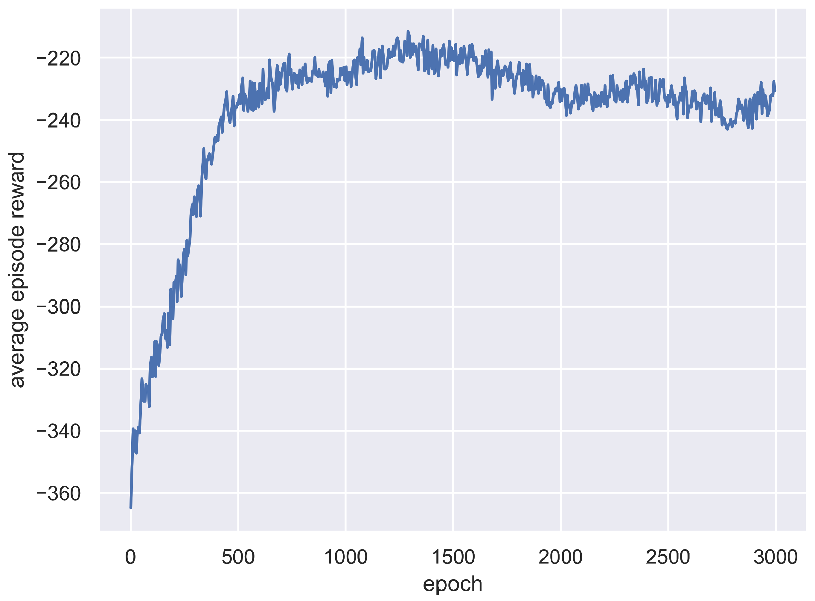
5.1. Training Process of A2C
5.2. Comparison with SDR
5.3. Comparison with DRL and Meta-Heuristics
5.3.1. Training Process of DQN and DDQN
5.3.2. IG and GA
5.3.3. Comparison with DQN, DDQN, IG, and GA
5.4. Generalization to Larger Instances
6. Conclusions
Supplementary Materials
Author Contributions
Funding
Institutional Review Board Statement
Informed Consent Statement
Data Availability Statement
Conflicts of Interest
References
- Fernandez-Viagas, V.; Ruiz, R.; Framinan, J.M. A new vision of approximate methods for the permutation flowshop to minimise makespan: State-of-the-art and computational evaluation. Eur. J. Oper. Res. 2017, 257, 707–721. [Google Scholar] [CrossRef]
- Nazhad, S.H.H.; Shojafar, M.; Shamshirband, S.; Conti, M. An efficient routing protocol for the QoS support of large-scale MANETs. Int. J. Commun. Syst. 2018, 31, e3384. [Google Scholar] [CrossRef]
- Hosseinabadi, A.A.R.; Kardgar, M.; Shojafar, M.; Shamshirband, S.; Abraham, A. GELS-GA: Hybrid Metaheuristic Algorithm for Solving Multiple Travelling Salesman Problem. In Proceedings of the 14th International Conference on Intelligent Systems Design & Applications, Okinawa, Japan, 28–30 November 2014. [Google Scholar]
- Rossi, F.L.; Nagano, M.S.; Neto, R.F.T. Evaluation of high performance constructive heuristics for the flow shop with makespan minimization. Int. J. Adv. Manuf. Technol. 2016, 87, 125–136. [Google Scholar] [CrossRef]
- Lin, J. A hybrid discrete biogeography-based optimization for the permutation flow shop scheduling problem. Int. J. Prod. Res. 2015, 54, 4805–4814. [Google Scholar] [CrossRef]
- Khatami, M.; Salehipour, A.; Hwang, F.J. Makespan minimization for the m-machine ordered flow shop scheduling problem. Comput. Oper. Res. 2019, 111, 400–414. [Google Scholar] [CrossRef]
- Santucci, V.; Baioletti, M.; Milani, A. Algebraic Differential Evolution Algorithm for the Permutation Flowshop Scheduling Problem With Total Flowtime Criterion. IEEE Trans. Evol. Comput. 2016, 20, 682–694. [Google Scholar] [CrossRef]
- Rossi, F.L.; Nagano, M.S.; Sagawa, J.K. An effective constructive heuristic for permutation flow shop scheduling problem with total flow time criterion. Int. J. Adv. Manuf. Technol. 2016, 90, 93–107. [Google Scholar] [CrossRef]
- Abedinnia, H.; Glock, C.H.; Brill, A. New simple constructive heuristic algorithms for minimizing total flow-time in the permutation flowshop scheduling problem. Comput. Oper. Res. 2016, 74, 165–174. [Google Scholar] [CrossRef]
- Deng, G.; Yang, H.; Zhang, S. An Enhanced Discrete Artificial Bee Colony Algorithm to Minimize the Total Flow Time in Permutation Flow Shop Scheduling with Limited Buffers. Math. Probl. Eng. 2016, 2016, 7373617. [Google Scholar] [CrossRef]
- Schaller, J.; Valente, J.M.S. Heuristics for scheduling jobs in a permutation flow shop to minimize total earliness and tardiness with unforced idle time allowed. Expert Syst. Appl. 2019, 119, 376–386. [Google Scholar] [CrossRef]
- Fernandez-Viagas, V.; Molina-Pariente, J.M.; Framinan, J.M. Generalised accelerations for insertion-based heuristics in permutation flowshop scheduling. Eur. J. Oper. Res. 2020, 282, 858–872. [Google Scholar] [CrossRef]
- Ta, Q.C.; Billaut, J.-C.; Bouquard, J.-L. Matheuristic algorithms for minimizing total tardiness in the m-machine flow-shop scheduling problem. J. Intell. Manuf. 2015, 29, 617–628. [Google Scholar] [CrossRef]
- Pagnozzi, F.; Stützle, T. Speeding up local search for the insert neighborhood in the weighted tardiness permutation flowshop problem. Optim. Lett. 2016, 11, 1283–1292. [Google Scholar] [CrossRef]
- Al-Behadili, M.; Ouelhadj, D.; Jones, D. Multi-objective biased randomised iterated greedy for robust permutation flow shop scheduling problem under disturbances. J. Oper. Res. Soc. 2019, 71, 1847–1859. [Google Scholar] [CrossRef]
- Valledor, P.; Gomez, A.; Priore, P.; Puente, J. Solving multi-objective rescheduling problems in dynamic permutation flow shop environments with disruptions. Int. J. Prod. Res. 2018, 56, 6363–6377. [Google Scholar] [CrossRef]
- Xu, J.; Wu, C.-C.; Yin, Y.; Lin, W.-C. An iterated local search for the multi-objective permutation flowshop scheduling problem with sequence-dependent setup times. Appl. Soft Comput. 2017, 52, 39–47. [Google Scholar] [CrossRef]
- Wang, X.; Tang, L. A machine-learning based memetic algorithm for the multi-objective permutation flowshop scheduling problem. Comput. Oper. Res. 2017, 79, 60–77. [Google Scholar] [CrossRef]
- Li, X.; Ma, S. Multi-Objective Memetic Search Algorithm for Multi-Objective Permutation Flow Shop Scheduling Problem. IEEE Access 2016, 4, 2154–2165. [Google Scholar] [CrossRef]
- González-Neira, E.M.; Urrego-Torres, A.M.; Cruz-Riveros, A.M.; Henao-García, C.; Montoya-Torres, J.R.; Molina-Sánchez, L.P.; Jiménez, J.-F. Robust solutions in multi-objective stochastic permutation flow shop problem. Comput. Ind. Eng. 2019, 137, 106026. [Google Scholar] [CrossRef]
- Dubois-Lacoste, J.; Pagnozzi, F.; Stützle, T. An iterated greedy algorithm with optimization of partial solutions for the makespan permutation flowshop problem. Comput. Oper. Res. 2017, 81, 160–166. [Google Scholar] [CrossRef]
- Karabulut, K. A hybrid iterated greedy algorithm for total tardiness minimization in permutation flowshops. Comput. Ind. Eng. 2016, 98, 300–307. [Google Scholar] [CrossRef]
- Fernandez-Viagas, V.; Valente, J.M.S.; Framinan, J.M. Iterated-greedy-based algorithms with beam search initialization for the permutation flowshop to minimise total tardiness. Expert Syst. Appl. 2018, 94, 58–69. [Google Scholar] [CrossRef] [Green Version]
- Fernandez-Viagas, V.; Framinan, J.M. A best-of-breed iterated greedy for the permutation flowshop scheduling problem with makespan objective. Comput. Oper. Res. 2019, 112, 104767. [Google Scholar] [CrossRef]
- Rahman, H.F.; Janardhanan, M.N.; Nielsen, I.E. Real-Time Order Acceptance and Scheduling Problems in a Flow Shop Environment Using Hybrid GA-PSO Algorithm. IEEE Access 2019, 7, 112742–112755. [Google Scholar] [CrossRef]
- Tasgetiren, M.F.; Liang, Y.-C.; Sevkli, M.; Gencyilmaz, G. A particle swarm optimization algorithm for makespan and total flowtime minimization in the permutation flowshop sequencing problem. Eur. J. Oper. Res. 2007, 177, 1930–1947. [Google Scholar] [CrossRef]
- Marinakis, Y.; Marinaki, M. Particle swarm optimization with expanding neighborhood topology for the permutation flowshop scheduling problem. Soft Comput. 2013, 17, 1159–1173. [Google Scholar] [CrossRef]
- Wang, Z.; Zhang, J.; Yang, S. An improved particle swarm optimization algorithm for dynamic job shop scheduling problems with random job arrivals. Swarm Evol. Comput. 2019, 51, 100594. [Google Scholar] [CrossRef]
- Chen, J.; Wang, M.; Kong, X.T.R.; Huang, G.Q.; Dai, Q.; Shi, G. Manufacturing synchronization in a hybrid flowshop with dynamic order arrivals. J. Intell. Manuf. 2017, 30, 2659–2668. [Google Scholar] [CrossRef]
- Baykasoğlu, A.; Karaslan, F.S. Solving comprehensive dynamic job shop scheduling problem by using a GRASP-based approach. Int. J. Prod. Res. 2017, 55, 3308–3325. [Google Scholar] [CrossRef]
- Moghaddam, S.K.; Saitou, K. On optimal dynamic pegging in rescheduling for new order arrival. Comput. Ind. Eng. 2019, 136, 46–56. [Google Scholar] [CrossRef]
- Framinan, J.M.; Fernandez-Viagas, V.; Perez-Gonzalez, P. Using real-time information to reschedule jobs in a flowshop with variable processing times. Comput. Ind. Eng. 2019, 129, 113–125. [Google Scholar] [CrossRef]
- Baker, K.R.; Altheimer, D. Heuristic solution methods for the stochastic flow shop problem. Eur. J. Oper. Res. 2012, 216, 172–177. [Google Scholar] [CrossRef]
- Villarinho, P.A.; Panadero, J.; Pessoa, L.S.; Juan, A.A.; Oliveira, F.L.C. A simheuristic algorithm for the stochastic permutation flow-shop problem with delivery dates and cumulative payoffs. Int. Trans. Oper. Res. 2020, 28, 716–737. [Google Scholar] [CrossRef]
- Liu, F.; Wang, S.; Hong, Y.; Yue, X. On the Robust and Stable Flowshop Scheduling Under Stochastic and Dynamic Disruptions. IEEE Trans. Eng. Manag. 2017, 64, 539–553. [Google Scholar] [CrossRef]
- Valledor, P.; Gomez, A.; Priore, P.; Puente, J. Modelling and Solving Rescheduling Problems in Dynamic Permutation Flow Shop Environments. Complexity 2020, 2020, 2862186. [Google Scholar] [CrossRef]
- Rahman, H.F.; Sarker, R.; Essam, D. Multiple-order permutation flow shop scheduling under process interruptions. Int. J. Adv. Manuf. Technol. 2018, 97, 2781–2808. [Google Scholar] [CrossRef]
- Rahman, H.F.; Sarker, R.; Essam, D. A real-time order acceptance and scheduling approach for permutation flow shop problems. Eur. J. Oper. Res. 2015, 247, 488–503. [Google Scholar] [CrossRef]
- Shiue, Y.R.; Lee, K.C.; Su, C.T. Real-time scheduling for a smart factory using a reinforcement learning approach. Comput. Ind. Eng. 2018, 125, 604–614. [Google Scholar] [CrossRef]
- Hosseinabadi, A.A.R.; Siar, H.; Shamshirband, S.; Shojafar, M.; Nasir, M.H.N.M. Using the gravitational emulation local search algorithm to solve the multi-objective flexible dynamic job shop scheduling problem in Small and Medium Enterprises. Ann. Oper. Res. 2014, 229, 451–474. [Google Scholar] [CrossRef]
- Liu, W.; Jin, Y.; Price, M. New scheduling algorithms and digital tool for dynamic permutation flowshop with newly arrived order. Int. J. Prod. Res. 2017, 55, 3234–3248. [Google Scholar] [CrossRef] [Green Version]
- Li, G.; Li, N.; Sambandam, N.; Sethi, S.P.; Zhang, F. Flow shop scheduling with jobs arriving at different times. Int. J. Prod. Econ. 2018, 206, 250–260. [Google Scholar] [CrossRef]
- Liu, W.; Jin, Y.; Price, M. New meta-heuristic for dynamic scheduling in permutation flowshop with new order arrival. Int. J. Adv. Manuf. Technol. 2018, 98, 1817–1830. [Google Scholar] [CrossRef] [Green Version]
- Luo, S. Dynamic scheduling for flexible job shop with new job insertions by deep reinforcement learning. Appl. Soft Comput. 2020, 91, 106208. [Google Scholar] [CrossRef]
- Zhang, Z.C.; Wang, W.P.; Zhong, S.Y.; Hu, K.S. Flow Shop Scheduling with Reinforcement Learning. Asia Pac. J. Oper. Res. 2013, 30, 1350014. [Google Scholar] [CrossRef]
- Lin, C.C.; Deng, D.J.; Chih, Y.L.; Chiu, H.T. Smart Manufacturing Scheduling With Edge Computing Using Multiclass Deep Q Network. IEEE Trans. Ind. Inform. 2019, 15, 4276–4284. [Google Scholar] [CrossRef]
- Liu, C.L.; Chang, C.C.; Tseng, C.J. Actor-Critic Deep Reinforcement Learning for Solving Job Shop Scheduling Problems. IEEE Access 2020, 8, 71752–71762. [Google Scholar] [CrossRef]
- Zhang, C.; Song, W.; Cao, Z.; Zhang, J.; Tan, P.S.; Xu, C. Learning to Dispatch for Job Shop Scheduling via Deep Reinforcement Learning. arXiv 2020, arXiv:2010.12367. [Google Scholar]
- Han, B.-A.; Yang, J.-J. Research on Adaptive Job Shop Scheduling Problems Based on Dueling Double DQN. IEEE Access 2020, 8, 186474–186495. [Google Scholar] [CrossRef]
- Wang, H.X.; Sarker, B.R.; Li, J.; Li, J. Adaptive scheduling for assembly job shop with uncertain assembly times based on dual Q-learning. Int. J. Prod. Res. 2020, 1–17. [Google Scholar] [CrossRef]
- Shiue, Y.-R.; Lee, K.-C.; Su, C.-T. A Reinforcement Learning Approach to Dynamic Scheduling in a Product-Mix Flexibility Environment. IEEE Access 2020, 8, 106542–106553. [Google Scholar] [CrossRef]
- Zhang, Z.C.; Zheng, L.; Li, N.; Wang, W.P.; Zhong, S.Y.; Hu, K.S. Minimizing mean weighted tardiness in unrelated parallel machine scheduling with reinforcement learning. Comput. Oper. Res. 2012, 39, 1315–1324. [Google Scholar] [CrossRef]
- Jun, S.; Lee, S. Learning dispatching rules for single machine scheduling with dynamic arrivals based on decision trees and feature construction. Int. J. Prod. Res. 2020, 20, 1–19. [Google Scholar] [CrossRef]
- Wu, C.H.; Zhou, F.Y.; Tsai, C.K.; Yu, C.J.; Dauzere-Peres, S. A deep learning approach for the dynamic dispatching of unreliable machines in re-entrant production systems. Int. J. Prod. Res. 2020, 58, 2822–2840. [Google Scholar] [CrossRef]
- Li, Y.Y.; Carabelli, S.; Fadda, E.; Manerba, D.; Tadei, R.; Terzo, O. Machine learning and optimization for production rescheduling in Industry 4.0. Int. J. Adv. Manuf. Technol. 2020, 110, 2445–2463. [Google Scholar] [CrossRef]
- Chen, R.; Yang, B.; Li, S.; Wang, S. A self-learning genetic algorithm based on reinforcement learning for flexible job-shop scheduling problem. Comput. Ind. Eng. 2020, 149, 106778. [Google Scholar] [CrossRef]
- Wang, K.; Luo, H.; Liu, F.; Yue, X. Permutation Flow Shop Scheduling With Batch Delivery to Multiple Customers in Supply Chains. IEEE Trans. Syst. ManCybern. Syst. 2018, 48, 1826–1837. [Google Scholar] [CrossRef]
- Yang, S.; Xu, Z. The distributed assembly permutation flowshop scheduling problem with flexible assembly and batch delivery. Int. J. Prod. Res. 2020, 1–19. [Google Scholar] [CrossRef]
- Wang, K.; Ma, W.Q.; Luo, H.; Qin, H. Coordinated scheduling of production and transportation in a two-stage assembly flowshop. Int. J. Prod. Res. 2016, 54, 6891–6911. [Google Scholar] [CrossRef]
- Kazemi, H.; Mazdeh, M.M.; Rostami, M. The two stage assembly flow-shop scheduling problem with batching and delivery. Eng. Appl. Artif. Intell. 2017, 63, 98–107. [Google Scholar] [CrossRef]
- Basir, S.A.; Mazdeh, M.M.; Namakshenas, M. Bi-level genetic algorithms for a two-stage assembly flow-shop scheduling problem with batch delivery system. Comput. Ind. Eng. 2018, 126, 217–231. [Google Scholar] [CrossRef]
- Mnih, V.; Badia, A.P.; Mirza, M.; Graves, A.; Lillicrap, T.; Harley, T.; Silver, D.; Kavukcuoglu, K. Asynchronous Methods for Deep Reinforcement Learning. In Proceedings of the 33rd International conference on Machine Learning, New York, NY, USA, 19–24 June 2016; pp. 1928–1937. [Google Scholar]
- Mnih, V.; Kavukcuoglu, K.; Silver, D.; Graves, A.; Antonoglou, I.; Wierstra, D.; Riedmiller, M. Playing atari with deep reinforcement learning. arXiv 2013, arXiv:1312.5602. [Google Scholar]
- Van Hasselt, H.; Guez, A.; Silver, D. Deep reinforcement learning with double q-learning. arXiv 2015, arXiv:1509.06461. [Google Scholar]
- Pan, Q.-K.; Gao, L.; Xin-Yu, L.; Jose, F.M. Effective constructive heuristics and meta-heuristics for the distributed assembly permutation flowshop scheduling problem. Appl. Soft Comput. 2019, 81, 105492. [Google Scholar] [CrossRef]


| Parameter | Value |
|---|---|
| Number of jobs (n) | {20, 50, 80, 100, 120, 150, 200} |
| Number of machines (m) | {5, 10, 15, 20} |
| Number of initial jobs for every instance | 3 |
| Interval time of job arriving | E(1/30) |
| Processing time on a machine (tij) | U[1, 100] |
| Unit tardiness cost of a job (αj) | U[0, 5] |
| Parameter | Value |
|---|---|
| Number of hidden layers | 3 |
| Number of neurons in each hidden layer | 100 |
| Number training epochs (EP) | 3000 |
| Discount factor (γ) | 0.98 |
| Update step iteration (T) | 5 |
| Learning rate of actor and critic | , |
| Range of entropy coefficient () | 0.005~0.0005 |
| DRL | Meta-Heuristics | |||||||
|---|---|---|---|---|---|---|---|---|
| 50 Iterations | 300 Iterations | |||||||
| DQN | DDQN | A2C | IG | GA | IG | GA | ||
| n | 20 | 13.88 | 21.52 | 16.06 | 19.34 | 17.68 | 19.16 | 19.67 |
| 50 | 50.09 | 65.61 | 48.98 | 75.43 | 75.83 | 73.38 | 77.13 | |
| 80 | 94.76 | 83.05 | 60.79 | 114.45 | 112.9 | 115.62 | 112.69 | |
| 100 | 101.31 | 143.59 | 108.57 | 161.13 | 159.64 | 161.99 | 165.87 | |
| 120 | 152.35 | 208.83 | 144.45 | 205.15 | 204.78 | 201.4 | 207.9 | |
| 150 | 175.06 | 190.7 | 163.28 | 222.84 | 213.67 | 220.35 | 211.7 | |
| 200 | 150.53 | 172.42 | 197.99 | 255.62 | 256.19 | 282.16 | 246.4 | |
| m | 5 | 43.76 | 63.19 | 46.76 | 50.94 | 50.04 | 50.41 | 49.21 |
| 10 | 73.73 | 78.09 | 74.81 | 101.02 | 100.75 | 106.84 | 101.21 | |
| 15 | 113.44 | 191.28 | 106.21 | 195.85 | 193.4 | 192.31 | 195.48 | |
| 20 | 265.5 | 249.54 | 232.93 | 323.72 | 316.15 | 317.65 | 321.87 | |
| Ave | 105.55 | 128.52 | 99.79 | 145.39 | 145.28 | 143.25 | 144.58 | |
| DRL | Meta-Heuristics | |||||||
|---|---|---|---|---|---|---|---|---|
| 50 Iterations | 300 Iterations | |||||||
| DQN | DDQN | A2C | IG | GA | IG | GA | ||
| n | 20 | 0.03 | 0.03 | 0.02 | 12.8 | 56.62 | 4.35 | 32.45 |
| 50 | 0.09 | 0.09 | 0.07 | 63.94 | 230.29 | 10.31 | 54.08 | |
| 80 | 0.19 | 0.18 | 0.15 | 63.2 | 278.19 | 6.39 | 37.85 | |
| 100 | 0.27 | 0.26 | 0.21 | 337.07 | 1301.06 | 15.84 | 94.28 | |
| 120 | 0.33 | 0.34 | 0.27 | 751.39 | 2791.67 | 25.53 | 121.65 | |
| 150 | 0.49 | 0.49 | 0.38 | 1020.36 | 3909.1 | 21.25 | 165.13 | |
| 200 | 0.68 | 0.69 | 0.49 | 3441.1 | 13023.42 | 34.01 | 200.35 | |
| m | 5 | 0.17 | 0.16 | 0.14 | 246.99 | 914.52 | 10.82 | 70.21 |
| 10 | 0.24 | 0.23 | 0.18 | 594.53 | 2258.63 | 13.82 | 81.65 | |
| 15 | 0.31 | 0.31 | 0.24 | 514.63 | 1665.1 | 17.72 | 89.91 | |
| 20 | 0.41 | 0.42 | 0.33 | 900.46 | 3891.24 | 24.32 | 156.79 | |
| Ave | 0.26 | 0.26 | 0.21 | 526.99 | 15.59 | 2001 | 92.45 | |
Publisher’s Note: MDPI stays neutral with regard to jurisdictional claims in published maps and institutional affiliations. |
© 2021 by the authors. Licensee MDPI, Basel, Switzerland. This article is an open access article distributed under the terms and conditions of the Creative Commons Attribution (CC BY) license (http://creativecommons.org/licenses/by/4.0/).
Share and Cite
Yang, S.; Xu, Z.; Wang, J. Intelligent Decision-Making of Scheduling for Dynamic Permutation Flowshop via Deep Reinforcement Learning. Sensors 2021, 21, 1019. https://doi.org/10.3390/s21031019
Yang S, Xu Z, Wang J. Intelligent Decision-Making of Scheduling for Dynamic Permutation Flowshop via Deep Reinforcement Learning. Sensors. 2021; 21(3):1019. https://doi.org/10.3390/s21031019
Chicago/Turabian StyleYang, Shengluo, Zhigang Xu, and Junyi Wang. 2021. "Intelligent Decision-Making of Scheduling for Dynamic Permutation Flowshop via Deep Reinforcement Learning" Sensors 21, no. 3: 1019. https://doi.org/10.3390/s21031019