A Distributed Multi-Hop Intra-Clustering Approach Based on Neighbors Two-Hop Connectivity for IoT Networks


Abstract
:1. Introduction
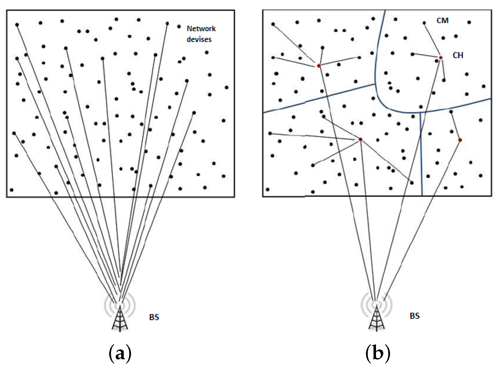
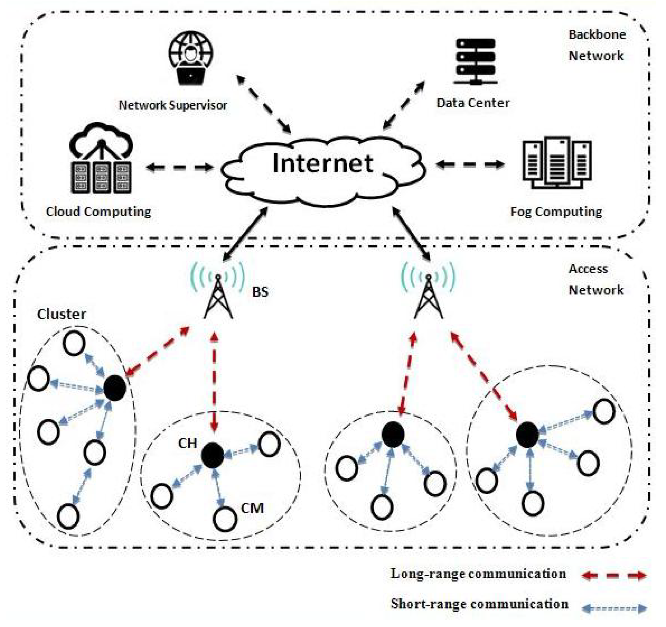
1.1. Network Architecture
1.2. Motivation
- A new connectivity metric is introduced to elect the set of appropriate CHs. The novelty of this metric is taking into account the two-hop connectivity of the current node and its surrounding neighborhood (instead of using the traditional direct neighbors connectivity), in order to strengthen the clusters stability.
- The design of the algorithm is inspired from the distributed self-stabilizing systems. We prove that the algorithm converges within rounds, which represents the upper bound of the time complexity, n is the number of network nodes and k is the depth threshold of the clusters. This perspective allows network devices to efficiently tolerate potential failures that can occur locally in the dynamic topology.
- The proposed approach generates clusters with an energy efficient topology by reducing the distance between nodes and their respective CH. The adopted approach is peculiar in that it constructs the intra-cluster links in a distributed manner rather than using a centralized algorithm executed by the CH.
2. Literature Review
3. Network Model and Algorithm Objective
4. Proposed Approach
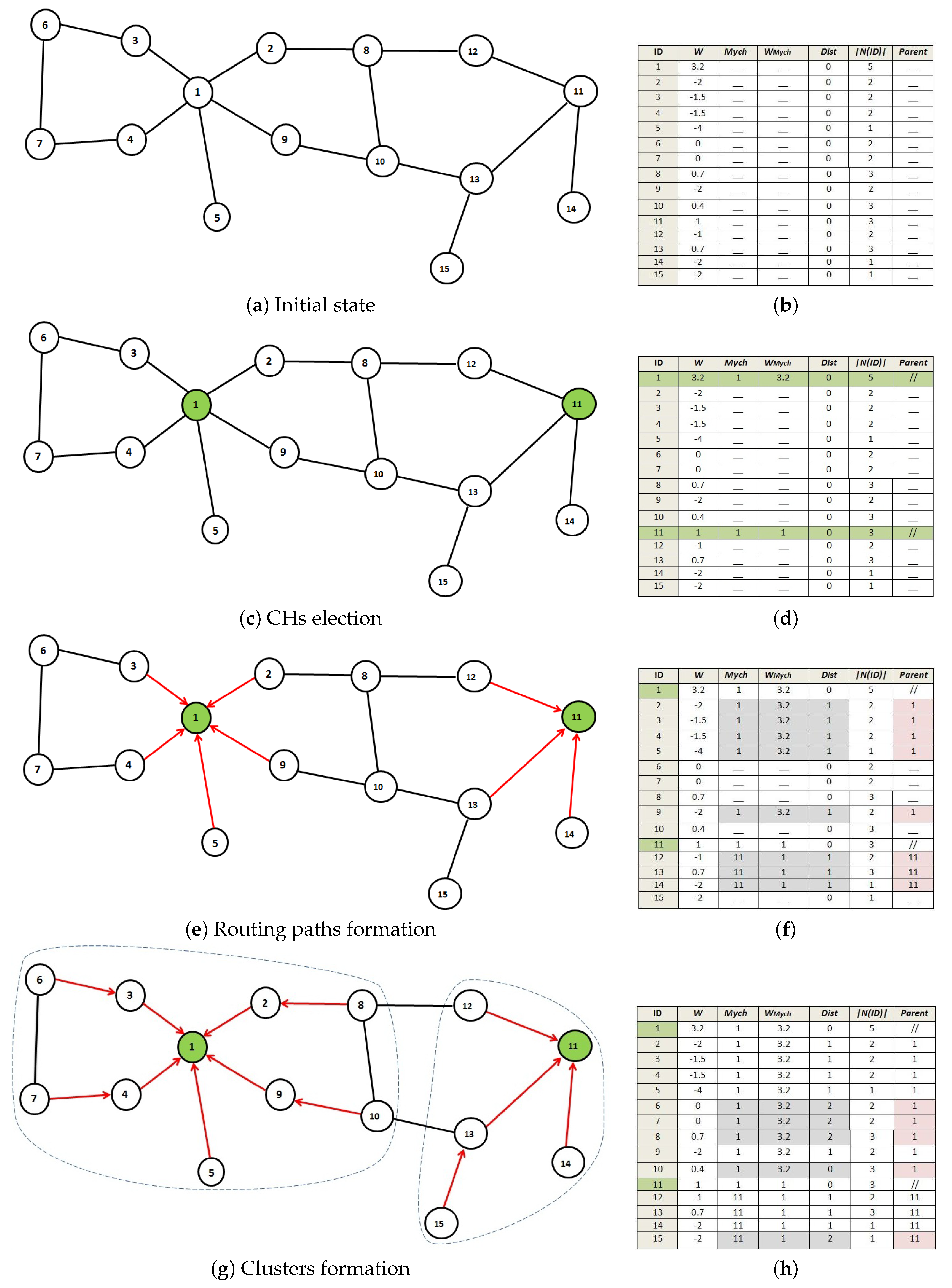
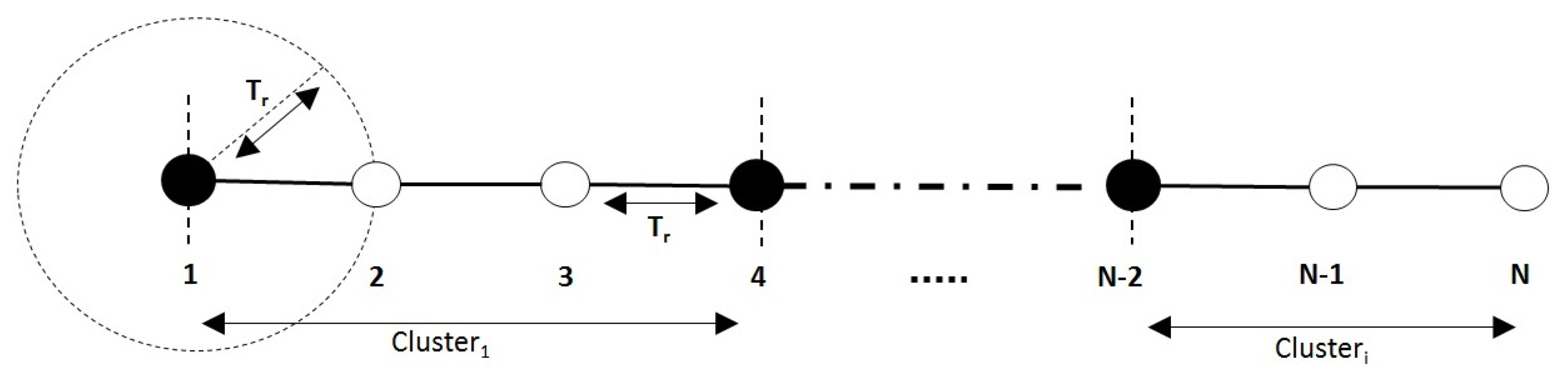
- Two-hop connectivity ratio (TCR): this parameter represents the connectivity ratio of a node relative to its neighborhood. The value of a given node i is calculated using Equation (2). Each node computes the average connectivity within its two hop neighborhood () using , then compares the obtained value with the local degree to define the . A negative value () reflects the low connectivity proportion of the node i relatively to its surrounding environment. Higher value means that node i is surrounded by a large number of neighbors and these neighbors are well connected with many other nodes, thus i is a suitable CH candidate to maintain network connectivity. Therefore, it covers the largest number of nodes within the maximum hop constraint k and generates more fault tolerant and stable cluster topology. Indeed, in case of potential CH failure, the neighborhood of this node is well connected and the replacement of the current CH does not affect the cluster performance.
- Residual energy (): the remaining energy of network nodes is introduced in the CH election process. The ratio of remaining energy of a node i is computed as:where is the initial energy of the current device and is its remaining energy.
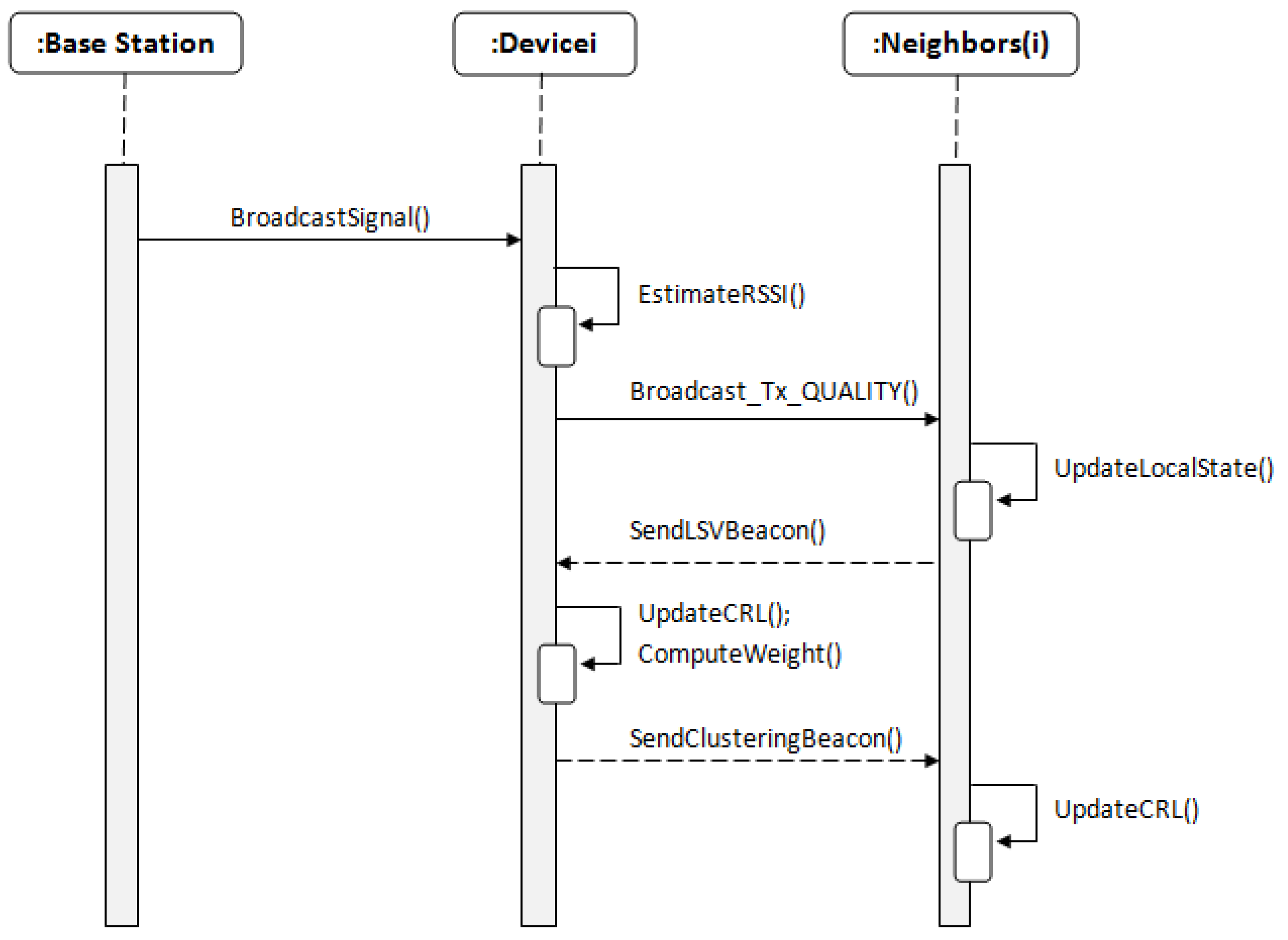
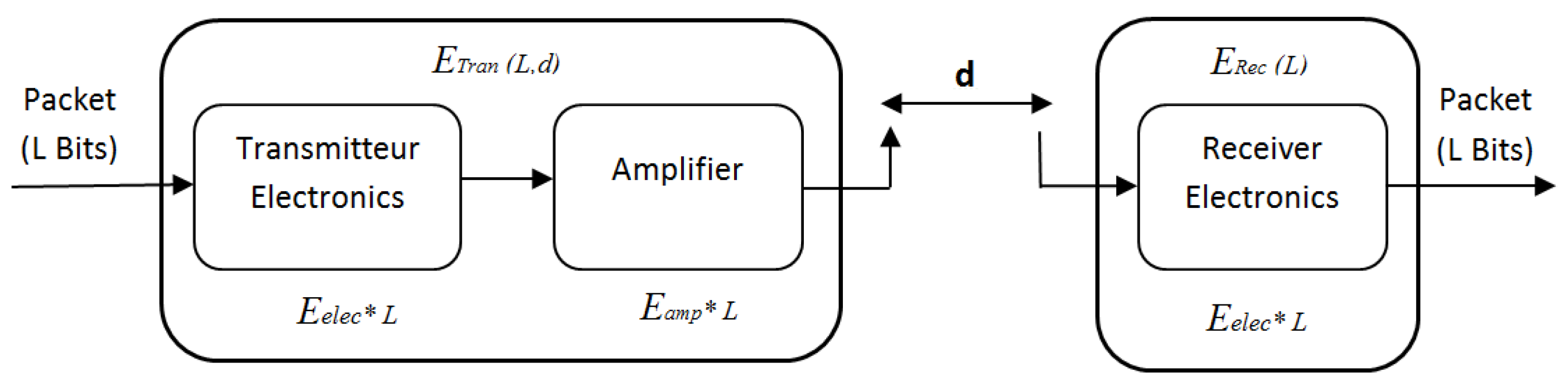
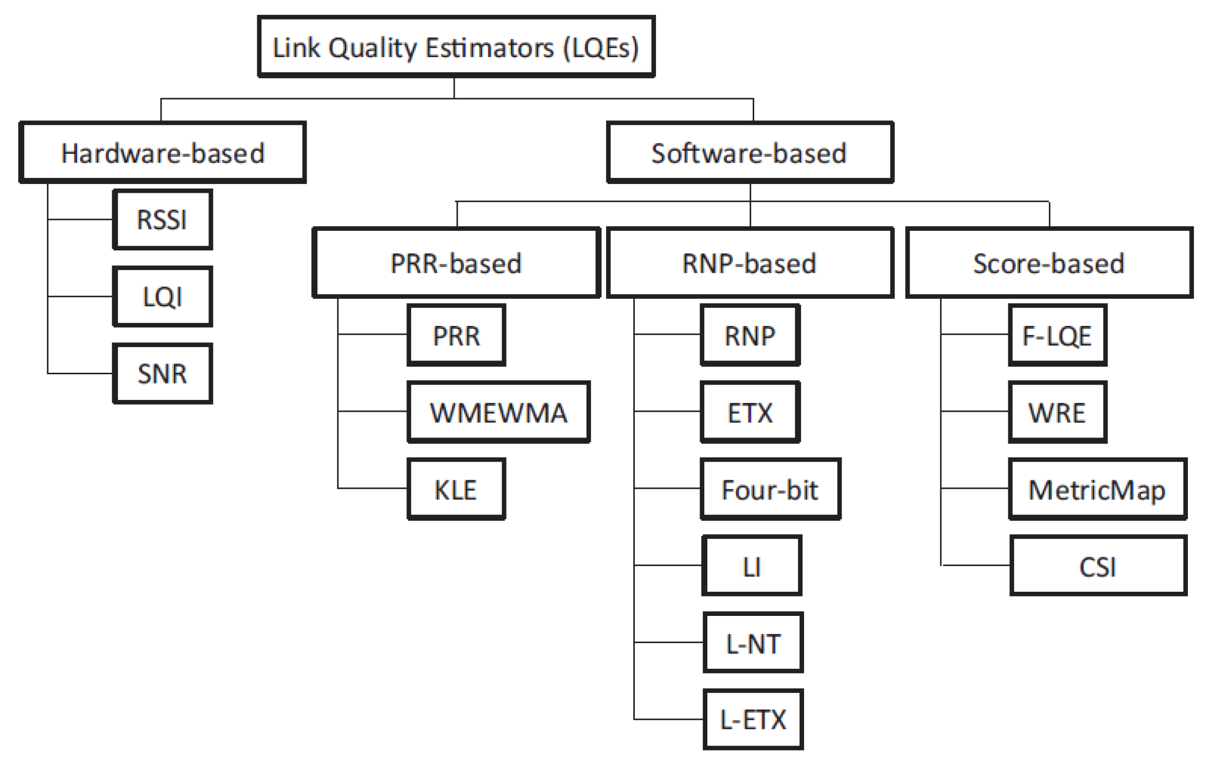
- Communication link quality (RSSI): DC2HC uses Radio Signal Strength Indicator (RSSI) as a metric to measure the quality of communications. The RSSI value (the received transmission power ) can be represented by the Log Distance Path Loss Model [53] as follows:represents the power of the transmitter’s radio signal in dBm. The distance d between the sender and the receiver is measured in meter. is the path loss exponent that depends on the environmental conditions ( in the free space propagation model). is a Gaussian random variable used in case of shadowing effect. Otherwise, it equals zero.
4.1. Initialization Phase
| Algorithm 1 Initialization phase. |
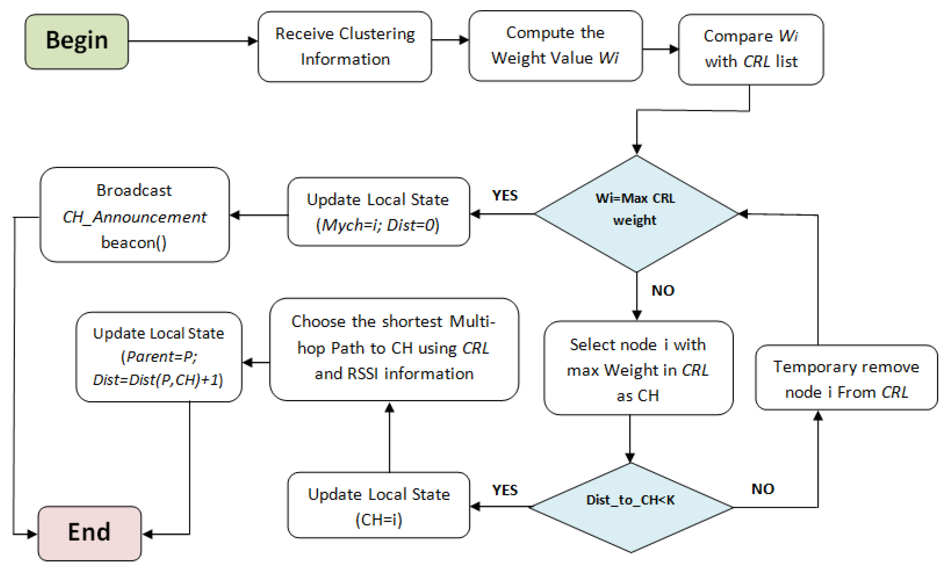
4.2. Cluster Head Election Phase
| Algorithm 2 Cluster Head election phase. |
|
4.3. Maintenance
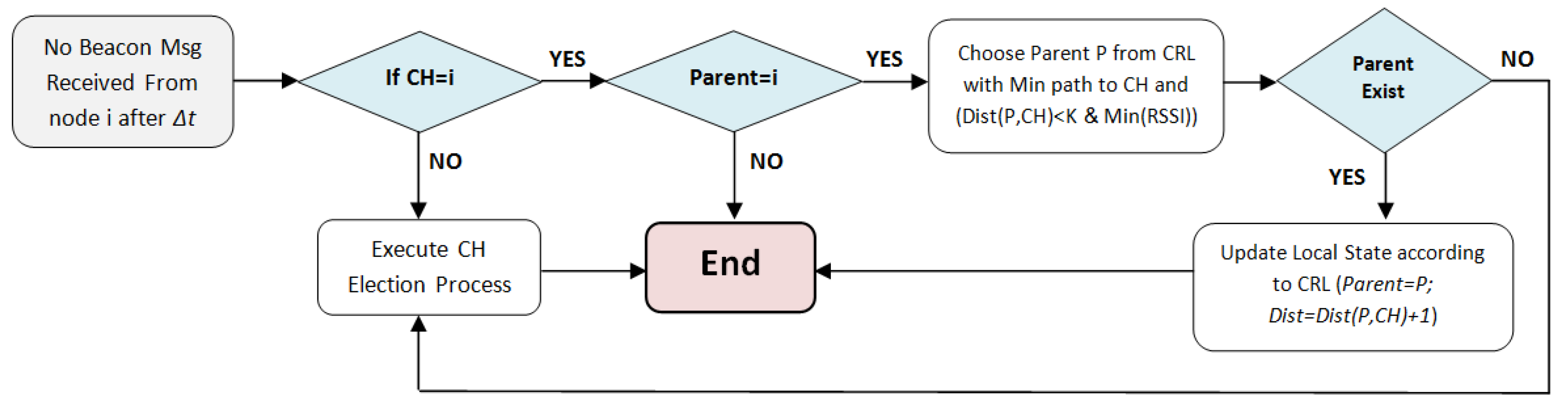
4.3.1. Cluster Leaving
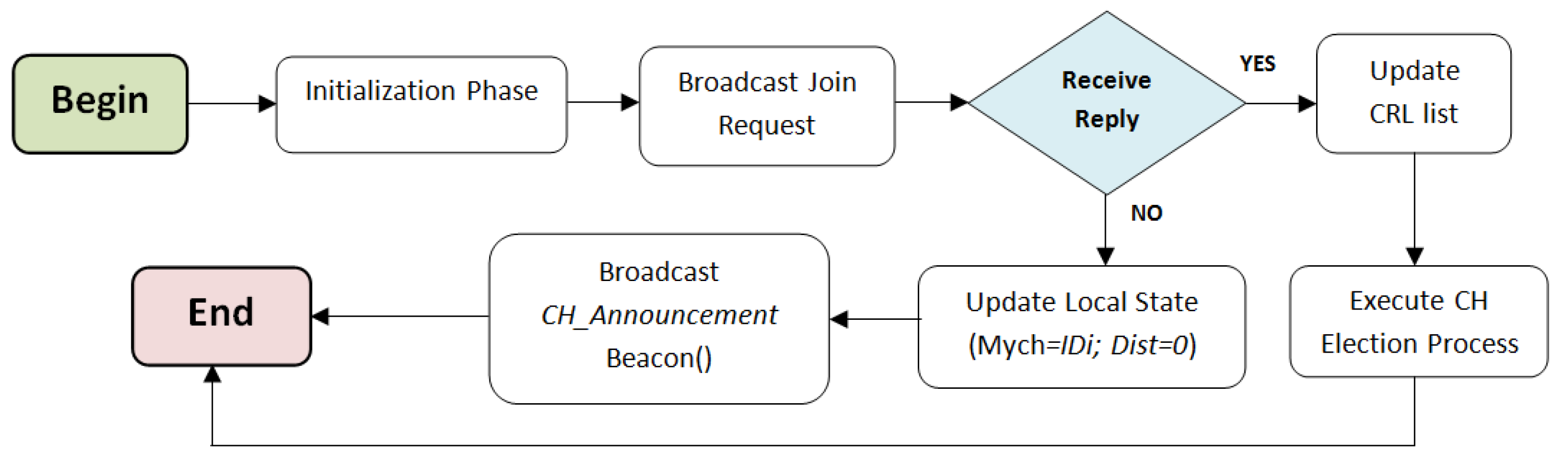
4.3.2. Cluster Joining
5. Energy Model and Transmission Reliability
6. Convergence
7. Complexity
7.1. Theoretical Analysis
- (a)
- After 2 rounds and in all following rounds, i is a cluster head ( and ).
- (b)
- After rounds and in all following rounds, the neighbors of node i at distance form a cluster, where .
7.2. Clustering Property
7.2.1. Safety Property
7.2.2. Liveness Property
8. Simulation
8.1. Experimental Settings
8.2. Experimental Results
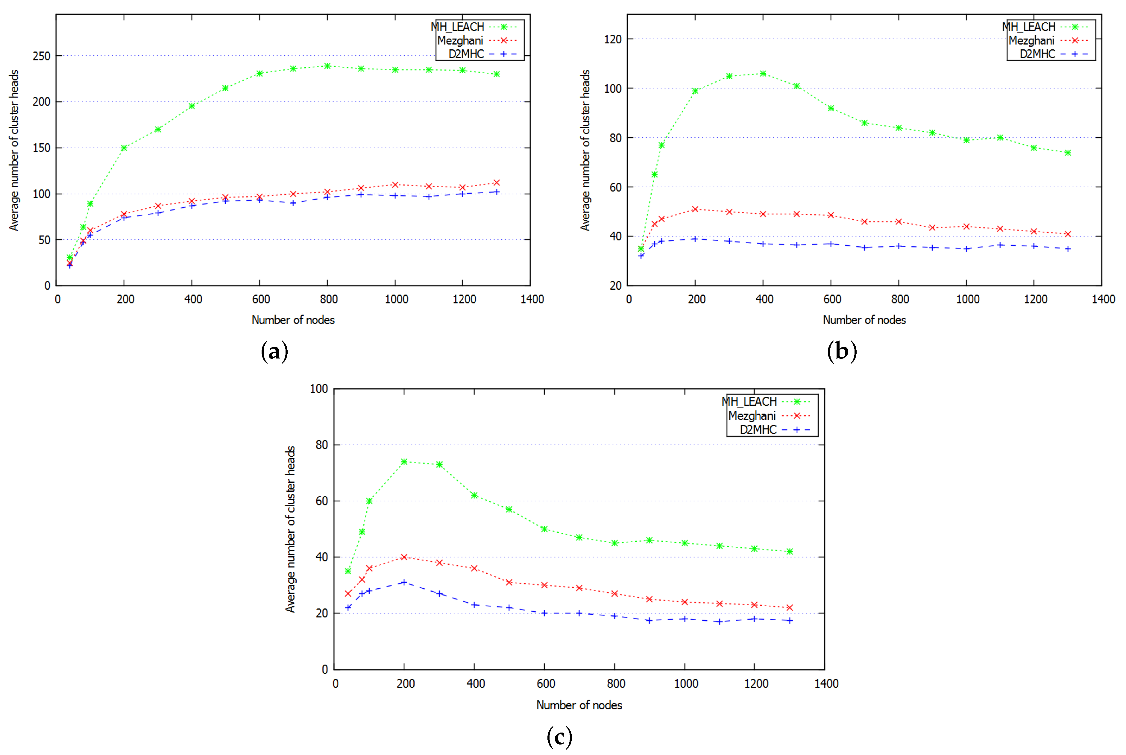
8.2.1. Cluster Head Cardinality
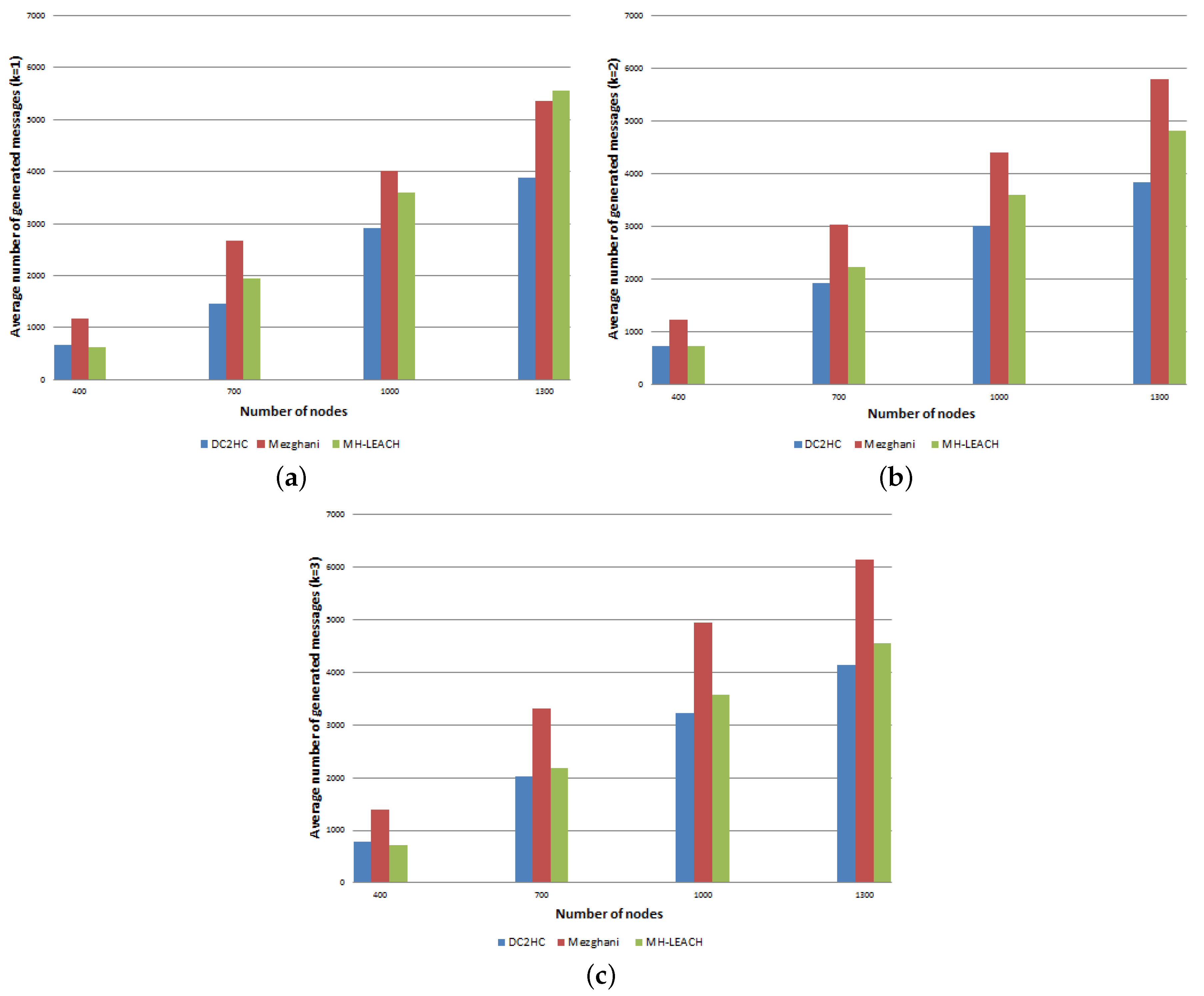
8.2.2. Average Exchanged Messages and Consumed Energy
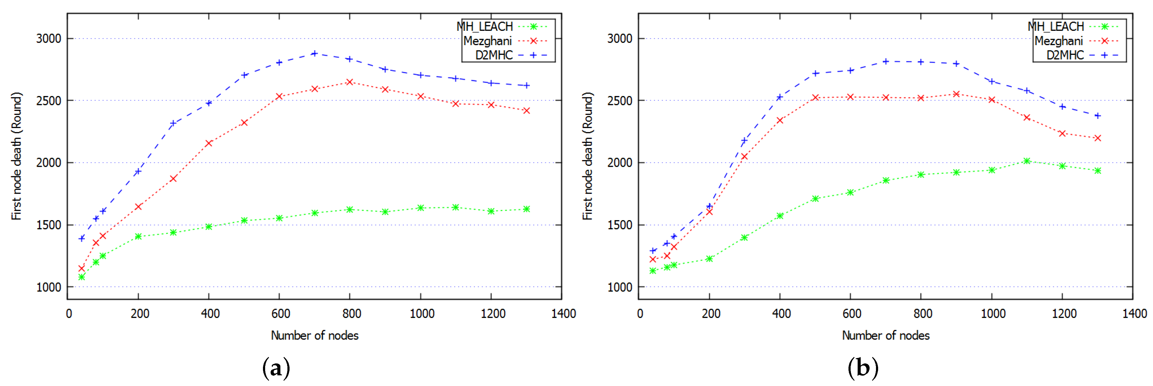
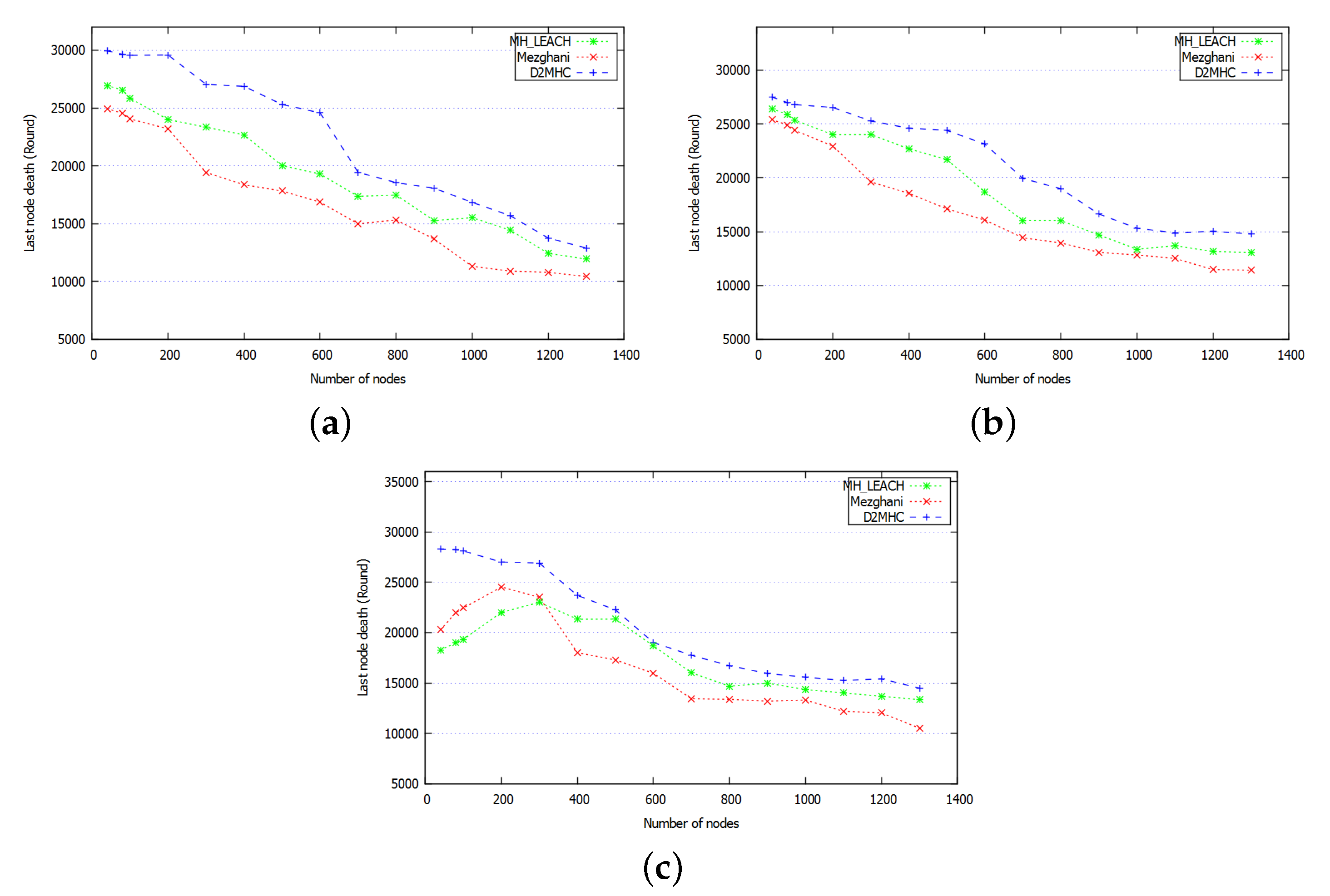
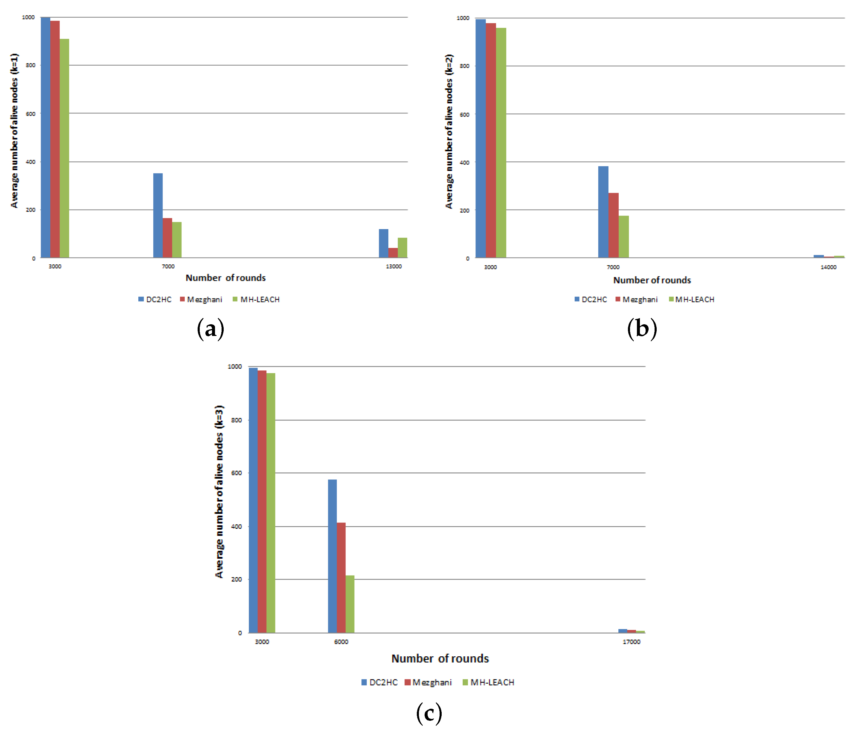
8.2.3. Average Network Lifetime
9. Conclusions and Future Works
Author Contributions
Funding
Institutional Review Board Statement
Informed Consent Statement
Data Availability Statement
Conflicts of Interest
References
- Atzori, L.; Iera, A.; Morabito, G. The internet of things: A survey. Comput. Netw. 2010, 54, 2787–2805. [Google Scholar] [CrossRef]
- Al-Fuqaha, A.; Guizani, M.; Mohammadi, M.; Aledhari, M.; Ayyash, M. Internet of things: A survey on enabling technologies, protocols, and applications. IEEE Commun. Surv. Tutor. 2015, 17, 2347–2376. [Google Scholar] [CrossRef]
- Siow, E.; Tiropanis, T.; Hall, W. Analytics for the internet of things: A survey. ACM Comput. Surv. (CSUR) 2018, 51, 1–36. [Google Scholar] [CrossRef] [Green Version]
- Sethi, P.; Sarangi, S. Internet of Things: Architectures, Protocols, and Applications. J. Electr. Comput. Eng. 2017, 2017, 1–25. [Google Scholar] [CrossRef] [Green Version]
- Sadek, R. Hybrid energy aware clustered protocol for IoT heterogeneous network. Future Comput. Inf. J. 2018, 3, 166–177. [Google Scholar] [CrossRef]
- Liaqat, M.; Gani, A.; Anisi, M.; Ab Hamid, S.; Akhunzada, A.; Khan, M.; Ali, R. Distance-based and low energy adaptive clustering protocol for wireless sensor networks. PLoS ONE 2016, 11, 1–29. [Google Scholar] [CrossRef] [Green Version]
- Toor, A.; Jain, A. Energy aware cluster based multi-hop energy efficient routing protocol using multiple mobile nodes (MEACBM) in wireless sensor networks. AEU-Int. J. Electron. Commun. 2019, 102, 41–53. [Google Scholar] [CrossRef]
- Rostami, A.; Badkoobe, M.; Mohanna, F.; Hosseinabadi, A.; Sangaiah, A.; Sangaiah, A.K. Survey on clustering in heterogeneous and homogeneous wireless sensor networks. J. Supercomput. 2018, 74, 277–323. [Google Scholar] [CrossRef]
- Sert, S.; Alchihabi, A.; Yazici, A. A two-tier distributed fuzzy logic based protocol for efficient data aggregation in multihop wireless sensor networks. IEEE Trans. Fuzzy Syst. 2018, 26, 3615–3629. [Google Scholar] [CrossRef]
- Ozger, M.; Alagoz, F.; Akan, O. Clustering in multi-channel cognitive radio ad hoc and sensor networks. IEEE Commun. Mag. 2018, 56, 156–162. [Google Scholar] [CrossRef]
- Batta, M.S.; Harous, S.; Louail, L.; Aliouat, Z. A Distributed TDMA Scheduling Algorithm for Latency Minimization in Internet of Things. In Proceedings of the IEEE International Conference on Electro Information Technology (EIT), Brookings, SD, USA, 20–22 May 2019; pp. 108–113. [Google Scholar]
- Batta, M.S.; Aliouat, Z.; Harous, S. A Distributed Weight-Based TDMA Scheduling Algorithm for Latency Improvement in IoT. In Proceedings of the IEEE 10th Annual Ubiquitous Computing, Electronics & Mobile Communication Conference (UEMCON), New York, NY, USA, 10–12 October 2019; pp. 768–774. [Google Scholar]
- Cengiz, K.; Dag, T. Energy aware multi-hop routing protocol for WSNs. IEEE Access 2018, 6, 2622–2633. [Google Scholar] [CrossRef]
- Singh, S.; Kumar, P.; Singh, J.; Alryalat, M. An energy efficient routing using multi-hop intra clustering technique in WSNs. In Proceedings of the IEEE Region 10 Conference (TENCON), Penang, Malaysia, 5–8 November 2017; pp. 381–386. [Google Scholar]
- Kumaresan, K.; Kalyani, S. Energy efficient cluster based multilevel hierarchical routing for multi-hop wireless sensor network. J. Ambient. Intell. Humaniz. Comput. 2020, 1–10. [Google Scholar] [CrossRef]
- Batta, M.S.; Mabed, H.; Aliouat, Z. Dynamic Clustering Based Energy Optimization for IoT Network. In International Symposium on Modelling and Implementation of Complex Systems; Springer: Berlin/Heidelberg, Germany, 2020; pp. 77–91. [Google Scholar]
- Ahmed, T.; Abdur, M.; Zaman, A.; Amjad, M. A Scalable K-hop Clustering Algorithm for Pseudo linear MANET. Int. J. Comput. Appl. 2018, 180, 62–68. [Google Scholar]
- Batta, M.S.; Aliouat, Z.; Mabed, H.; Harous, S. LTEOC: Long Term Energy Optimization Clustering for Dynamic IoT Networks. In Proceedings of the IEEE 11th Annual Ubiquitous Computing, Electronics & Mobile Communication Conference (UEMCON), New York, NY, USA, 28–31 October 2020. [Google Scholar]
- Turgut, I. Analysing Multi-hop Intra-Cluster Communication in Cluster-Based Wireless Sensor Networks. Nat. Eng. Sci. 2019, 4, 43–51. [Google Scholar]
- Sucasas, V.; Radwan, A.; Marques, H.; Rodriguez, J.; Vahid, S.; Tafazolli, R. A survey on clustering techniques for cooperative wireless networks. Ad. Hoc. Netw. 2016, 47, 53–81. [Google Scholar] [CrossRef]
- Sim, M.; Lim, Y.; Park, S.H.; Dai, L.; Chae, C. Deep learning-based mmWave beam selection for 5G NR/6G with sub-6 GHz channel information: Algorithms and prototype validation. IEEE Access 2020, 8, 51634–51646. [Google Scholar] [CrossRef]
- Kaur, S.; Mir, R. Clustering in wireless sensor networks-a survey. Int. J. Comput. Netw. Inf. Secur. 2016, 8, 38. [Google Scholar] [CrossRef] [Green Version]
- Meka, S.; Fonseca, B. Improving route selections in ZigBee wireless sensor networks. Sensors 2020, 20, 164. [Google Scholar] [CrossRef] [Green Version]
- Maass, A.; Nevsic, D.; Postoyan, R.; Dower, P. Lp stability of networked control systems implemented on WirelessHART. Automatica 2019, 109, 108514. [Google Scholar] [CrossRef] [Green Version]
- Bouaziz, M.; Rachedi, A. A survey on mobility management protocols in Wireless Sensor Networks based on 6LoWPAN technology. Comput. Commun. 2016, 74, 3–15. [Google Scholar] [CrossRef] [Green Version]
- Yassein, M.; Mardini, W.; Khalil, A. Smart homes automation using Z-wave protocol. In Proceedings of the International Conference on Engineering & MIS (ICEMIS), Agadir, Morocco, 22–24 September 2016; pp. 1–6. [Google Scholar]
- Xu, L.; O’Hare, G.M.; Collier, R. A smart and balanced energy-efficient multihop clustering algorithm (smart-beem) for mimo iot systems in future networks. Sensors 2017, 17, 1574. [Google Scholar] [CrossRef] [PubMed] [Green Version]
- Molina-Masegosa, R.; Gozalvez, J.; Sepulcre, M. Comparison of IEEE 802.11 p and LTE-V2X: An Evaluation With Periodic and Aperiodic Messages of Constant and Variable Size. IEEE Access 2020, 8, 121526–121548. [Google Scholar] [CrossRef]
- Lauridsen, M.; Kovacs, I.; Mogensen, P.; Sorensen, M.; Holst, S. Coverage and capacity analysis of LTE-M and NB-IoT in a rural area. In Proceedings of the IEEE 84th Vehicular Technology Conference (VTC-Fall), Montreal, QC, Canada, 18–21 September 2016; pp. 1–5. [Google Scholar]
- Sinha, R.; Wei, Y.; Hwang, S. A survey on LPWA technology: LoRa and NB-IoT. ICT Express 2017, 3, 14–21. [Google Scholar] [CrossRef]
- Darroudi, S.M.; Gomez, C. Bluetooth low energy mesh networks: A survey. Sensors 2017, 17, 1467. [Google Scholar] [CrossRef] [PubMed] [Green Version]
- Chiani, M.; Elzanaty, A. On the LoRa modulation for IoT: Waveform properties and spectral analysis. IEEE Internet Things J. 2019, 6, 8463–8470. [Google Scholar] [CrossRef] [Green Version]
- Sung, Y.; Lee, S.; Lee, M. A Multi-Hop Clustering Mechanism for Scalable IoT Networks. Sensors 2018, 18, 961. [Google Scholar] [CrossRef] [Green Version]
- Mezghani, M. An efficient multi-hops clustering and data routing for WSNs based on Khalimsky shortest paths. J. Ambient. Intell. Humaniz. Comput. 2019, 10, 1275–1288. [Google Scholar] [CrossRef]
- Elhoseny, M.; Farouk, A.; Zhou, N.; Wang, M.M.; Abdalla, S.; Batle, J. Dynamic multi-hop clustering in a wireless sensor network: Performance improvement. Wirel. Pers. Commun. 2017, 95, 3733–3753. [Google Scholar] [CrossRef]
- Xu, L.; Collier, R.; O’Hare, G.M. A survey of clustering techniques in WSNs and consideration of the challenges of applying such to 5G IoT scenarios. IEEE Internet Things J. 2017, 4, 1229–1249. [Google Scholar] [CrossRef]
- Dehkordi, S.; Farajzadeh, K.; Rezazadeh, J.; Farahbakhsh, R.; Sandrasegaran, K.; Dehkordi, M. A survey on data aggregation techniques in IoT sensor networks. Wirel. Netw. 2020, 26, 1243–1263. [Google Scholar] [CrossRef]
- Zanjireh, M.; Larijani, H. A survey on centralised and distributed clustering routing algorithms for WSNs. In Proceedings of the IEEE 81st Vehicular Technology Conference (VTC Spring), Glasgow, UK, 11–14 May 2015; pp. 1–6. [Google Scholar]
- Song, F.; Ai, Z.; Zhang, H.; You, I.; Li, S. Smart Collaborative Balancing for Dependable Network Components in Cyber-Physical Systems. IEEE Trans. Ind. Inf. 2020. [Google Scholar] [CrossRef]
- Al-Janabi, T.A.; Al-Raweshidy, H.S. Optimised clustering algorithm-based centralised architecture for load balancing in IoT network. In Proceedings of the International Symposium on Wireless Communication Systems (ISWCS), Bologna, Italy, 28–31 October 2017; pp. 269–274. [Google Scholar]
- Song, L.; Chai, K.; Chen, Y.; Schormans, J.; Loo, J.; Vinel, A. QoS-aware energy-efficient cooperative scheme for cluster-based IoT systems. IEEE Syst. J. 2017, 11, 1447–1455. [Google Scholar] [CrossRef] [Green Version]
- Li, J.; Silva, B.N.; Diyan, M.; Cao, Z.; Han, K. A clustering based routing algorithm in IoT aware Wireless Mesh Networks. Sustain. Cities Soc. 2018, 40, 657–666. [Google Scholar] [CrossRef]
- Heinzelman, W.; Chandrakasan, A.; Balakrishnan, H. An application-specific protocol architecture for wireless microsensor networks. IEEE Trans. Wirel. Commun. 2002, 1, 660–670. [Google Scholar] [CrossRef] [Green Version]
- Xiao, M.; Zhang, X.; Dong, Y. An effective routing protocol for energy harvesting wireless sensor networks. In Proceedings of the IEEE Wireless Communications and Networking Conference (WCNC), Shanghai, China, 7–10 April 2013; pp. 2080–2084. [Google Scholar]
- Nayak, P.; Devulapalli, A. A fuzzy logic-based clustering algorithm for WSN to extend the network lifetime. IEEE Sens. J. 2015, 16, 137–144. [Google Scholar] [CrossRef]
- Ammar, A.; Dziri, A.; Terre, M.; Youssef, H. Multi-hop LEACH based cross-layer design for large scale wireless sensor networks. In Proceedings of the International wireless communications and mobile computing conference (IWCMC), Paphos, Cyprus, 5–9 September 2016; pp. 763–768. [Google Scholar]
- Wu, C.; Chiang, T.; Fu, L. An ant colony optimization algorithm for multi-objective clustering in mobile ad hoc networks. In Proceedings of the IEEE Congress on Evolutionary Computation (CEC), Beijing, China, 6–11 July 2014; pp. 2963–2968. [Google Scholar]
- Ghosh, S.; Mondal, S.; Biswas, U. Enhanced PEGASIS using ant colony optimization for data gathering in WSN. In Proceedings of the International Conference on Information Communication and Embedded Systems (ICICES), Chennai, India, 25–26 February 2016; pp. 1–6. [Google Scholar]
- Albath, J.; Thakur, M.; Madria, S. Energy constraint clustering algorithms for wireless sensor networks. Ad Hoc Netw. 2013, 11, 2512–2525. [Google Scholar] [CrossRef]
- Deshpande, V.; Patil, A. Energy efficient clustering in wireless sensor network using cluster of cluster heads. In Proceedings of the International conference on wireless and optical communications networks (WOCN), Bhopal, India, 26–28 July 2013; pp. 1–5. [Google Scholar]
- Luo, J.; Wu, D.; Pan, C.; Zha, J. Optimal energy strategy for node selection and data relay in WSN-based IoT. Mob. Netw. Appl. 2015, 20, 169–180. [Google Scholar] [CrossRef]
- Addario-Berry, L.; Broutin, N.; Goldschmidt, C.; Miermont, G. The scaling limit of the minimum spanning tree of the complete graph. Ann. Probab. 2017, 45, 3075–3144. [Google Scholar] [CrossRef] [Green Version]
- Abbasi, A.; Younis, M. A survey on clustering algorithms for wireless sensor networks. Comput. Commun. 2007, 30, 2826–2841. [Google Scholar] [CrossRef]
- Neggazi, B.; Guellati, N.; Haddad, M.; Kheddouci, H. Efficient Self-Stabilizing Algorithm for Independent Strong Dominating Sets in Arbitrary Graphs. Int. J. Found. Comput. Sci. 2015, 26, 751–768. [Google Scholar] [CrossRef]
- Xu, L.; O’Grady, M.J.; O’Hare, G.M.; Collier, R. Reliable multihop intra-cluster communication for Wireless Sensor Networks. In Proceedings of the International Conference on Computing, Networking and Communications (ICNC), Honolulu, HI, USA, 3–6 February 2014; pp. 858–863. [Google Scholar]
- Baccour, N.; Kouba, A.; Mottola, L.; Zuniga, M.A.; Youssef, H.; Boano, C.A.; Alves, M. Radio link quality estimation in wireless sensor networks: A survey. ACM Trans. Sens. Netw. (TOSN) 2012, 8, 1–33. [Google Scholar] [CrossRef]
- OMadadhain, J.; Fisher, D.; Smyth, P.; White, S.; Boey, Y. Analysis and visualization of network data using JUNG. J. Stat. Softw. 2005, 10, 1–35. [Google Scholar]
- Kim, D.; Jung, M. Data transmission and network architecture in long range low power sensor networks for IoT. Wirel. Pers. Commun. 2017, 93, 119–129. [Google Scholar] [CrossRef]
- Schmid, S.; Wattenhofer, R. Algorithmic models for sensor networks. In Proceedings of the IEEE International Parallel Distributed Processing Symposium (IPDPS), Rhodes Island, Greece, 25–29 April 2006; pp. 450–461. [Google Scholar]
- Li, X.; Wang, Z.; Zhang, L.; Zou, C.; Dorrell, D. State-of-health estimation for Li-ion batteries by combing the incremental capacity analysis method with grey relational analysis. J. Power Sources 2019, 410, 106–114. [Google Scholar] [CrossRef]
- Liagkou, V.; Kavvadas, V.; Chronopoulos, S.K.; Tafiadis, D.; Christofilakis, V.; Peppas, K. Attack detection for healthcare monitoring systems using mechanical learning in virtual private networks over optical transport layer architecture. Computation 2019, 7, 24. [Google Scholar] [CrossRef] [Green Version]


| Protocol | Frequency Band | Data Rate | Range | Energy Consumption | Usage Area |
|---|---|---|---|---|---|
| Wi-Fi [28] | 2.4/5.0 GHz | 54 Mb/s | 30 m | Medium | Home entertainment, Industrial |
| Bluetooth [2] | 2.4 GHz | 1 Mb/s | 10 m | Low | Industrial, Traffic management |
| IEEE 802.15.4 [23] | 868−915 MHz/2.4 GHz | 250 kb/s | [10, 100] m | Low | Industrial, Traffic management, Smart home, vehicle monitoring |
| LTE [29] | 2.6 GHz | 10 Mb/s | ≤15 km | High | Mobil telecommunications, Smart Cities |
| Wireless HART [24] | 2.4−2.5 MHz | 250 kb/s | [1, 100] m | Low | Healthcare, Industry automation |
| BLE [31] | 2.4 MHz | 1 Mb/s | 200 m | Very Low | Healthcare, Home entertainment |
| Z-WAVE [26] | 1 GHz | 40 kb/s | 30 m | Low | Home automation applications |
| WAVENIS [22] | 865−916 GHz | 100 kb/s | ≤4 km | Very Low | Chemical and healthcare applications |
| LoRaWAN [32] | 868−900 GHz | 50 kb/s | ≤15 km | Very Low | Smart City, industrial Monitoring, Agriculture |
| NB-IoT [30] | 180 kHz | 234.7 kb/s | ≤35 km | Low | Industrial Monitoring, Smart City |
| Algorithm | Topology | Number of CH’s | Intra Clustering | Inter Clustering | Load Balancing | Energy Consideration | Benchmarks |
|---|---|---|---|---|---|---|---|
| LEACH [43] | Distributed | Undetermined | Single-hop | Single-hop | No | No | MTE |
| EP-LEACH [44] | Distributed | Undetermined | Single-hop | Single-hop | No | Yes (CH-election) | LEACH, TEEN |
| FL-LEACH [45] | Distributed | Determined | Single-hop | Single-hop | Yes | No | LEACH |
| Wu et al. [47] | Centralized | Undetermined | Single-hop | Single-hop | Yes | No | Not specified |
| MH-LEACH [46] | Distributed | Undetermined | Multi-hop | Single-hop | No | Yes (Multi-Hop transmission) | LEACH |
| E-PEGASIS [48] | Centralized | Determined | Multi-hop | Single-hop | No | No | PEGASIS, LBEERA |
| EE3C [50] | Centralized | Undetermined | Multi-hop | Multi-hop | Yes | No | Not specified |
| K-ECDS [49] | Distributed | Undetermined | Multi-hop | Multi-hop | No | No | ECDS, HEED |
| Singh et al. [14] | Centralized | Undetermined | Multi-hop | Multi-hop | Yes | Yes (CH-rotation) | EEUC, EUCA |
| Turgut [19] | Distributed | Undetermined | Multi-hop | Single-hop | Yes | No | Not specified |
| Mezghani [34] | Distributed | Undetermined | Multi-hop | Single-hop | Yes | Yes (intra-cluster routing) | MTE, HEED, APTEEN, EDC, THC, VCA |
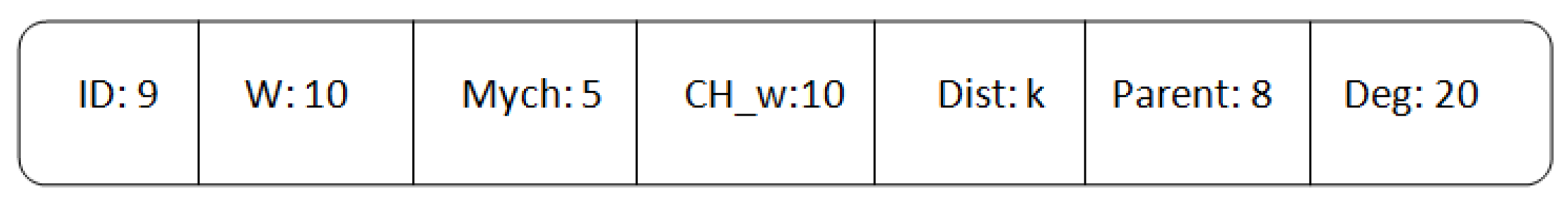
| Symbol | Description |
|---|---|
| Identity of device i | |
| Weight of i (computed using Equation (5)) | |
| Relative Cluster Head of i | |
| Weight of | |
| Distance between i and (in term of hops) | |
| Parent of i in the aggregation path toward the relative CH | |
| Transmitting range of i | |
| Degree of i (Number of node in the neighborhood of i) | |
| Local State Variable of i | |
| Clustering Record List (Neighbors clustering information received) | |
| Two-hop connectivity ration of i |
| Parameter | Value |
|---|---|
| Network size () | 1000 × 1000 m |
| Node density | |
| Distribution of nodes | Random |
| connectivity model | Unit Disk Graph (UDG [59]) |
| Transmitting range () | 70 m |
| Maximum hop constraint k | |
| 1/3, 1/3, 1/3 | |
| 50 nJ/bit | |
| 10 pJ/ bit/ M | |
| 0.0013 pJ/ bit/ M | |
| Data packet size | 100 bytes |
| Initial energy | 1 Joule |
| Clustering Algorithm | Intra-Cluster Topology | ||
|---|---|---|---|
| Single-hop | Two-hop | Three-hop | |
| Mezghani | 6.9% | 21.1% | 27% |
| MH-LEACH | 55.3% | 64.2% | 67.3% |
| Clustering Algorithm | Intra-Cluster Topology | ||
|---|---|---|---|
| Single-hop | Two-hop | Three-hop | |
| Mezghani | 28.7% | 37% | 37.1% |
| MH-LEACH | 10.6% | 13.8% | 3.1% |
| Clustering Algorithm | Intra-Cluster Topology | |||
|---|---|---|---|---|
| FND | LND | |||
| Single-hop | Multi-hop | Single-hop | Multi-hop | |
| Mezghani | 30.5% | 24.2% | 16.4% | 10.2% |
| MH-LEACH | 14.4% | 14.7% | 75.1% | 41.8% |
Publisher’s Note: MDPI stays neutral with regard to jurisdictional claims in published maps and institutional affiliations. |
© 2021 by the authors. Licensee MDPI, Basel, Switzerland. This article is an open access article distributed under the terms and conditions of the Creative Commons Attribution (CC BY) license (http://creativecommons.org/licenses/by/4.0/).
Share and Cite
Batta, M.S.; Mabed, H.; Aliouat, Z.; Harous, S. A Distributed Multi-Hop Intra-Clustering Approach Based on Neighbors Two-Hop Connectivity for IoT Networks. Sensors 2021, 21, 873. https://doi.org/10.3390/s21030873
Batta MS, Mabed H, Aliouat Z, Harous S. A Distributed Multi-Hop Intra-Clustering Approach Based on Neighbors Two-Hop Connectivity for IoT Networks. Sensors. 2021; 21(3):873. https://doi.org/10.3390/s21030873
Chicago/Turabian StyleBatta, Mohamed Sofiane, Hakim Mabed, Zibouda Aliouat, and Saad Harous. 2021. "A Distributed Multi-Hop Intra-Clustering Approach Based on Neighbors Two-Hop Connectivity for IoT Networks" Sensors 21, no. 3: 873. https://doi.org/10.3390/s21030873