Laser-Based People Detection and Obstacle Avoidance for a Hospital Transport Robot


Abstract
:1. Introduction
- The behavior produced should be legible and predictable by humans, to improve navigation efficiency and avoid dangerous people reactions [24];
- The trajectory generated by the local planner should lead to the target point.
2. Related Work
2.1. People Detection in Laser Data
2.2. Local Obstacle Avoidance
3. System Overview
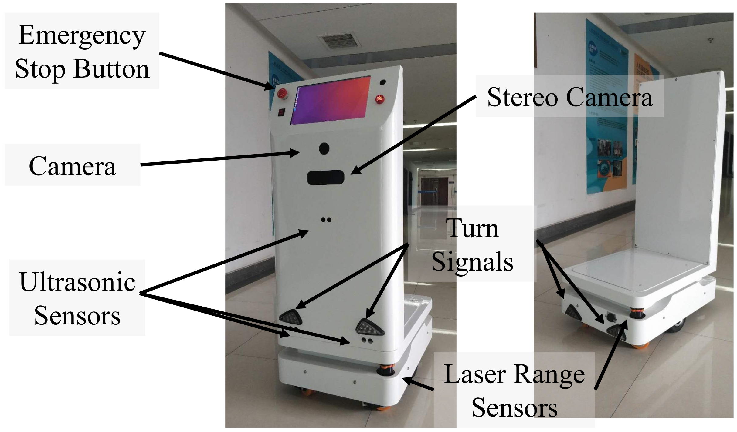
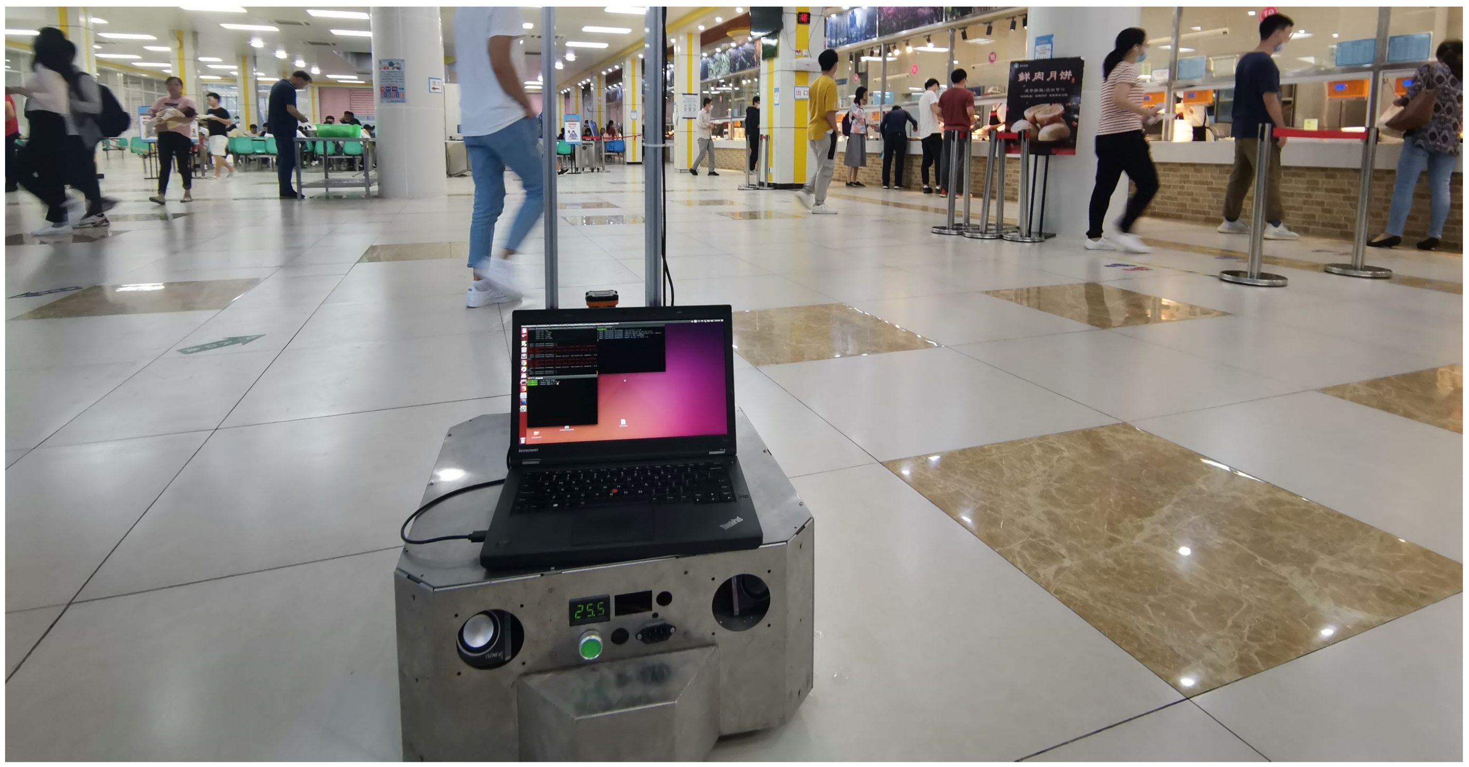
3.1. Robot Design
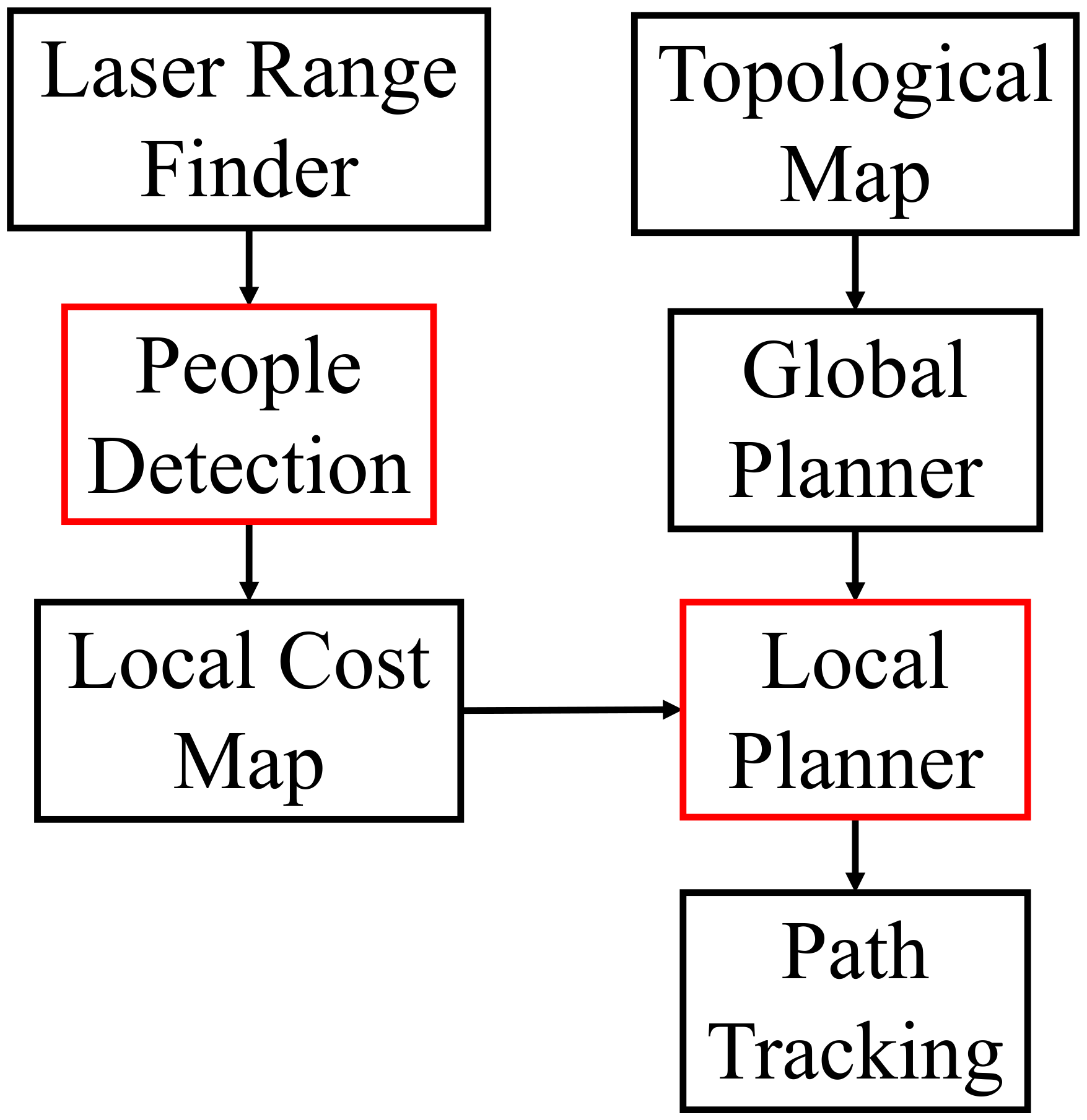
3.2. System Architecture
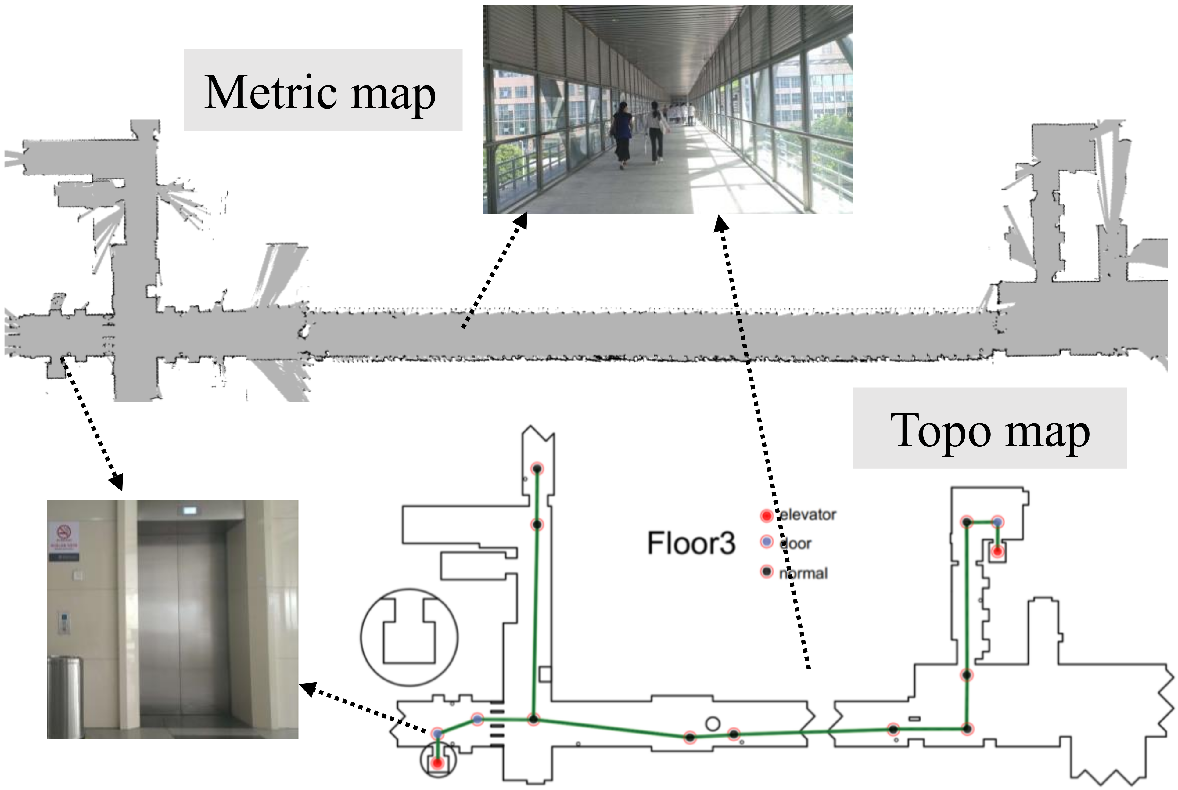
3.3. Maps
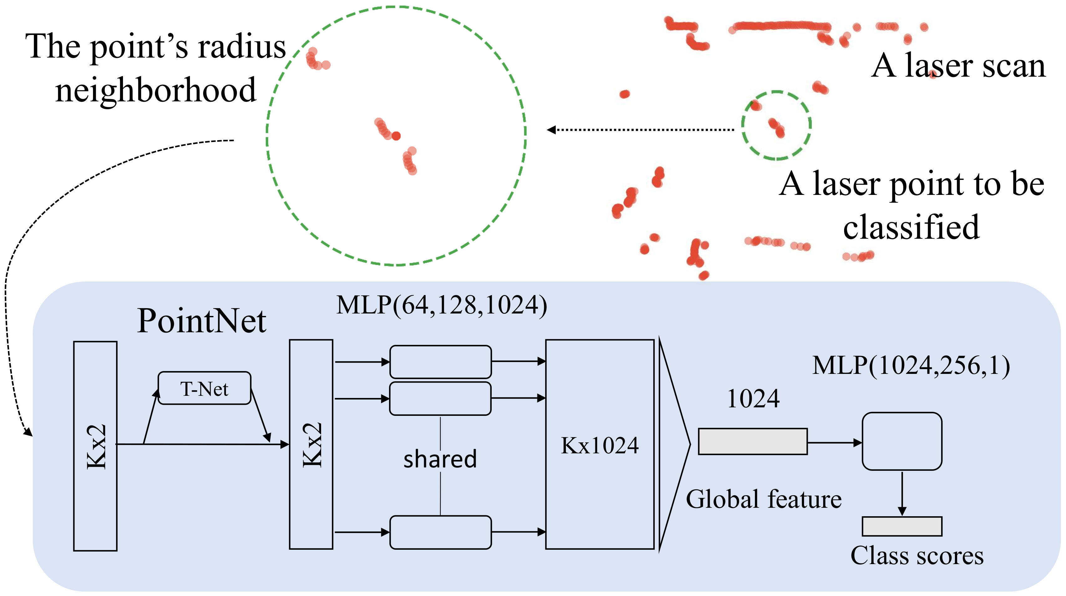
4. People Detection
4.1. Preprocessing
4.2. Inputs
4.3. Network
4.4. Inference
4.5. Automated Dataset Annotation
| Algorithm 1 Automated Annotation of Laser Scans |
| Require: set of laser scans Ensure: set of labels of laser scans
|
| Algorithm 2 Projection of laser points to a grid map |
| Require: filtered laser points Ensure: grid map M
|
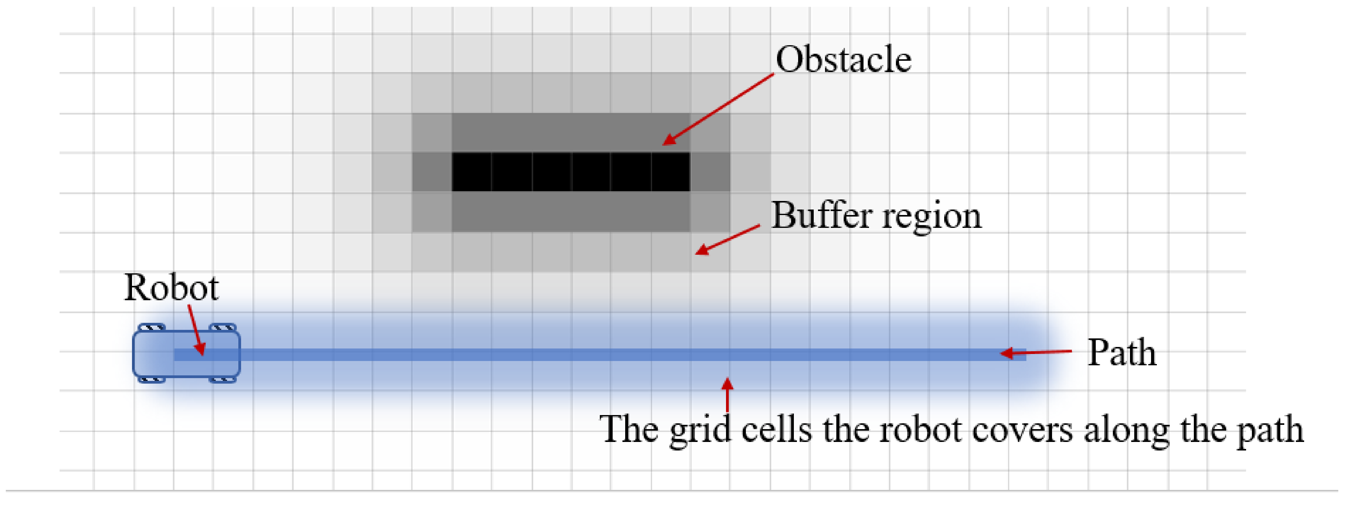
5. Obstacle Avoidance
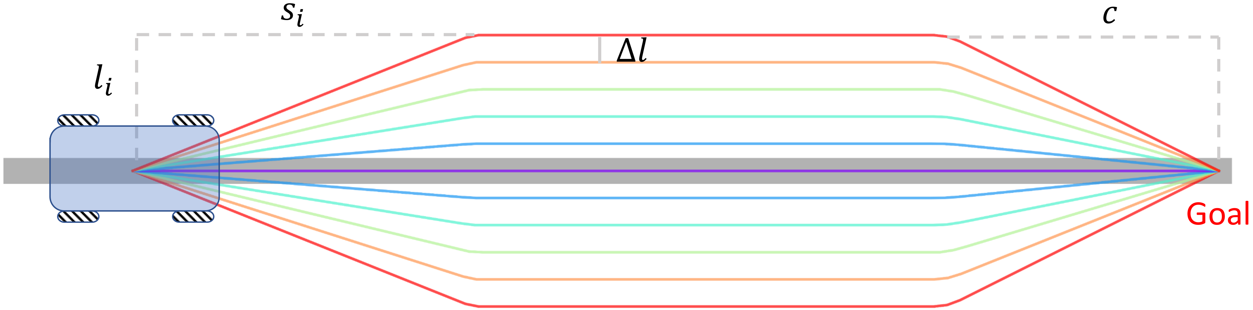
5.1. Generation of Candidate Paths
5.2. Path Selection
5.3. Behavior States
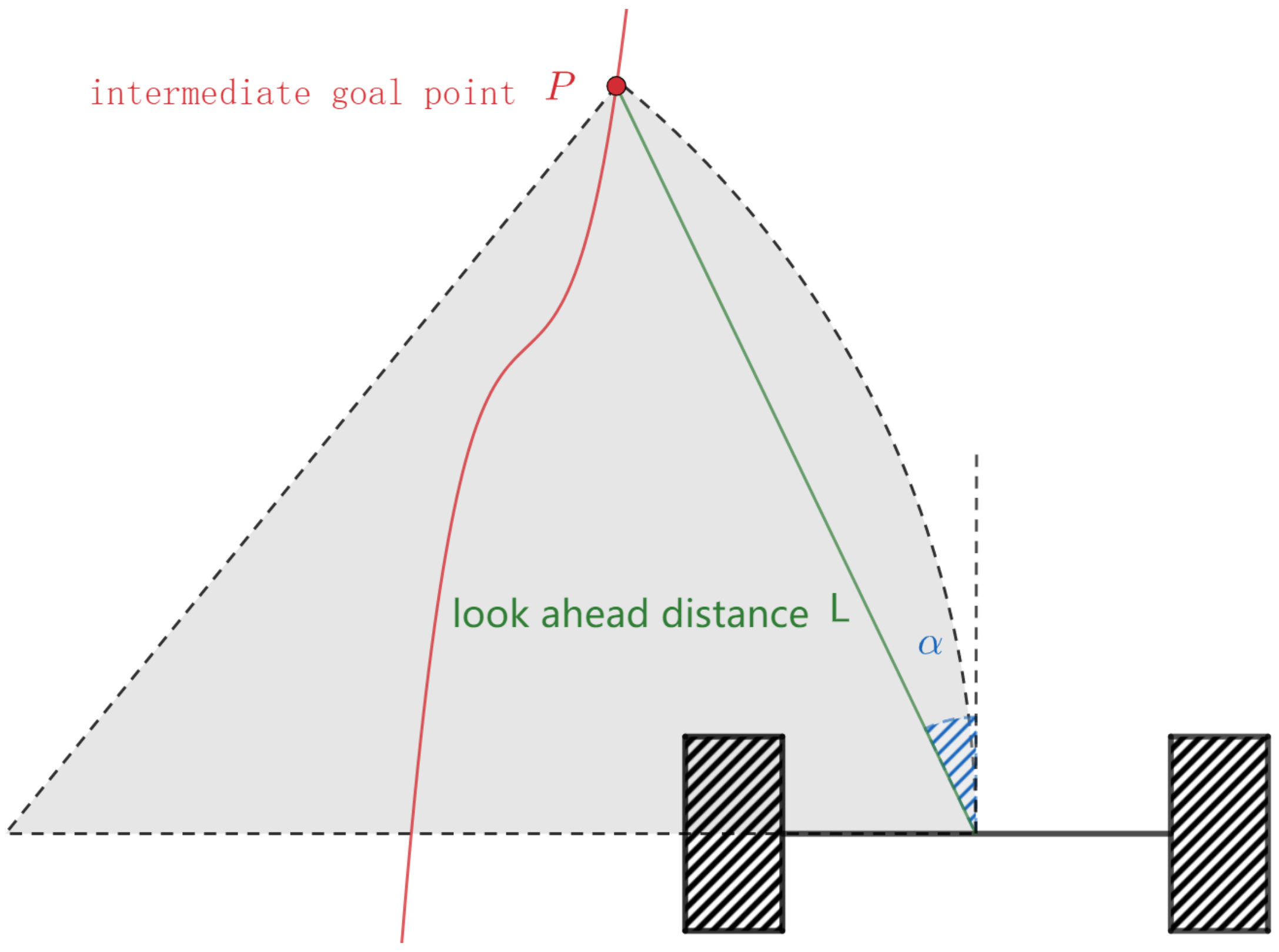
5.4. Path Tracking
6. Experimental Evaluation
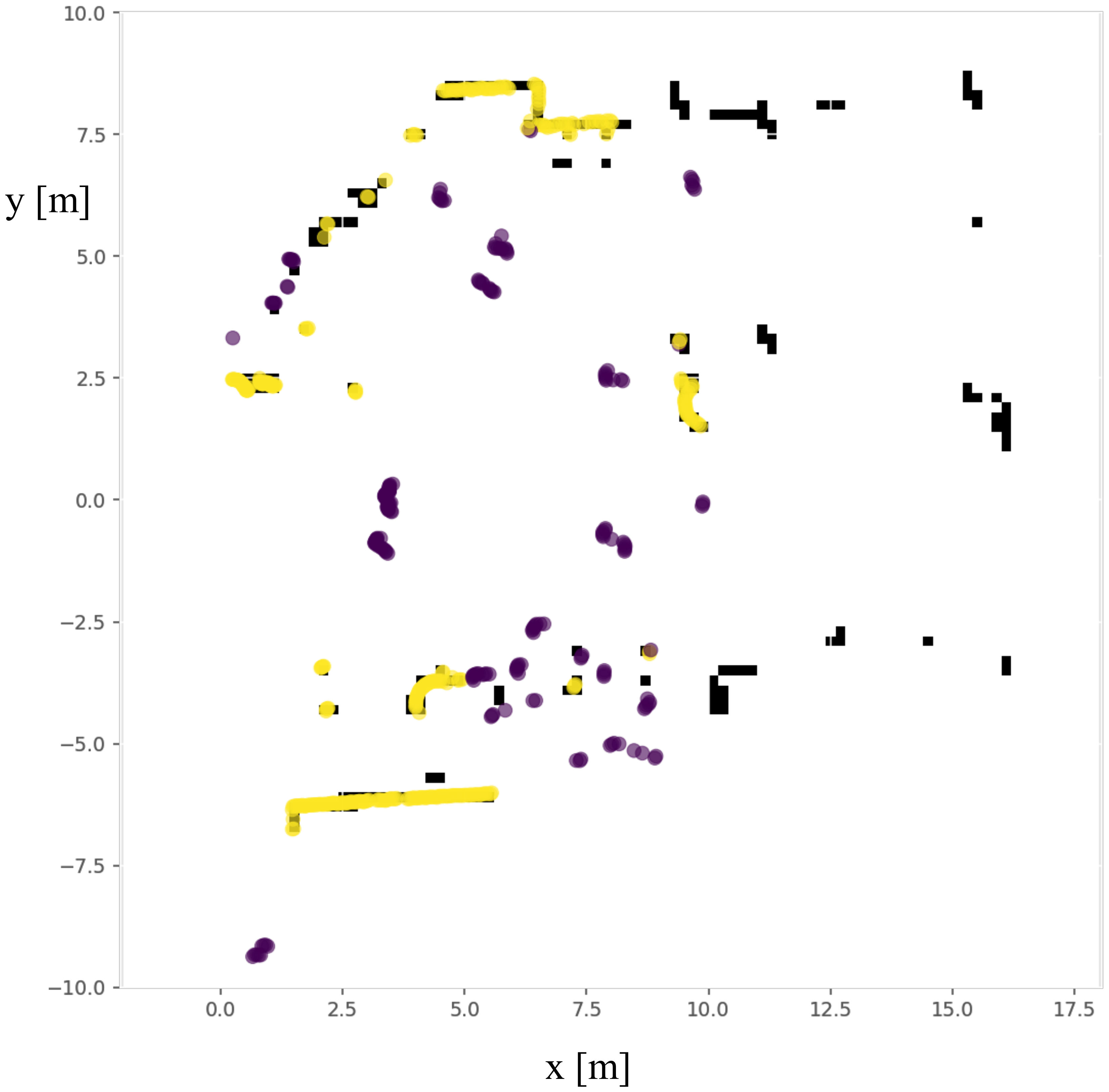
6.1. Experiments on People Detection
6.1.1. Dataset
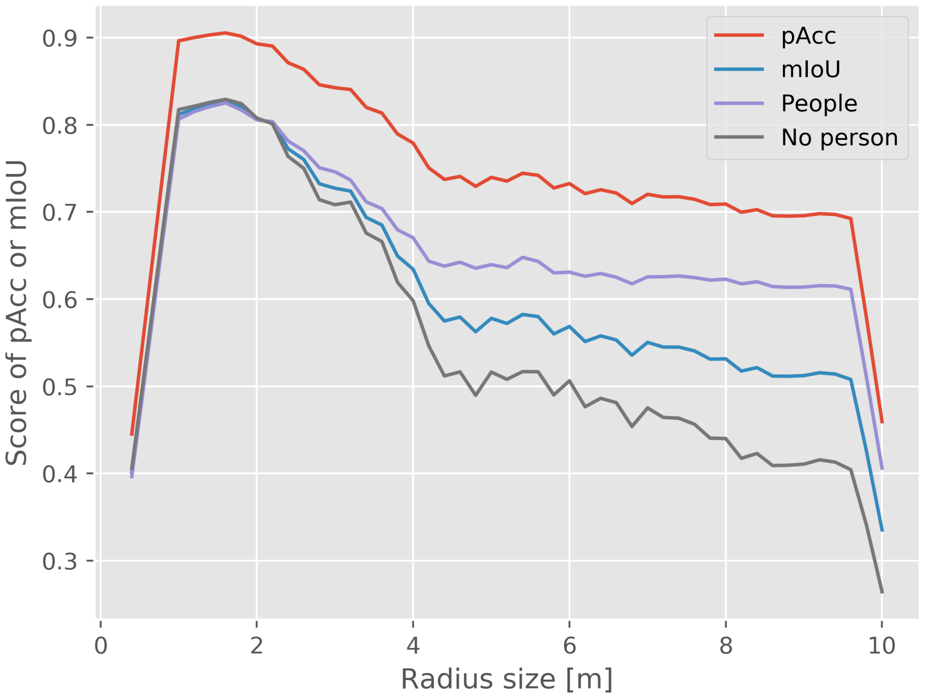
6.1.2. Radius Size
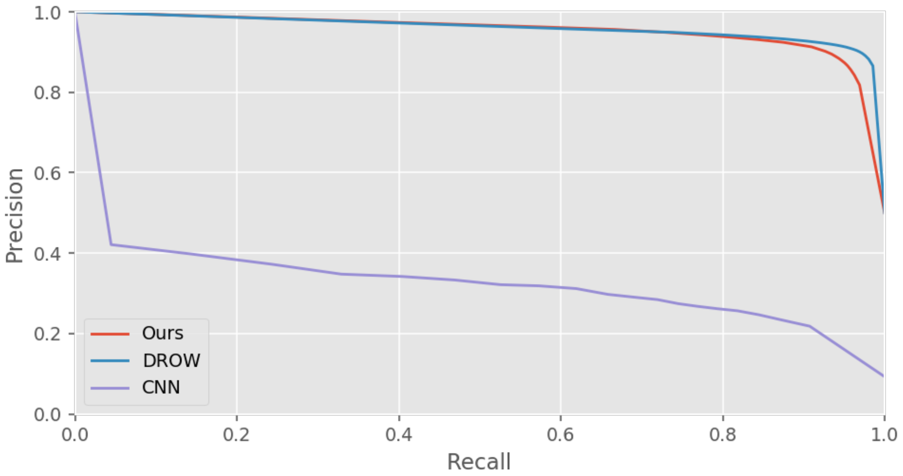
6.1.3. Baselines
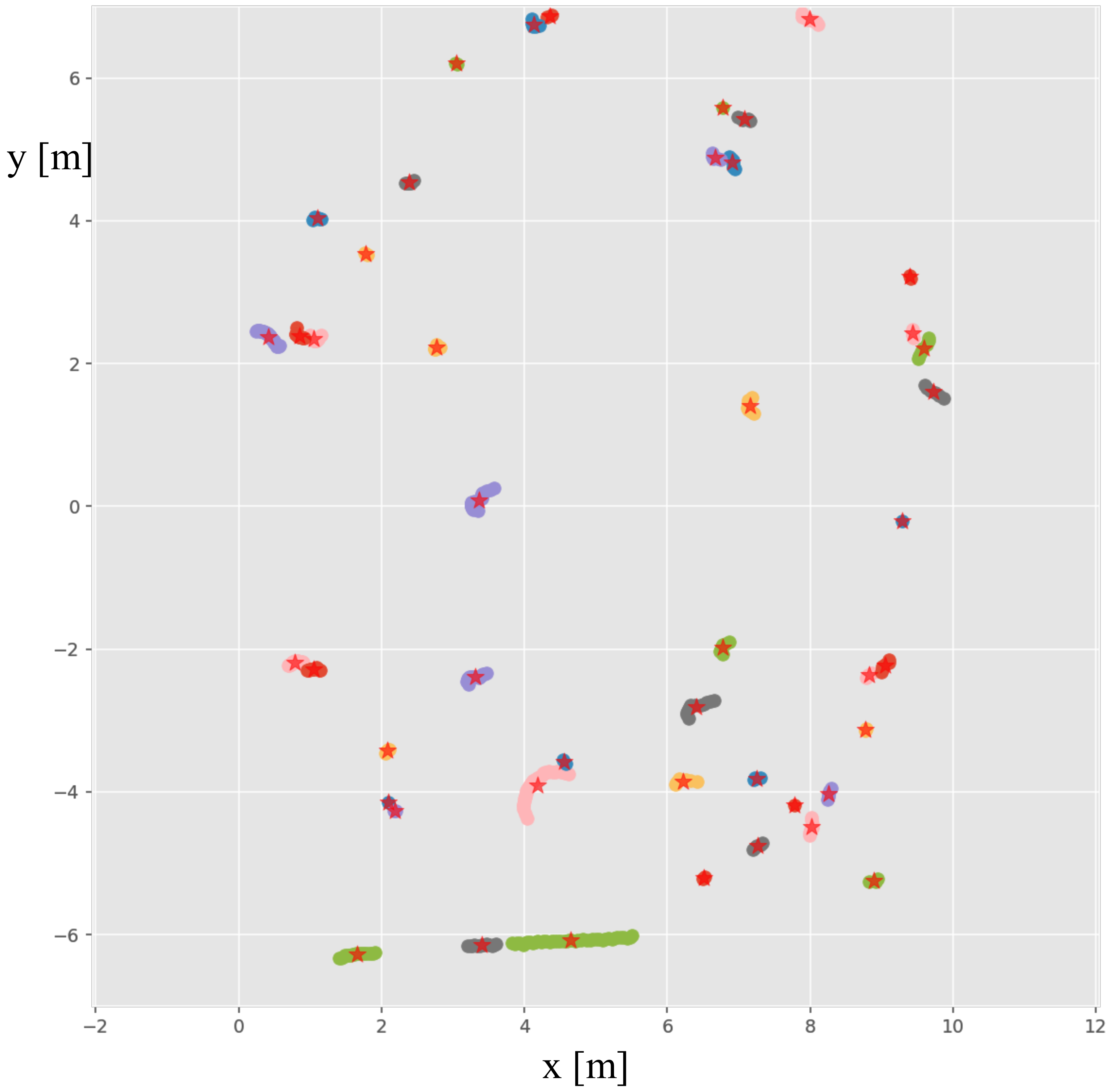
6.1.4. Results
6.2. Experiments on Obstacle Avoidance
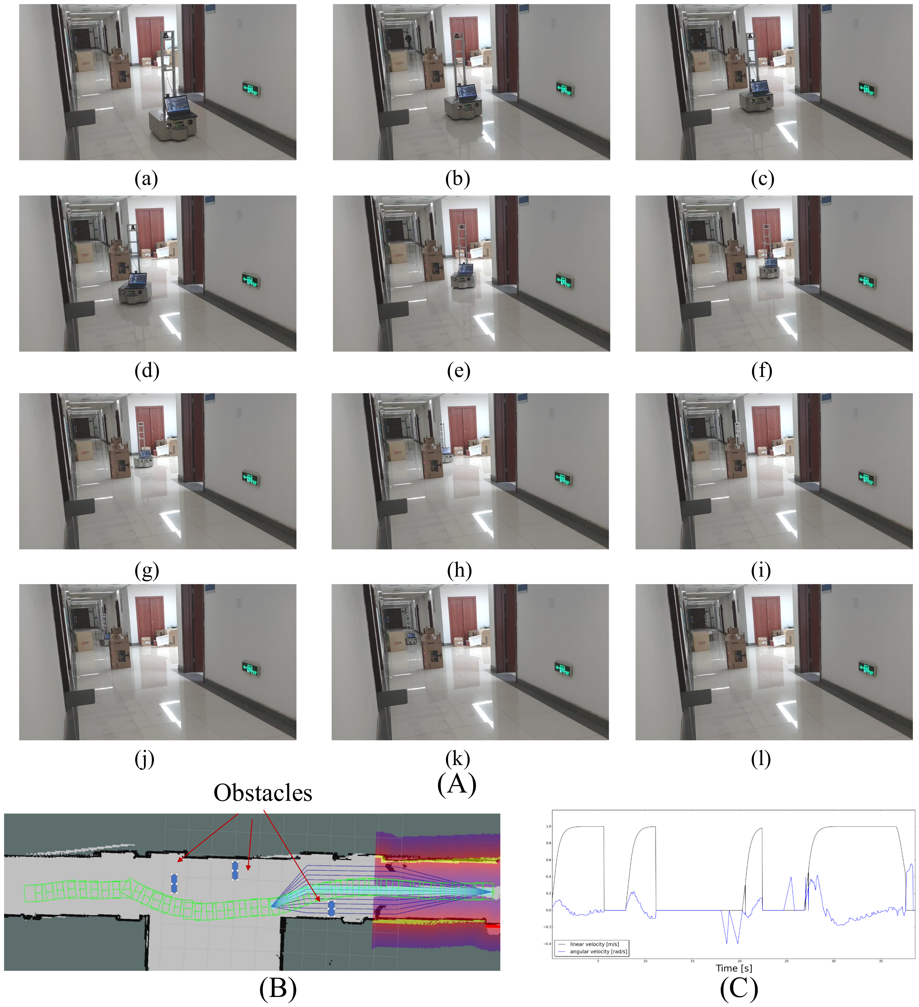
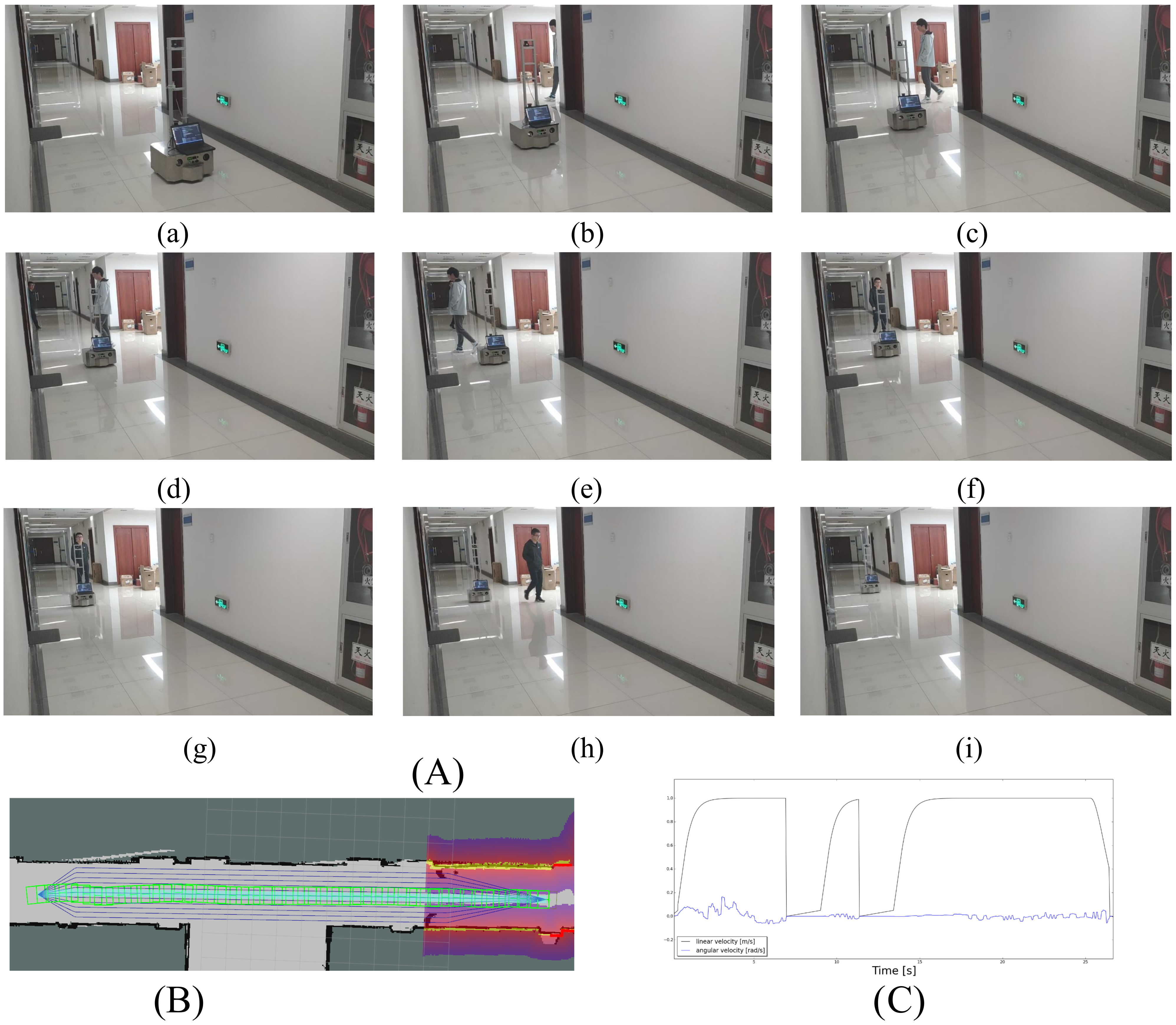
6.2.1. Case 1: Static Obstacles
6.2.2. Case 2: Crossing Scenarios
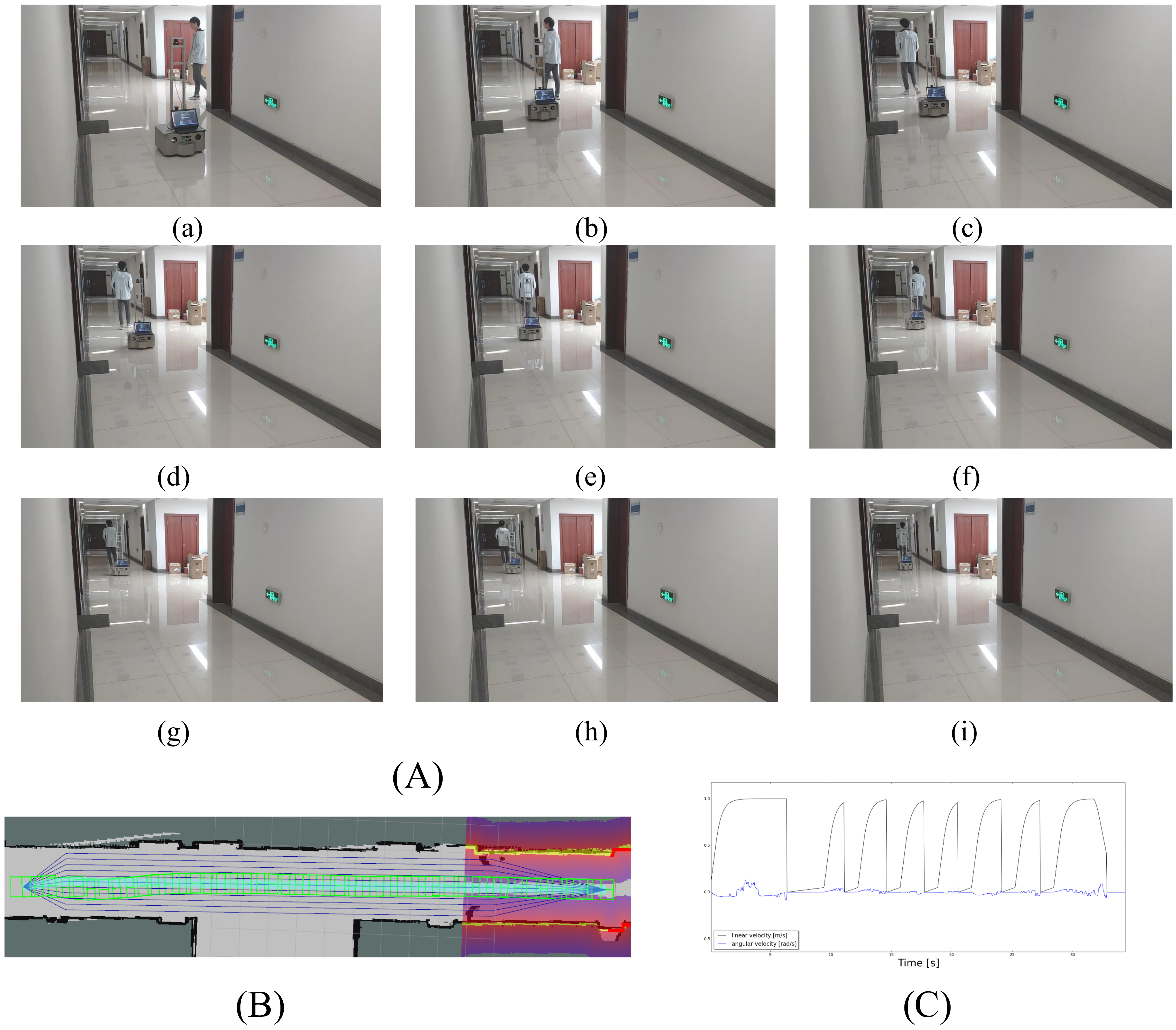
6.2.3. Case 3: Following a Person
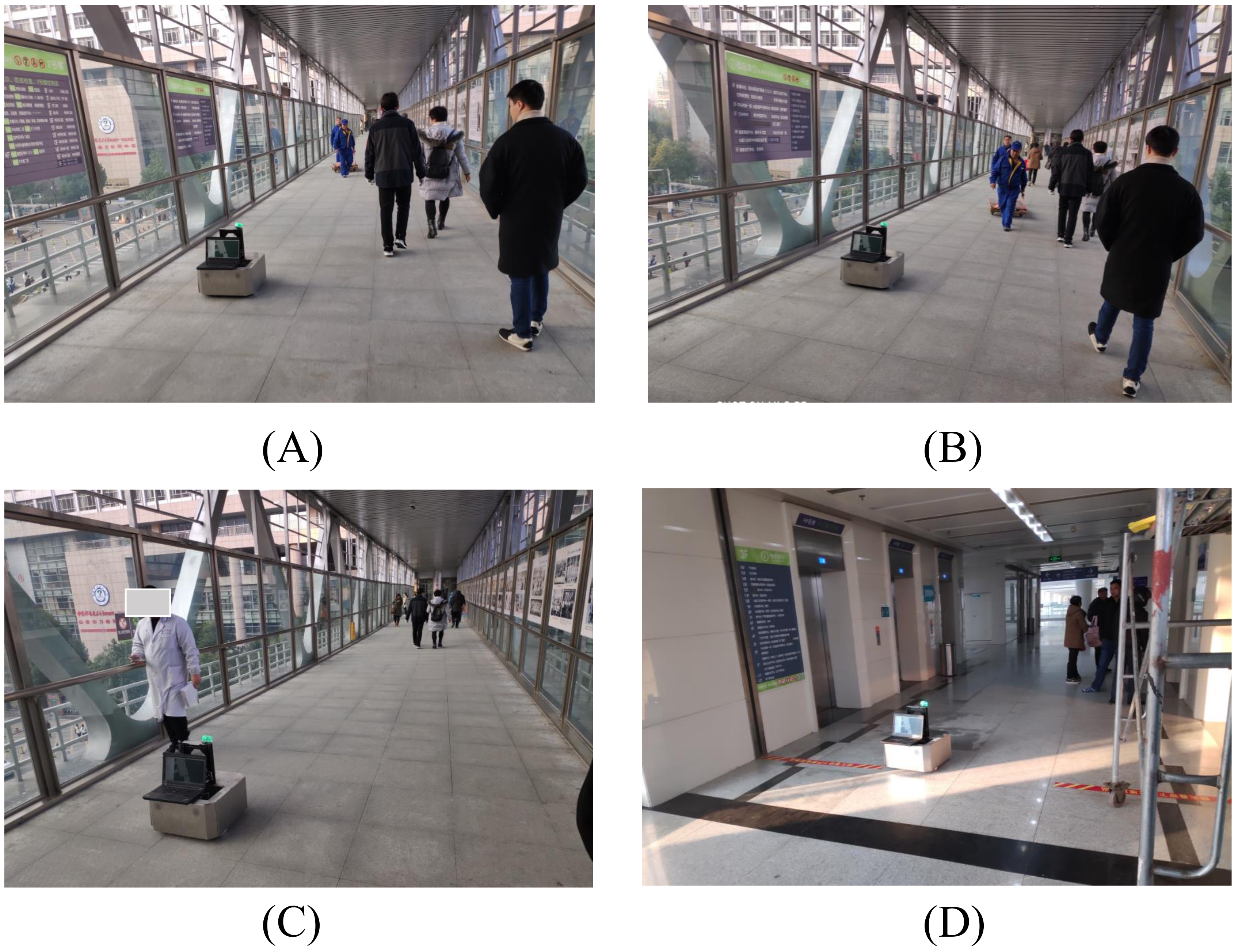
6.3. Experimental Results in the Hospital
7. Conclusions
Author Contributions
Funding
Conflicts of Interest
References
- Ozkil, A.G.; Fan, Z.; Dawids, S.; Aanes, H.; Kristensen, J.K.; Christensen, K.H. Service Robots for Hospitals: A Case Study of Transportation Tasks in a Hospital. In Proceedings of the 2009 IEEE International Conference on Automation and Logistics, Shenyang, China, 5–7 August 2009; pp. 289–294. [Google Scholar] [CrossRef] [Green Version]
- Niechwiadowicz, K.; Khan, Z. Robot Based Logistics System for Hospitals—Survey. In Proceedings of the IDT Workshop on Interesting Results in Computer Science and Engineering, Vasteras, Sweden, October 2008. [Google Scholar]
- Rossetti, M.; Kumar, A.; Felder, R. Mobile Robot Simulation of Clinical Laboratory Deliveries. In 1998 Winter Simulation Conference Proceedings (Cat. No.98CH36274); IEEE: Washington, DC, USA, 1998; Volume 2, pp. 1415–1422. [Google Scholar] [CrossRef] [Green Version]
- Bacik, J.; Durovsky, F.; Biros, M.; Kyslan, K.; Perdukova, D.; Padmanaban, S. Pathfinder–Development of Automated Guided Vehicle for Hospital Logistics. IEEE Access 2017, 5, 26892–26900. [Google Scholar] [CrossRef]
- Acosta Calderon, C.A.; Mohan, E.R.; Ng, B.S. Development of a Hospital Mobile Platform for Logistics Tasks. Digit. Commun. Network 2015, 1, 102–111. [Google Scholar] [CrossRef] [Green Version]
- Evans, J.; Krishnamurthy, B.; Barrows, B.; Skewis, T.; Lumelsky, V. Handling Real-World Motion Planning: A Hospital Transport Robot. IEEE Control Syst. Mag. 1992, 12, 15–19. [Google Scholar]
- Carreira, F.; Canas, T.; Silva, A.; Cardeira, C. I-Merc: A Mobile Robot to Deliver Meals inside Health Services. In Proceedings of the 2006 IEEE Conference on Robotics, Automation and Mechatronics, Bangkok, Thailand, 21–24 September 2006; pp. 1–8. [Google Scholar] [CrossRef]
- Takahashi, M.; Suzuki, T.; Shitamoto, H.; Moriguchi, T.; Yoshida, K. Developing a Mobile Robot for Transport Applications in the Hospital Domain. Robot. Auton. Syst. 2010, 58, 889–899. [Google Scholar] [CrossRef]
- Mozos, O.M.; Kurazume, R.; Hasegawa, T. Multi-Part People Detection Using 2D Range Data. Int. J. Soc. Robot. 2010, 2, 31–40. [Google Scholar] [CrossRef]
- Kim, B.; Choi, B.; Park, S.; Kim, H.; Kim, E. Pedestrian/Vehicle Detection Using a 2.5-D Multi-Layer Laser Scanner. IEEE Sens. J. 2016, 16, 400–408. [Google Scholar] [CrossRef]
- Gidel, S.; Checchin, P.; Blanc, C.; Chateau, T.; Trassoudaine, L. Pedestrian Detection and Tracking in Urban Environment Using a Multilayer Laserscanner; IEEE: Piscatway, NJ, USA, 2010; p. 12. [Google Scholar]
- Arras, K.O.; Mozos, O.M.; Burgard, W. Using Boosted Features for the Detection of People in 2D Range Data. In Proceedings of the 2007 IEEE International Conference on Robotics and Automation, Rome, Italy, 10–14 April 2007; pp. 3402–3407. [Google Scholar] [CrossRef] [Green Version]
- Weinrich, C.; Wengefeld, T.; Schroeter, C.; Gross, H.M. People Detection and Distinction of Their Walking Aids in 2D Laser Range Data Based on Generic Distance-Invariant Features. In Proceedings of the 23rd IEEE International Symposium on Robot and Human Interactive Communication, Edinburgh, UK, 29–31 August 2014; pp. 767–773. [Google Scholar] [CrossRef]
- Leigh, A.; Pineau, J.; Olmedo, N.; Zhang, H. Person Tracking and Following with 2D Laser Scanners. In Proceedings of the 2015 IEEE International Conference on Robotics and Automation (ICRA), Seattle, WA, USA, 26–30 May 2015; pp. 726–733. [Google Scholar] [CrossRef] [Green Version]
- Spinello, L.; Siegwart, R. Human Detection Using Multimodal and Multidimensional Features. In Proceedings of the 2008 IEEE International Conference on Robotics and Automation, Pasadena, CA, USA, 19–23 May 2008; pp. 3264–3269. [Google Scholar] [CrossRef] [Green Version]
- Mendes, A.; Bento, L.; Nunes, U. Multi-Target Detection and Tracking with a Laserscanner. In Proceedings of the IEEE Intelligent Vehicles Symposium, Parma, Italy, 14–17 June 2004; pp. 796–801. [Google Scholar] [CrossRef]
- Gidel, S.; Checchin, P.; Blanc, C.; Chateau, T.; Trassoudaine, L. Pedestrian Detection Method Using a Multilayer Laserscanner: Application in Urban Environment. In Proceedings of the 2008 IEEE/RSJ International Conference on Intelligent Robots and Systems, Nice, France, 22–26 September 2008; pp. 173–178. [Google Scholar] [CrossRef]
- Spinello, L.; Arras, K.O.; Triebel, R.; Siegwart, R. A Layered Approach to People Detection in 3D Range Data. In Proceedings of the Twenty-Fourth AAAI Conference on Artificial Intelligence AAAI’10, Atlanta, GA, USA, 11–15 July 2010; pp. 1625–1630. [Google Scholar]
- Beyer, L.; Hermans, A.; Leibe, B. DROW: Real-Time Deep Learning-Based Wheelchair Detection in 2-D Range Data. IEEE Robot. Autom. Lett. 2017, 2, 585–592. [Google Scholar] [CrossRef] [Green Version]
- Beyer, L.; Hermans, A.; Linder, T.; Arras, K.O.; Leibe, B. Deep Person Detection in 2D Range Data. arXiv 2018, arXiv:1804.02463[cs]. [Google Scholar]
- Qi, C.R.; Su, H.; Mo, K.; Guibas, L.J. PointNet: Deep Learning on Point Sets for 3D Classification and Segmentation. arXiv 2017, arXiv:1612.00593[cs]. [Google Scholar]
- Lu, D.V.; Hershberger, D.; Smart, W.D. Layered Costmaps for Context-Sensitive Navigation. In Proceedings of the 2014 IEEE/RSJ International Conference on Intelligent Robots and Systems, Chicago, IL, USA, 14–18 September 2014; pp. 709–715. [Google Scholar] [CrossRef]
- Kruse, T.; Pandey, A.K.; Alami, R.; Kirsch, A. Human-Aware Robot Navigation: A Survey. Robot. Auton. Syst. 2013, 61, 1726–1743. [Google Scholar] [CrossRef] [Green Version]
- Bassani, C.; Scalmato, A.; Mastrogiovanni, F.; Sgorbissa, A. Towards an Integrated and Human-Friendly Path Following and Obstacle Avoidance Behaviour for Robots. In Proceedings of the 2016 25th IEEE International Symposium on Robot and Human Interactive Communication (RO-MAN), New York, NY, USA, 26–31 August 2016; pp. 599–605. [Google Scholar] [CrossRef]
- Sgorbissa, A.; Zaccaria, R. Roaming Stripes: Smooth Reactive Navigation in a Partially Known Environment. In Proceedings of the 12th IEEE International Workshop on Robot and Human Interactive Communication, Millbrae, CA, USA, 2 November 2003; pp. 19–24. [Google Scholar] [CrossRef]
- Sgorbissa, A.; Zaccaria, R. Planning and Obstacle Avoidance in Mobile Robotics. Robot. Auton. Syst. 2012, 60, 628–638. [Google Scholar] [CrossRef]
- Thrun, S.; Montemerlo, M.; Dahlkamp, H.; Stavens, D.; Aron, A.; Diebel, J.; Fong, P.; Gale, J.; Halpenny, M.; Hoffmann, G.; et al. Stanley: The Robot That Won the DARPA Grand Challenge. J. Field Robot. 2006, 23, 661–692. [Google Scholar] [CrossRef]
- Howard, T.M.; Green, C.J.; Kelly, A.; Ferguson, D. State Space Sampling of Feasible Motions for High-Performance Mobile Robot Navigation in Complex Environments. J. Field Robot. 2008, 25, 325–345. [Google Scholar] [CrossRef]
- Li, X.; Sun, Z.; Kurt, A.; Zhu, Q. A Sampling-Based Local Trajectory Planner for Autonomous Driving along a Reference Path. In Proceedings of the 2014 IEEE Intelligent Vehicles Symposium Proceedings, Dearborn, MI, USA, 8–11 June 2014; pp. 376–381. [Google Scholar] [CrossRef]
- Darweesh, H.; Takeuchi, E.; Takeda, K.; Ninomiya, Y.; Sujiwo, A.; Morales, L.Y.; Akai, N.; Tomizawa, T.; Kato, S. Open Source Integrated Planner for Autonomous Navigation in Highly Dynamic Environments. J. Robot. Mechatron. 2017, 29, 668–684. [Google Scholar] [CrossRef]
- Chu, K.; Lee, M.; Sunwoo, M. Local Path Planning for Off-Road Autonomous Driving With Avoidance of Static Obstacles. IEEE Trans. Intell. Transp. Syst. 2012, 13, 1599–1616. [Google Scholar] [CrossRef]
- Fox, D.; Burgard, W.; Thrun, S. The Dynamic Window Approach to Collision Avoidance. IEEE Robot. Autom. Mag. 1997, 4, 23–33. [Google Scholar] [CrossRef] [Green Version]
- Ulrich, I.; Borenstein, J. VFH*: Local Obstacle Avoidance with Look-Ahead Verification. In Proceedings of the 2000 ICRA, Millennium Conference, IEEE International Conference on Robotics and Automation, San Francisco, CA, USA, 24–28 April 2000; Volume 3, pp. 2505–2511. [Google Scholar]
- Damas, B.; Santos-Victor, J. Avoiding Moving Obstacles: The Forbidden Velocity Map. In Proceedings of the 2009 IEEE/RSJ International Conference on Intelligent Robots and Systems, St. Louis, MO, USA, 10–15 October 2009; pp. 4393–4398. [Google Scholar] [CrossRef]
- Hwang, Y.; Ahuja, N. A Potential Field Approach to Path Planning. IEEE Transact. Robot. Automat. 1992, 8, 23–32. [Google Scholar] [CrossRef] [Green Version]
- Burgard, W.; Cremers, A.B.; Fox, D.; Hähnel, D.; Lakemeyer, G.; Schulz, D.; Steiner, W.; Thrun, S. Experiences with an Interactive Museum Tour-Guide Robot. Artif. Intell. 1999, 53. [Google Scholar] [CrossRef] [Green Version]
- Chen, Y.; Wu, F.; Shuai, W.; Chen, X. Robots Serve Humans in Public Places— KeJia Robot A Shopp. Assist. Int. J. Adv. Robot. Syst. 2017, 14. [Google Scholar] [CrossRef] [Green Version]
- Fung, W.; Leung, Y.; Chow, M.; Liu, Y.; Xu, Y.; Chan, W.; Law, T.; Tso, S.; Wang, C. Development of a Hospital Service Robot for Transporting Task. In Proceedings of the IEEE International Conference on Robotics, Intelligent Systems and Signal Processing, Changsha, Hunan, China, 8–13 October 2003; Volume 1, pp. 628–633. [Google Scholar] [CrossRef]
- Xavier, J.; Pacheco, M.; Castro, D.; Ruano, A.; Nunes, U. Fast Line, Arc/Circle and Leg Detection from Laser Scan Data in a Player Driver. In Proceedings of the 2005 IEEE International Conference on Robotics and Automation, Barcelona, Spain, 14–17 September 2005; pp. 3930–3935. [Google Scholar] [CrossRef] [Green Version]
- Topp, E.; Christensen, H. Tracking for Following and Passing Persons. In Proceedings of the 2005 IEEE/RSJ International Conference on Intelligent Robots and Systems, Edmonton, AL, Canada, 2–6 August 2005; pp. 2321–2327. [Google Scholar] [CrossRef]
- Kleinehagenbrock, M.; Lang, S.; Fritsch, J.; Lomker, F.; Fink, G.; Sagerer, G. Person Tracking with a Mobile Robot Based on Multi-Modal Anchoring. In Proceedings of the 11th IEEE International Workshop on Robot and Human Interactive Communication, Berlin, Germany, 11–14 March 2002; pp. 423–429. [Google Scholar] [CrossRef] [Green Version]
- Fod, A.; Howard, A.; Mataric, M.J. Laser-Based People Tracking. In Proceedings of the IEEE International Conference on Robotics and Automation (ICRA 2002), Washington, DC, USA, 11–15 May 2002; pp. 3024–3029. [Google Scholar]
- Zhao, H.; Shibasaki, R. A Novel System for Tracking Pedestrians Using Multiple Single-Row Laser-Range Scanners. IEEE Trans. Syst. Man. Cybern. Pt. A Syst. Humans 2005, 35, 283–291. [Google Scholar] [CrossRef]
- Schulz, D.; Burgard, W.; Fox, D.; Cremers, A.B. People Tracking with Mobile Robots Using Sample-Based Joint Probabilistic Data Association Filters. Int. J. Robot. Res. 2003, 22, 99–116. [Google Scholar] [CrossRef]
- Schulz, D.; Burgard, W.; Fox, D.; Cremers, A. Tracking Multiple Moving Targets with a Mobile Robot Using Particle Filters and Statistical Data Association. In Proceedings of the 2001 ICRA, IEEE International Conference on Robotics and Automation (Cat. No.01CH37164), Seoul, Korea, 2001; Volume 2, pp. 1665–1670. [Google Scholar] [CrossRef]
- Cui, J.; Zha, H.; Zhao, H.; Shibasaki, R. Laser-Based Detection and Tracking of Multiple People in Crowds. Comput. Vis. Image Underst. 2007, 106, 300–312. [Google Scholar] [CrossRef]
- Chung, W.; Kim, H.; Yoo, Y.; Moon, C.B.; Park, J. The Detection and Following of Human Legs Through Inductive Approaches for a Mobile Robot With a Single Laser Range Finder. IEEE Trans. Ind. Electron. 2012, 59, 3156–3166. [Google Scholar] [CrossRef]
- Tax, D.M.; Duin, R.P. Support Vector Domain Description. Pattern Recognit. Lett. 1999, 20, 1191–1199. [Google Scholar] [CrossRef]
- Qi, C.R.; Yi, L.; Su, H.; Guibas, L.J. PointNet++: Deep Hierarchical Feature Learning on Point Sets in a Metric Space. arXiv 2017, arXiv:1706.02413[cs]. [Google Scholar]
- Zhou, Y.; Tuzel, O. VoxelNet: End-to-End Learning for Point Cloud Based 3D Object Detection. arXiv 2017, arXiv:1711.06396[cs]. [Google Scholar]
- Lang, A.H.; Vora, S.; Caesar, H.; Zhou, L.; Yang, J.; Beijbom, O. PointPillars: Fast Encoders for Object Detection from Point Clouds. arXiv 2019, arXiv:1812.05784[cs, stat]. [Google Scholar]
- Borenstein, J.; Koren, Y. The Vector Field Histogram-Fast Obstacle Avoidance for Mobile Robots. IEEE Trans. Robot. Autom. 1991, 7, 278–288. [Google Scholar] [CrossRef] [Green Version]
- Simmons, R. The Curvature-Velocity Method for Local Obstacle Avoidance. In Proceedings of the IEEE International Conference on Robotics and Automation, Minneapolis, MN, USA, 22–28 April 1996; Volume 4, pp. 3375–3382. [Google Scholar] [CrossRef]
- Ratering, S.; Gini, M. Robot Navigation in a Known Environment with Unknown Moving Obstacles. In Proceedings of the IEEE International Conference on Robotics and Automation, Atlanta, GA, USA, 2–6 May 1993; pp. 25–30. [Google Scholar] [CrossRef]
- Kirby, R.; Simmons, R.; Forlizzi, J. COMPANION: A Constraint-Optimizing Method for Person-Acceptable Navigation. In Proceedings of the RO-MAN 2009—The 18th IEEE International Symposium on Robot and Human Interactive Communication, Toyama, Japan, 20–24 April 2009; pp. 607–612. [Google Scholar] [CrossRef] [Green Version]
- Pandey, A.K.; Alami, R. A Framework for Adapting Social Conventions in a Mobile Robot Motion in Human-Centered Environment. In Proceedings of the 2009 International Conference on Advanced Robotics, Munich, Germany, 22–26 June 2009; pp. 1–8. [Google Scholar]
- Pacchierotti, E.; Christensen, H.; Jensfelt, P. Evaluation of Passing Distance for Social Robots. In Proceedings of the ROMAN 2006—The 15th IEEE International Symposium on Robot and Human Interactive Communication, Hatfield, UK, 6–8 September 2006; pp. 315–320. [Google Scholar] [CrossRef]
- Shi, D.; Collins, E.G., Jr.; Goldiez, B.; Donate, A.; Xiuwen, L.; Dunlap, D. Human-Aware Robot Motion Planning with Velocity Constraints. In Proceedings of the 2008 International Symposium on Collaborative Technologies and Systems, Irvine, CA, USA, 19–23 May 2008; pp. 490–497. [Google Scholar] [CrossRef]
- Hall, E.T. The Hidden Dimension; Anchor Books: New York, NY, USA, 1990. [Google Scholar]
- Quigley, M.; Gerkey, B.; Conley, K.; Faust, J.; Foote, T.; Leibs, J.; Berger, E.; Wheeler, R.; Ng, A. ROS: An Open-Source Robot Operating System. In Proceedings of the ICRA Workshop on Open Source Software, Kobe, Japan, 12–17 May 2009; Volume 3, p. 5. [Google Scholar]
- Grisetti, G.; Stachniss, C.; Burgard, W. Improved Techniques for Grid Mapping With Rao-Blackwellized Particle Filters. IEEE Trans. Robot. 2007, 23, 34–46. [Google Scholar] [CrossRef] [Green Version]
- Hess, W.; Kohler, D.; Rapp, H.; Andor, D. Real-Time Loop Closure in 2D LIDAR SLAM. In Proceedings of the 2016 IEEE International Conference on Robotics and Automation (ICRA), Stockholm, Sweden, 16–21 May 2016; pp. 1271–1278. [Google Scholar] [CrossRef]


| Parameter | Meaning |
|---|---|
| lateral offset of the i-th candidate path | |
| longitudinal offset of the i-th candidate path | |
| maximum lateral offset | |
| minimum longitudinal offset | |
| maximum longitudinal offset | |
| lateral sampling density | |
| longitudinal sampling density | |
| longitudinal distance of convergence | |
| look-ahead distance |
| Method | pAcc | mIoU | People | No Person |
|---|---|---|---|---|
| CNN | 81.7 | 51.45 | 22.10 | 80.8 |
| PointNet | 90.3 | 45.2 | 0.0 | 90.4 |
| DROW | 91.7 | 85.1 | 85.3 | 84.9 |
| Ours | 91.8 | 85.8 | 85.8 | 85.7 |
Publisher’s Note: MDPI stays neutral with regard to jurisdictional claims in published maps and institutional affiliations. |
© 2021 by the authors. Licensee MDPI, Basel, Switzerland. This article is an open access article distributed under the terms and conditions of the Creative Commons Attribution (CC BY) license (http://creativecommons.org/licenses/by/4.0/).
Share and Cite
Zheng, K.; Wu, F.; Chen, X. Laser-Based People Detection and Obstacle Avoidance for a Hospital Transport Robot. Sensors 2021, 21, 961. https://doi.org/10.3390/s21030961
Zheng K, Wu F, Chen X. Laser-Based People Detection and Obstacle Avoidance for a Hospital Transport Robot. Sensors. 2021; 21(3):961. https://doi.org/10.3390/s21030961
Chicago/Turabian StyleZheng, Kuisong, Feng Wu, and Xiaoping Chen. 2021. "Laser-Based People Detection and Obstacle Avoidance for a Hospital Transport Robot" Sensors 21, no. 3: 961. https://doi.org/10.3390/s21030961
APA StyleZheng, K., Wu, F., & Chen, X. (2021). Laser-Based People Detection and Obstacle Avoidance for a Hospital Transport Robot. Sensors, 21(3), 961. https://doi.org/10.3390/s21030961