This section reports on the outcomes of the different experiments performed to validate the radioprobe system. The performance of the system was assessed based on communication reliability, sensor reliability, and power consumption.
4.1. Antenna Matching and Data Transmission Ranges
To improve the radioprobe-antenna system performance, the antennas’ characterization was done by measuring their complex impedance values and adjusting the matching network components to obtain an acceptable S11. To this end, the portable USB vector network analyzer (VNA) Keysight P9371A, was employed. Since the antenna impedances were not matched to 50 ohms as expected, the L-type matching components were calculated based on the normalized load impedance and then soldered on the PCB to improve the quality of the match. Moreover, the resonance frequency of the antennas was shifted to the desired ones (around 868 and 1575 MHz). The results of the matching and frequency-tuning procedures for both the transmission and reception RF stages are shown in
Table 1.
As a result of this process, the performance of both antenna systems was considerably improved. The initial reflection coefficients of the system were enhanced by approximately 40 times for the transmission RF stage and 19 times for the receiving RF stage, thus, ensuring in this way the maximum power transfer in the RF units.
In addition, with the goal of testing the communication system of the radioprobe, some sets of measurements using different network configurations were carried out. The initial field measurement (Setup 1,
Figure 4) included propagation measurements using a point-to-point static network configuration in an urban environment to identify the transmission ranges of the system in harsh propagation conditions. This test was carried out in the city of Turin, Italy, specifically within our university and its surroundings. The network setup included a radioprobe (transmitter) creating and sending a unique sensor identification (ID) together with a counter, and a ground station (receiver) receiving and storing the messages. The aim of the counter was to identify the losses of packets having a known progressive number included in the data frame. The transmitter was located at eight different positions from P1 to P8, while the receiver was located at a fixed position Rx. Also, at the receiver side, the spectrum analyzer (SA) model R&S ZVL was placed to measure the power of the signal spectrum; however, for most of the points, the noise floor of the instrument was higher than the incoming signal; thus, the measurement of the power spectrum was not possible. This behavior emphasizes the robustness of LoRa technology and the opportunity to establish communication links in challenging environments. The receiver module was programmed in order to provide useful information about the signal quality, that is, signal-to-noise ratio (SNR) and received-signal-strength indicator (RSSI) of the packets. The receiver was placed at an approximated height of 17 m and the transmitter at a height of 1 m above the street level. The tests were made using a programmed output power of 10 dBm, central frequency 865.2 MHz, spreading factor of 10, and a bandwidth of 125 kHz. The set of analyzed data consisted of blocks of 200 packets for each transmitter position. The fixed location of the ground station and the different positions of the transmitter (radioprobe) are shown in
Figure 4. The obtained results of the measurements are reported in
Table 2.
As a result of these propagation measurements, different transmission links were tested to understand the transmission ranges that can be reached by the system, of course, in a more difficult environment where partial or total obstruction of the Fresnel zone is present. The closest eight different transmitter positions (P1 to P8) were selected since the percentage of received packets was greater than 50%. The maximum propagation distance tested was 1232 m of distance between the transmitter and the receiver. In most positions, the communication link was affected by direct obstacles and reflections from diverse sources, which is a common propagation issue in built-up areas. For all the measurements, the SNR ranged from +7 dB at the nearest distances to −13 dB at the longest ones. The negative SNR values obtained is an inherent LoRa characteristic, which indicates the ability of this technology to receive signal power below the receiver noise floor [
48]. As expected, the RSSI of the packets decreased with distance and non-line-of-sight (NLOS) between the transmitter and the receiver; however, for most of the cases, the percentage of received packets was higher than 95%. These measurements provided a good reference of possible transmission ranges that can be achieved by the radioprobes when floating into the unobstructed free atmosphere environment.
A second field measurement included propagation measurements using a point-to-point dynamic network configuration in an open-area environment (Setup 2,
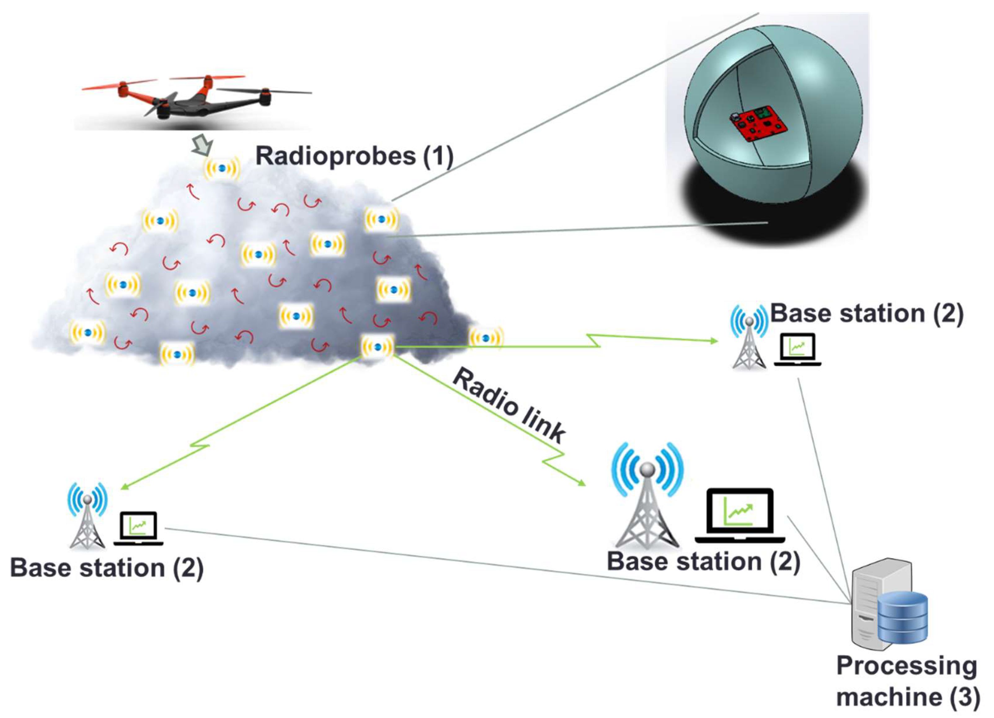
Figure 5). Unlike the previous experiment, the mini radioprobe transmitting the information was attached to a reference radiosonde, which was part of an automatic atmospheric sounding system to simulate similar conditions in which the radioprobes will be released. This experiment was carried out at the Cuneo Levaldigi meteorological station (id LIMZ) of the Regional Agency for the Protection of the Environment (ARPA) of Piedmont, Italy, where an atmospheric balloon is launched into the atmosphere twice a day. The sounding system consisted of a large helium-filled balloon of about 1.5 m in diameter, tethered by a polypropylene string a Vaisala RS41 radiosonde and able to provide temperature, humidity, wind, height, and pressure information through a telemetry link to ground stations.
The network setup for this measurement included a fully operational mini radioprobe gathering, processing, packing, and transmitting the information from the different sensors, and a ground station receiving, storing, and postprocessing the received messages. The tiny radioprobe was attached to the front side of the reference radiosonde’s cover and activated just before the launch to save energy for the flight. The radioprobe’s transceiver was programmed to provide an output power of 14 dBm at a central frequency of 865.2 MHz, spreading factor of 10, and bandwidth of 125 kHz. The receiver was placed close to the ground at an approximated height of 1 m. Because this set of measurements was carried out in a nonobstructed open environment, the transmitter was in LOS with the receiver at all positions. The system setup and trajectory followed by the systems with respect to the ground station are shown in
Figure 5 and
Figure 6, respectively.
As a result of these propagation measurements, the maximum transmission range reached by the radioprobe system in an open environment was determined. Although the reference atmospheric sounding system was intended for vertical atmospheric profiling measurements of the troposphere and low stratosphere and not for warm-cloud environments with heights between 1 and 2 km, it provided a good reference to test our system in a dynamic atmosphere environment free of obstacles. A summary of the obtained results of the measurements is reported in
Table 3.
The reference atmospheric sounding system carrying the attached mini radioprobe reached a maximum height of approximately 32 km and a horizontal range of approximately 108 km before the balloon burst. The tiny radioprobe reached a maximum height of approximately 11 km, a horizontal range of 7 km, and a straight distance of 13 km before losing contact with the ground station. In total, 462 packets were sent from the mini radioprobe during the flying time for a time span of approximately 22 min after the launch.
For all the measurements, the SNR ranged from +5 dB at the nearest distances to −1 dB at the longest ones. As expected, the RSSI of the packets decreased with the increase in distance between the transmitter and the receiver. Although there was an intermittency in the reception of some packets due to the high ascending velocity of the sounding system, the percentage of received packets for the first 5 km was higher than 90%. This is a good indicator for a warm-cloud monitoring system where the intended observation heights are between 1 and 2 km with much lower fluctuation velocities.
The communication technology was also used to demonstrate that the materials used for the bioenvelope of the radioprobe is sufficiently transparent to radio waves and does not hamper the electromagnetic transmission; that said, this study will be fully described in a future paper related to the biodegradable balloon development.
4.2. Sensors Testing and Validation
For the purpose of properly calibrating and validating the temperature and humidity sensors’ response, a set of tests were carried out in the Applied Thermodynamics Laboratory of the Italian National Metrology Institute (INRiM). A climatic chamber Kambic KK190 CHLT specifically developed for meteorology and climate metrology was used [
49]. It allows temperature regulation in the range from −40 °C to 180 °C and relative-humidity control in the range from 10% to 98% RH. The reference temperature values were obtained through four platinum resistance thermometers (Pt100) calibrated in INRiM laboratory placed inside the climatic chamber. Pt100 are read using external precision Super-Thermometer FLUKE 1594a. The reference humidity value was obtained with a Delta Ohm humidity and temperature probe calibrated at INRiM connected to a datalogger model HD27.17TS. The uncertainty of the Pt100 ranges from 0.011 °C for positive temperatures and 0.020 °C for negative temperatures. The total uncertainty of the Delta Ohm probe declared is ±3% RH.
In order to test not only the accuracy of the temperature and humidity radioprobe sensors but also to have an idea of the possible spread of their behavior, three radioprobe electronic boards were used for this experiment. They were placed inside the climatic chamber, together with reference temperature sensors and humidity probes for comparison purposes. The temperature and relative-humidity measurements from the BME280 were extracted through reading commands implemented in the microcontroller through the I2C communication interface at a sampling frequency of 1 Hz.
The climate chamber was set at temperature of +20 °C and a relative humidity of 30% RH as initial configuration. Then, additional controlled variations of chamber environment in terms of temperature and humidity were applied. In the first test, small incremental steps of 2 °C in temperature were realized (keeping RH at 30%) until reaching T = +24 °C, each one for a time span of approximately 30 min. After that the climatic chamber was configured to provide larger controlled variations in temperature starting from the current set values T = +24 °C, RH = 30% until reaching −5, 0 and 10 °C. Temperature steps need a time span of approximately 1 h each to obtain temperature stability of the whole system. This temperature cycle was done in order to simulate conditions faced by the radioprobes on site. Although warm clouds are composed only of liquid water having temperatures above 0 °C (32 °F), the cycle also included negative temperature values to test the sensors’ performance under extreme situations. The measurement results obtained in the second test are shown in
Figure 7.
In the third test, the relative humidity was changed from 10% RH to 20%, 40% and 60%, at a constant temperature of +30 °C; each step needs a time span of approximately 30 min. In order to statistically compare the obtained data, the Makima interpolation technique, which is an algorithm for one-dimensional interpolation, was used considering, at each set point, approximately 5 min of data selected when temperature and humidity conditions inside the chamber are stable. The statistical results of the second and third tests are shown in
Table 4 and
Table 5.
As a result of this experiment using a high-precision climatic chamber and calibrated reference sensors, the performance of the radioprobe sensors was evaluated. The behavior of the radioprobe sensors lies between the specifications given by the manufacturer for most of the cases (i.e., temperature accuracy ±1 °C and relative humidity ±3% RH). There are a few exceptions for the relative-humidity measurements that might be caused by the uncertainties introduced by the reference sensor itself (accuracy of the humidity reference sensor ±3% RH).
An additional field experiment was carried out to verify the response of the temperature, pressure, and humidity sensor stage nested within the radioprobe board. The data obtained came from the experiment setup using the ARPA sounding system already described in
Section 4.1: antenna matching and data transmission ranges. The fully operational mini radioprobe was fixed to the front side of the reference Vaisala RS41-SG radiosonde case with the help of a nonconductive adhesive tape. It was constantly measuring, processing, packing, and transmitting the information to the base station located on the ground. The reference probe incorporated a temperature sensor using a linear resistive platinum technology, a humidity sensor integrating humidity, and additional temperature sensing elements, and a GPS receiver allowing the derivation of pressure, height, and wind data [
50]. Regarding the accuracy provided by the reference instrument, the uncertainties declared for sounding are 0.3 °C for temperature measurements (below 16 km), 4% RH for humidity measurements, and 1.0 hPa/0.5 hPa for pressure measurements (for pressure values greater that 100 hPa). In order to statistically compare the obtained data, the set of measurements considered for the analysis corresponds to the interval up to which the percentage of received packets was greater than 90%. At this point, the straight distance between the flying system and the base station was approximately 5 km. The measurement results obtained are shown in
Figure 8. The statistical results of this test are shown in
Table 6.
As a result of this experiment using a VAISALA radiosonde as a reference, the performance of the radioprobe’s temperature, humidity, and pressure sensor block was evaluated. From
Figure 8, it is possible to observe some differences between the measurements provided by the radioprobe sensors and the reference instrument. These effects could have been produced by the position itself of the mini radioprobe onto the case containing the reference probe. Due to the lack of space available for placing the radioprobe and for avoiding its fall during the flight, it was tightly attached to the reference probe leading to potential undesired effects. For instance, being in direct contact with the main body of reference instrument case, the energy dissipated by the reference probe could have affected the radioprobe measurements. Also, since the airflow in direction to the vent hole of the TPH sensors was partially obstructed, the exchange of sufficient air was not possible, contributing to errors in the measurements. Notwithstanding the aforementioned issues and considering the limited resources in the design (e.g., small size, ultralight weight, low-power and low-cost sensors), it can be said from the obtained results that the performance of the TPH radioprobe sensors is good enough for the purpose of the radioprobe development. Overall, considering the uncertainties introduced by the reference sensors, the behavior of the TPH radioprobe sensors lies within the specifications given by the manufacturer, as can be seen in
Table 6.
Future experiments will include a different setup of the instruments to overcome the problems encountered during the execution of this field experiment.
To validate the radioprobe’s positioning and tracking system, it was compared to GPS data from a smartphone device. This test was carried out in an open area within the city of Turin. The system setup included a radioprobe measuring and partially processing the readings from the IMU sensors (accelerometer, gyroscope, and magnetometer), and gathering the geolocation and time updates from the GNSS receiver. The radioprobe was configured in order to provide a GNSS sensor update every 2 s and two IMU sensor updates every second. It was connected via serial port to a portable PC for data logging. Additionally, an Android-based smartphone model Samsung Galaxy S8+ executing a GNSS logger application for recording the position and path followed was used. This application provided positioning updates for every second.
For this experiment, the radioprobe and the smartphone simultaneously recorded data during a walk. Before starting the measurements, the calibration of the IMU sensors was performed to ensure that the readings and the output of the prefiltering process executed at the radioprobe side were accurate. While being at rest, the bias errors and noise introduced by the accelerometer, gyroscope, and magnetometer were properly identified. In addition, since the GNSS update frequencies between the reference and radioprobe were different, the IMU readings were used to predict positioning information for the intermediate time steps. To this end, the IMU sensor data were processed using Madgwick filtering, which is an orientation algorithm to describe orientation in three-dimensions [
51], to get accelerations in NED (north, east, and down) absolute frame. This frame is useful for the postprocessing analysis to predict the radioprobe’s position along its trajectory. Thus, acceleration data in absolute frame can be combined with LLA (latitude, longitude, and altitude) absolute positioning data coming from the GNSS server. In this way, it is possible to have five (one GNSS update and four predictions with IMU data) positioning information for every 2 s. The raw acceleration data along x, y, and z directions in the radioprobe’s body frame and the converted acceleration in absolute frame after applying the orientation filter are shown in
Figure 9. Since the experiment was performed in a horizontal plane, it is possible to see the north and east accelerations around zero, except for small fluctuations due to walk maneuver. Instead, for the down direction, the acceleration was around 10 m/s
2 because of gravity.
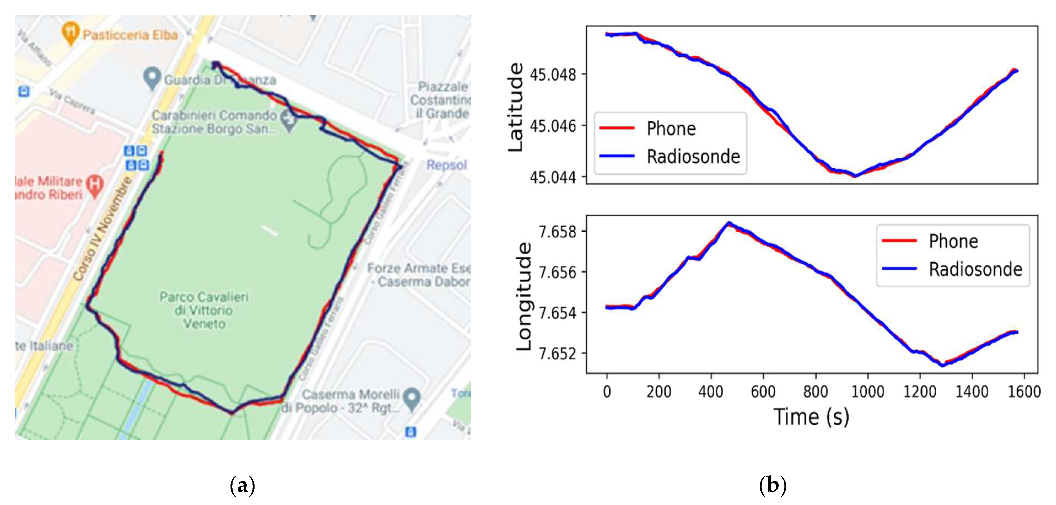
During the experiment, the total traveled distance from the starting to the final points was approximately 1.6 km for a time span of approximately 30 min. The trajectory recorded by both systems together with the comparison between trajectories along north (Latitude) and east (longitude) directions are shown in
Figure 10. The statistical results of the positioning sensors accuracy (IMU and GNSS) are shown in
Table 7.
From the obtained results, it is possible to verify the reasonable performance of the positioning and tracking radioprobe sensor unit considering the limited resources at the radioprobe side (e.g., low power, low memory availability, light weight and not-expensive sensors). To overcome these challenges, the reduction of the IMU sampling rate and the activation of a GNSS super-saving mode (E-mode) are among the strategies used. The partially processed data generated at this stage constitute the input for the further postprocessing step executed at the ground level to reconstruct the trajectory followed by the mini radioprobes.
An additional experiment to validate the positioning and tracking radioprobe sensor unit was conducted. Although the balloon’s performance analysis is not the purpose of this work, we carried out a preliminary tethered-balloon test at low altitude (30–50 m) to expose the radioprobe to real atmospheric air fluctuation and verify the fluctuation detection ability of the tiny radioprobe when flying. This test was carried out at Parco Piemonte, which is a wide tree-free park located at the south area of Turin. The field measurement consisted of a point-to-point dynamic network configuration including a fully operational radioprobe collecting and transmitting the about-flight information, and a ground station receiving, storing, and postprocessing the received messages. The mini radioprobe was inserted in the middle of the helium-filled biodegradable balloon and released into the low atmosphere. In order to not lose the measuring system, the balloon was attached to a long thin thread and held by one of the participants. The radioprobe’s transceiver was programmed to provide an output power of 14 dBm at a central frequency of 865.2 MHz, spreading factor of 10, and bandwidth of 125 kHz. The receiver was placed close to the ground at an approximated height of 1 m and at an approximate distance of 25 m from the initial balloon release point. Both the transmitter and the receiver were in LOS during the execution of the experiment. The trajectory followed by the radioprobe during the flight is shown in
Figure 11.
The IMU measurements (acceleration, angular rate, and magnetic field) are displayed in
Figure 12.
As a result of this experiment, the fully operational radioprobe was tested in a low-atmosphere open environment. The obtained results show the good radioprobe capacity to detect acceleration, angular rate, and magnetic-field fluctuations while flying inside the balloon in a dynamic environment. In addition, all the transmitted packets sent by the moving instrument were correctly received at the ground station. The SNR values ranged from +9 to −12 dB and the RSSI of the packets from −65 to −109 dBm.


 ,
, 


