Sequential Sampling and Estimation of Approximately Bandlimited Graph Signals

Abstract

Graph signal sampling has been widely studied in recent years, but the accurate signal models required by most of the existing sampling methods are usually unavailable prior to any observations made in a practical environment. In this paper, a sequential sampling and estimation algorithm is proposed for approximately bandlimited graph signals, in the absence of prior knowledge concerning signal properties. We approach the problem from a Bayesian perspective in which we formulate the signal prior by a multivariate Gaussian distribution with unknown hyperparameters. To overcome the interconnected problems associated with the parameter estimation, in the proposed algorithm, hyperparameter estimation and sample selection are performed in an alternating way. At each step, the unknown hyperparameters are updated by an expectation maximization procedure based on historical observations, and then the next node in the sampling operation is chosen by uncertainty sampling with the latest hyperparameters. We prove that under some specific conditions, signal estimation in the proposed algorithm is consistent. Subsequent validation of the approach through simulations shows that the proposed procedure yields performances which are significantly better than existing state-of-the-art approaches notwithstanding the additional attribute of robustness in the presence of a broad range of signal attributes.

1. Introduction

Graph signal is a powerful tool to represent and analyze data with irregular interconnections by defining signal values on graph vertices and assigning edge weights according to correlation or similarity [1]. In the past decade, graph signal processing theory has developed rapidly, extending classical signal processing techniques such as Fourier analysis [1,2], filtering [3,4,5], sampling and interpolation [6,7,8] to graph signal setting. Related concepts and methods have found wide application in sensor networks [9,10], brain analysis [11], image processing [12], three-dimensional (3D) point cloud processing [13], and machine learning [14,15,16].

Sampling for (lossless) reconstruction or (minimum error) estimation is a fundamental problem in graph signal processing. For example, a sample survey in a social network needs to carefully select interviewees so as to better predict the attitudes of all users. In a sensor network, it is important to optimize sensor placement so that more information can be collected by a restricted number of sensors due to economic constraint [9]. In addition, any graph-based active semisupervised learning task may also be interpreted as a graph signal sampling and estimation problem [14,15].

There have been multiple works on graph signal sampling. The authors of [6,7] try to extend the Nyquist sampling theory to bandlimited graph signals. More works are seeking optimal sampling sets for graph signal estimation, where the graph signals are usually assumed to be bandlimited [17,18,19] or approximately bandlimited [17,20] in the frequency domain, or smooth in the vertex domain [17,21]. Sampling strategies mainly include topology-based methods that compute a score for each vertex [18,21], and design-of-experiment (DOE) approaches that optimize certain scalarization form of some target matrix [19,22]. Most of the current sampling methods rely on accurate bandwidth [6,18,19] or prior distribution [22,23] of the graph signal.

It is natural in many applications to assume that the graph signal is somehow bandlimited or smooth. For instance, people with strong social connection are likely to hold similar opinions and temperature sensors located close to each other usually get similar measurements. However, in practice it is hard to know the exact bandwidth or prior distribution of the graph signal before any observation. In such cases, those sampling strategies based on accurate signal model become not applicable.

A possible solution is to sample and estimate in a sequential way. Unknown signal properties can be estimated from previous observations, and the subsequent sampling node can be selected under the latest signal model. Such a sequential framework can overcome the difficulty of incomplete system model and take advantage of model-based sample selection and signal estimation [20].

In this work, we investigate the sequential sampling and estimation of approximately bandlimited (ABL) graph signals, whose bandwidth and energy level are both not known in advance. With the aid of a Butterworth low-pass filter, the ABL graph signal is assumed to follow a multivariate Gaussian distribution with unknown hyperparameters. The variance of observation noise is also considered unknown.

In the proposed algorithm, hyperparameter estimation and sample selection are performed in an alternating way. At each step, expectation maximization (EM) [24] is first used to update the maximum marginal likelihood (MML) estimation of unknown hyperparameters based on historical observations. Substituting these latest estimated values into the signal prior and noise distribution, a Bayesian estimation and prediction procedure can then be performed. According to the uncertainty sampling (US) criterion [25], the node with the largest predictive variance is selected as the next node to sample.

In fact, estimating prior distribution from data, namely, empirical Bayes (EB) method, has long been studied [26]. It has been proved that under certain assumptions, the EB posterior distribution of parameter is consistent at its true value [27]. Meanwhile, an alternating approach analogous to the proposed one has been used in sequential DOE for nonlinear least squares (LS) regression. There, parameter estimation is proved to be consistent, and the design is asymptotically optimal [28].

In this paper, we prove that under specific conditions, signal estimation in the proposed algorithm is consistent at the true value. That is, as the number of samples goes to infinity, the estimated graph signal can get arbitrarily close to the true value. The finite-time performance of the proposed algorithm is validated by simulation results. Our algorithm is able to adjust to ABL graph signals with different properties, and it performs better in estimation error than existing methods.

The rest of the paper is organized as follows. We detail the signal prior and observation model in Section 2, and develop a sequential sampling and estimation algorithm in Section 3. The consistency of the proposed algorithm is proved under specific conditions in Section 4, and its finite-time performance is validated by experiments in Section 5. We conclude the paper in Section 6.

Throughout the paper, we use normal-weight italic lowercase letters (e.g., x) to denote scalar variables, bold italic lowercase letters (e.g., $\mathit{x}$) to denote vectors, bold italic uppercase letters (e.g., $\mathit{X}$) to denote matrices, and calligraphic uppercase letters (e.g., $\mathcal{X}$) to denote sets.

2. System Model

2.1. Preliminaries

We consider a simple connected weighted undirected graph $\mathcal{G}=(\mathcal{V},\mathcal{E},\mathit{W})$, where $\mathcal{V}$ is the set of vertices indexed by $\{1,\dots ,N\}$; $\mathcal{E}$ is the set of edges between vertex pairs, e.g., $(i,j)\in \mathcal{E}$ denotes an edge between vertex i and vertex j; and $\mathit{W}$ is the weighted adjacency matrix, with $w_{ij}$ the weight of edge between vertex i and vertex j if they are connected, or 0 otherwise. A graph signal that takes a real value on each vertex of the graph can be represented as $\mathit{f}\in {\mathbb{R}}^N$, where $f_i$ is the signal value on vertex i.

The Laplacian matrix is defined as $\mathit{L}=\mathit{D}-\mathit{W}$, where $\mathit{D}=\dots (d_1,\dots ,d_N)$ with $d_i={\sum }_{j:(i,j)\in \mathcal{E}}{w}_{ij}$ is the degree matrix. Being symmetric and positive semi-definite, $\mathit{L}$ has a spectral decomposition $\mathit{L}=\mathit{V}\mathsf{\Lambda }{\mathit{V}}^T$, where $\mathsf{\Lambda }$ is a diagonal matrix of the eigenvalues $0={\lambda }_1<{\lambda }_2\le \cdots \le {\lambda }_N$, and $\mathit{V}$ contains the corresponding orthonormal eigenvectors ${\left\{{\mathit{v}}_k\right\}}_{k=1}^N$ as columns. These eigenvectors act as graph Fourier basis, and the associated eigenvalues are regarded as graph frequencies [1]. The frequency-domain coefficients $\widehat{\mathit{f}}$ of a graph signal $\mathit{f}$ can be calculated via the graph Fourier transform (GFT) as $\widehat{\mathit{f}}={\mathit{V}}^T\mathit{f}$. The graph signal $\mathit{f}$ can be expressed as $\mathit{f}=\mathit{V}\widehat{\mathit{f}}$, which is known as the inverse GFT (IGFT).

2.2. Signal Prior

In this work, the graph signal $\mathit{f}$ is assumed to be drawn from the following distribution:

$$p(\mathit{f};\alpha ,\gamma )=\mathcal{N}\left(\mathit{f}\right|\mathit{0},{(\alpha {\mathit{I}}_N+\gamma {\mathit{L}}^{2n})}^{-1}),$$

(1)

where ${\mathit{I}}_N$ denotes the $N\times N$ identity matrix, and $n,\alpha ,\gamma >0$ are hyperparameters, among which $\alpha ,\gamma$ are assumed unknown in prior. The meanings of the signal model and hyperparameters are explained in the frequency domain as follows.

By GFT, the spectral coefficients ${\left\{{\widehat{f}}_k\right\}}_{k=1}^N$ follow independent zero-mean Gaussian distributions with variances conforming to a Butterworth low-pass filter ([29], Section 7.3):

$$p\left({\widehat{f}}_k\right)=\mathcal{N}\left({\widehat{f}}_k|0,{\displaystyle \frac{g^2}{1+{({\lambda }_k/{\lambda }_{\mathrm{c}})}^{2n}}}\right),$$

(2)

where n is the order, ${\lambda }_{\mathrm{c}}=\sqrt[2n]{\alpha /\gamma }$ is the cut-off frequency, and $g=1/\sqrt{\alpha }$ is the amplitude gain of the filter. Under such a prior, we say the graph signal is approximately bandlimited in a probabilistic sense, where ${\lambda }_{\mathrm{c}}$ plays the role of bandwidth, n controls the strictness of banlimitedness, and g determines the energy level of the graph signal.

Specially, when $n=1/2$ and $\delta =\alpha /\gamma$ is small, the signal prior Equation (1) becomes

$$p\left(\mathit{f}\right)\propto exp\left(-{\displaystyle \frac{\gamma }{2}}{\mathit{f}}^T(\mathit{L}+\delta {\mathit{I}}_N)\mathit{f}\right),$$

(3)

which is widely used in graph signal sampling and estimation [9,23]. The restriction on total variation ${\mathit{f}}^T\mathit{L}\mathit{f}={\sum }_{(i,j)\in \mathcal{E}}{w}_{ij}{(f_i-f_j)}^2$ can lead to smooth signals over the graph.

If $n\to \infty$, the out-of-band coefficients become deterministic zeros. The graph signal becomes strictly bandlimited, represented by

$$\mathit{f}={\mathit{V}}_K{\widehat{\mathit{f}}}_K,$$

(4)

where $K=max\left\{k\right|{\lambda }_k\le {\lambda }_{\mathrm{c}}\}$, ${\widehat{\mathit{f}}}_K$ collects the first K GFT coefficients that may be non-zero, and ${\mathit{V}}_K$ contains the first K GFT basis.

In conclusion, our signal prior Equation (1) is flexible to describe approximately bandlimited graph signals with different bandwidth, strictness of bandlimitedness, and energy level. It can also cover the most commonly used smoothness prior [9,23] and bandlimitedness prior [6,7,18,19]. Additionally, this model is simple with three hyperparameters, and can be represented in the vertex domain without eigendecomposition.

Here, hyperparameters $\alpha ,\gamma$ or equivalently ${\lambda }_{\mathrm{c}},g$ in the signal prior are assumed unknown, that is, we do not need to have prior knowledge about the bandwidth or energy level of the graph signal. Only a value for n is required to control the strictness of bandlimitedness of the estimated signal. Compared to those methods for only strictly bandlimited graph signals with known bandwidth or smooth graph signals with known prior distribution, our signal prior is more general.

2.3. Observation Model

To overcome the difficulty caused by unknown hyperparameters, a sequential sampling process is considered, where one node is sampled at each step, so that unknown hyperparameters can be estimated from previous observations, and the next node to sample can be selected using the latest hyperparameters.

Suppose that vertex $s_t$ is sampled at step t, and the observed signal value is $y_t$. The observation model can be expressed as

$$y_t={\mathit{\psi }}_t^T\mathit{f}+w_t,$$

(5)

where ${\mathit{\psi }}_t^T={\mathit{e}}_{s_t}^T$ is the sampling vector with its $s_t$-th element equal to 1 and others equal to 0, and $w_t$ is an additive zero-mean Gaussian observation noise with unknown precision $\beta$,

$$p(w_t;\beta )=\mathcal{N}\left(w_t\right|0,{\beta }^{-1}).$$

(6)

In hyperparameter, signal estimation, and sample selection at step t, the historical observations from step 1 to step t are considered together. Let

$${\mathit{y}}_{1:t}=\left[\begin{array}{c}{y}_1\\ ⋮\\ y_t\end{array}\right],{\mathsf{\Psi }}_{1:t}=\left[\begin{array}{c}{\mathit{\psi }}_1^T\\ ⋮\\ {\mathit{\psi }}_t^T\end{array}\right]=\left[\begin{array}{c}{\mathit{e}}_{s_1}^T\\ ⋮\\ {\mathit{e}}_{s_t}^T\end{array}\right],{\mathit{w}}_{1:t}=\left[\begin{array}{c}{w}_1\\ ⋮\\ w_t\end{array}\right].$$

(7)

The noise values $w_1,\dots ,w_t$ involved in different samples (on either different vertices or the same vertex) are assumed to be independent and identically distributed (i.i.d.). According to Equations (5) and (6),

$$\begin{array}{c}{\mathit{y}}_{1:t}={\mathsf{\Psi }}_{1:t}\mathit{f}+{\mathit{w}}_{1:t},\end{array}$$

(8)

$$\begin{array}{c}p({\mathit{w}}_{1:t};\beta )=\mathcal{N}\left({\mathit{w}}_{1:t}\right|\mathit{0},{\beta }^{-1}{\mathit{I}}_t).\end{array}$$

(9)

2.4. Problem Formulation

Under the signal and observation model described in Section 2.2 and Section 2.3, at each step t in the sequential sampling and estimation process, the two core problems are (1) how to estimate the unknown hyperparameters $\alpha ,\gamma ,\beta$ as well as the graph signal $\mathit{f}$ based on the historical observations ${\mathsf{\Psi }}_{1:t},{\mathit{y}}_{1:t}$

$${\alpha }_t^{\prime },{\gamma }_t^{\prime },{\beta }_t^{\prime },{\mathit{f}}_t^{\prime }↤{\mathsf{\Psi }}_{1:t},{\mathit{y}}_{1:t},$$

(10)

where ${\alpha }_t^{\prime },{\gamma }_t^{\prime },{\beta }_t^{\prime }$ are the estimated values of hyperparameters at step t, and ${\mathit{f}}_t^{\prime }$ denotes the estimated graph signal at step t, and (2) how to select the next node $s_{t+1}$ to be sampled at step $t+1$ with the latest estimated values of hyperparameters

$$s_{t+1}↤{\mathsf{\Psi }}_{1:t},{\mathit{y}}_{1:t},{\alpha }_t^{\prime },{\gamma }_t^{\prime },{\beta }_t^{\prime }.$$

(11)

Our ultimate goal is to minimize signal estimation error within given budget, or from another angle, reach certain estimation accuracy with least samples.

3. Algorithm

3.1. Hyperparameter and Signal Estimation

We first focus on unknown hyperparameter estimation from observation data. Here, maximum marginal likelihood (MML) estimation of unknown hyperparameters is adopted:

$$\begin{array}{cc}\hfill {\alpha }_t^{\prime },{\gamma }_t^{\prime },{\beta }_t^{\prime }& =arg\underset{\alpha ,\gamma ,\beta }{max}p\left({\mathit{y}}_{1:t}\right|{\mathsf{\Psi }}_{1:t};\alpha ,\gamma ,\beta )\hfill \\ \hfill & =arg\underset{\alpha ,\gamma ,\beta }{max}{\int }_{{\mathbb{R}}^N}p\left({\mathit{y}}_{1:t}\right|{\mathsf{\Psi }}_{1:t},\mathit{f};\beta )p(\mathit{f};\alpha ,\gamma )d\mathit{f}.\hfill \end{array}$$

(12)

Then, the signal posterior given estimated hyperparameters is Gaussian:

$$p\left(\mathit{f}\right|{\mathsf{\Psi }}_{1:t},{\mathit{y}}_{1:t};{\alpha }_t^{\prime },{\gamma }_t^{\prime },{\beta }_t^{\prime })=\mathcal{N}\left(\mathit{f}\right|{\mathit{\mu }}_t,{\mathit{C}}_t),$$

(13)

with mean vector and covariance matrix ([30], Section 10.6)

$$\begin{array}{cc}\hfill & {\mathit{\mu }}_t={\beta }_t^{\prime }{\mathit{C}}_t{\mathsf{\Psi }}_{1:t}^T{\mathit{y}}_{1:t},\hfill \end{array}$$

(14)

$$\begin{array}{cc}\hfill & {\mathit{C}}_t={({\alpha }_t^{\prime }{\mathit{I}}_N+{\gamma }_t^{\prime }{\mathit{L}}^{2n}+{\beta }_t^{\prime }{\mathsf{\Psi }}_{1:t}^T{\mathsf{\Psi }}_{1:t})}^{-1}.\hfill \end{array}$$

(15)

The minimum mean square error (MMSE) or maximum a posteriori (MAP) estimation of the graph signal is ${\mathit{f}}_t^{\prime }={\mathit{\mu }}_t$.

However, direct optimization of Equation (12) is intractable. We view $\mathit{f}$ as a hidden variable, and introduce expectation maximization (EM) ([24], Section 9.4) in our algorithm to estimate $\alpha ,\gamma ,\beta$, and thereby obtain the posterior distribution of $\mathit{f}$. To be concise, the subscripts t and $1:t$ are omitted in the introduction of our EM algorithm.

Consider the l-th EM iteration. In E step, hyperparameters $\alpha ,\gamma ,\beta$ are fixed at ${\alpha }_{l-1},{\gamma }_{l-1},$ ${\beta }_{l-1}$, and the signal posterior $p\left(\mathit{f}\right|\mathsf{\Psi },\mathit{y};{\alpha }_{l-1},{\gamma }_{l-1},{\beta }_{l-1})$ with mean ${\mathit{\mu }}_{l-1}$ and covariance ${\mathit{C}}_{l-1}$ is computed as in Equations (13)–(15).

In M step, $\alpha ,\gamma ,\beta$ are updated according to

$$\begin{array}{cc}\hfill {\alpha }_l,{\gamma }_l,{\beta }_l& =arg\underset{\alpha ,\gamma ,\beta }{max}{\mathbb{E}}_{\mathit{f}|\mathsf{\Psi },\mathit{y};{\alpha }_{l-1},{\gamma }_{l-1},{\beta }_{l-1}}[lnp(\mathit{y},\mathit{f}|\mathsf{\Psi };\alpha ,\gamma ,\beta )]\hfill \\ \hfill & =arg\underset{\alpha ,\gamma ,\beta }{max}{\mathbb{E}}_{\mathit{f}|\mathsf{\Psi },\mathit{y};{\alpha }_{l-1},{\gamma }_{l-1},{\beta }_{l-1}}[lnp\left(\mathit{y}\right|\mathsf{\Psi },\mathit{f};\beta )+lnp(\mathit{f};\alpha ,\gamma )],\hfill \end{array}$$

(16)

where ${\mathbb{E}}_{\mathit{f}|\mathsf{\Psi },\mathit{y};{\alpha }_{l-1},{\gamma }_{l-1},{\beta }_{l-1}}[·]$ means the expectation is taken with respect to $p\left(\mathit{f}\right|\mathsf{\Psi },\mathit{y};{\alpha }_{l-1},$ ${\gamma }_{l-1},{\beta }_{l-1})$ computed at E step, the signal prior $p(\mathit{f};\alpha ,\gamma )$ is given in Equation (1), and the signal likelihood $p\left(\mathit{y}\right|\mathsf{\Psi },\mathit{f};\beta )=\mathcal{N}\left(\mathit{y}\right|\mathsf{\Psi }\mathit{f},{\beta }^{-1}\mathit{I})$ according to Equations (8) and (9).

For brevity, denote the expectation operator in Equation (16) as ${\mathbb{E}}_{l-1}[·]$, and the expectation value as $E_{l-1}$, which is also the objective value of the optimization problem. By direct calculations, we have

$$\begin{array}{cc}\hfill E_{l-1}=& {\displaystyle \frac{1}{2}}ln|\alpha {\mathit{I}}_N+\gamma {\mathit{L}}^{2n}|-{\displaystyle \frac{\alpha }{2}}{\mathbb{E}}_{l-1}\left[{\mathit{f}}^T\mathit{f}\right]-{\displaystyle \frac{\gamma }{2}}{\mathbb{E}}_{l-1}\left[{\mathit{f}}^T{\mathit{L}}^{2n}\mathit{f}\right]\hfill \\ \hfill & +{\displaystyle \frac{M}{2}}ln\beta -{\displaystyle \frac{\beta }{2}}{\mathbb{E}}_{l-1}\left[{(\mathit{y}-\mathsf{\Psi }\mathit{f})}^T(\mathit{y}-\mathsf{\Psi }\mathit{f})\right]+\mathrm{const},\hfill \end{array}$$

(17)

where M is the sample size; “const” denotes terms that are independent of $\alpha ,\gamma ,\beta$; and

$$\begin{array}{cc}{\mathbb{E}}_{l-1}\left[{\mathit{f}}^T\mathit{f}\right]\hfill & ={\mathbb{E}}_{l-1}[{(\mathit{f}-{\mathit{\mu }}_{l-1})}^T(\mathit{f}-{\mathit{\mu }}_{l-1})+2{\mathit{\mu }}_{l-1}^T\mathit{f}-{\mathit{\mu }}_{l-1}^T{\mathit{\mu }}_{l-1}]\hfill \\ \hfill & =\dots \left({\mathit{C}}_{l-1}\right)+{\mathit{\mu }}_{l-1}^T{\mathit{\mu }}_{l-1},\hfill \end{array}$$

(18)

$$\begin{array}{cc}{\mathbb{E}}_{l-1}\left[{\mathit{f}}^T{\mathit{L}}^{2n}\mathit{f}\right]\hfill & ={\mathbb{E}}_{l-1}[{(\mathit{f}-{\mathit{\mu }}_{l-1})}^T{\mathit{L}}^{2n}(\mathit{f}-{\mathit{\mu }}_{l-1})+2{\mathit{\mu }}_{l-1}^T{\mathit{L}}^{2n}\mathit{f}-{\mathit{\mu }}_{l-1}^T{\mathit{L}}^{2n}{\mathit{\mu }}_{l-1}]\hfill \\ \hfill & =\dots \left({\mathit{L}}^{2n}{\mathit{C}}_{l-1}\right)+{\mathit{\mu }}_{l-1}^T{\mathit{L}}^{2n}{\mathit{\mu }}_{l-1},\hfill \end{array}$$

(19)

$$\begin{array}{cc}{\mathbb{E}}_{l-1}\left[{(\mathit{y}-\mathsf{\Psi }\mathit{f})}^T(\mathit{y}-\mathsf{\Psi }\mathit{f})\right]\hfill & ={\mathbb{E}}_{l-1}[{(\mathit{y}-\mathsf{\Psi }{\mathit{\mu }}_{l-1})}^T(\mathit{y}-\mathsf{\Psi }{\mathit{\mu }}_{l-1})\hfill \\ \hfill & -2{(\mathit{y}-\mathsf{\Psi }{\mathit{\mu }}_{l-1})}^T\mathsf{\Psi }(\mathit{f}-{\mathit{\mu }}_{l-1})\hfill \\ \hfill & +{(\mathit{f}-{\mathit{\mu }}_{l-1})}^T{\mathsf{\Psi }}^T\mathsf{\Psi }(\mathit{f}-{\mathit{\mu }}_{l-1})]\hfill \\ \hfill & ={(\mathit{y}-\mathsf{\Psi }{\mathit{\mu }}_{l-1})}^T(\mathit{y}-\mathsf{\Psi }{\mathit{\mu }}_{l-1})+\dots \left({\mathsf{\Psi }}^T\mathsf{\Psi }{\mathit{C}}_{l-1}\right).\hfill \end{array}$$

(20)

Note that $E_{l-1}$ is concave with respect to $\alpha ,\gamma ,\beta$, see Appendix A. The maximization problem in Equation (16) can be solved by any standard tool for convex optimization. Here, the first order conditions of the optimization problem are analyzed to give some insights into the hyperparameter estimation, and then a possible efficient search method based on these conditions is provided in Appendix B.

Take the partial derivatives of $E_{l-1}$ with respect to $\alpha ,\gamma ,\beta$, and set them to zero:

$$\begin{array}{cc}\hfill & {\displaystyle \frac{\partial E_{l-1}}{\partial \alpha }}={\displaystyle \frac{1}{2}}\dots \left({(\alpha {\mathit{I}}_N+\gamma {\mathit{L}}^{2n})}^{-1}\right)-{\displaystyle \frac{1}{2}}{\mathbb{E}}_{l-1}\left[{\mathit{f}}^T\mathit{f}\right]=0,\hfill \end{array}$$

(21)

$$\begin{array}{cc}\hfill & {\displaystyle \frac{\partial E_{l-1}}{\partial \gamma }}={\displaystyle \frac{1}{2}}\dots \left({(\alpha {\mathit{I}}_N+\gamma {\mathit{L}}^{2n})}^{-1}{\mathit{L}}^{2n}\right)-{\displaystyle \frac{1}{2}}{\mathbb{E}}_{l-1}\left[{\mathit{f}}^T{\mathit{L}}^{2n}\mathit{f}\right]=0,\hfill \end{array}$$

(22)

$$\begin{array}{cc}\hfill & {\displaystyle \frac{\partial E_{l-1}}{\partial \beta }}={\displaystyle \frac{M}{2\beta }}-{\displaystyle \frac{1}{2}}{\mathbb{E}}_{l-1}\left[{(\mathit{y}-\mathsf{\Psi }\mathit{f})}^T(\mathit{y}-\mathsf{\Psi }\mathit{f})\right]=0.\hfill \end{array}$$

(23)

Note that $\mathrm{tr}\left({(\alpha {\mathit{I}}_N+\gamma {\mathit{L}}^{2n})}^{-1}\right)$, $\mathrm{tr}\left({(\alpha {\mathit{I}}_N+\gamma {\mathit{L}}^{2n})}^{-1}{\mathit{L}}^{2n}\right)$ and $\frac{M}{\beta }$ can be seen as the prior expectations of ${\mathit{f}}^T\mathit{f}$, ${\mathit{f}}^T{\mathit{L}}^{2n}\mathit{f}$ and ${\mathit{w}}^T\mathit{w}$ with respect to $p(\mathit{f};\alpha ,\gamma )$ and $p(\mathit{w};\beta )$. The M step actually looks for a group of hyperparameters that makes these prior expectations equal to their posterior ones. In this sense, the estimated hyperparameters agree with the observations.

Repeat the E and M steps as above until convergence, and we will obtain an MML estimation of unknown hyperparameters $\alpha ,\gamma ,\beta$, together with a posterior of the graph signal $\mathit{f}$. This process is summarized in Algorithm 1. Although the estimated hyperparameters are not guaranteed to be globally optimal by MML, we find the performance good enough in experiments.

Algorithm 1 Hyperparameter and signal estimation by EM.

1: Initialize ${\alpha }_0,{\gamma }_0,{\beta }_0$. 2: for$l=1,2,\cdots$do 3:  Compute ${\mathit{\mu }}_{l-1},{\mathit{C}}_{l-1}$ as in Equations (14) and (15). 4:  Update ${\alpha }_l,{\gamma }_l,{\beta }_l$ according to Equation (16). 5: end for

3.2. Sample Selection

Having been able to estimate the unknown hyperparameters from previous observations by EM, at each decision step, the subsequent sampling node can be selected using the latest estimated values of hyperparameters.

According to the uncertainty sampling (US) criterion in active learning ([25], Chapter 2), we should scan through all the nodes, and pick the one whose observed signal value we are most uncertain about as the next node to sample. Here, predictive variance is regarded as a measurement of uncertainty.

The predictive distribution of an observation y on vertex s with sampling vector ${\mathit{\psi }}^T={\mathit{e}}_s^T$ given historical observations ${\mathsf{\Psi }}_{1:t},{\mathit{y}}_{1:t}$ is

$$p\left(y\right|{\mathsf{\Psi }}_{1:t},{\mathit{y}}_{1:t},{\mathit{\psi }}^T;{\alpha }_t^{\prime },{\gamma }_t^{\prime },{\beta }_t^{\prime })=\mathcal{N}\left(y\right|{\mathit{e}}_s^T{\mathit{\mu }}_t,{\mathit{e}}_s^T{\mathit{C}}_t{\mathit{e}}_s+{\left({\beta }_t^{\prime }\right)}^{-1}),$$

(24)

where ${\mathit{\mu }}_t$ and ${\mathit{C}}_t$ are the posterior mean and covariance of the graph signal $\mathit{f}$, respectively, given ${\mathsf{\Psi }}_{1:t}$ and ${\mathit{y}}_{1:t}$. The predictive variance consists of two parts: estimative variance ${\mathit{e}}_s^T{\mathit{C}}_t{\mathit{e}}_s$ and noise variance ${\left({\beta }_t^{\prime }\right)}^{-1}$, among which the latter is equal for all vertices. The next sampling node $s_{t+1}$ can be decided by

$$s_{t+1}=arg\underset{s\in \mathcal{V}}{max}{\mathit{e}}_s^T{\mathit{C}}_t{\mathit{e}}_s.$$

(25)

3.3. Sequential Sampling and Estimation

Finally, the complete procedure of the proposed sequential sampling and estimation algorithm for approximately bandlimited graph signals is given in Algorithm 2. At each step, first unknown hyperparameters are re-estimated by EM as in Section 3.1, and then the next node to sample is selected by US as in Section 3.2. The total number of sampling steps T is equal to the sampling budget.

Algorithm 2 Sequential sampling and estimation of approximately bandlimited graph signals.

1: Choose the first sampling node $s_1$ arbitrarily. 2: for$t=1,2,\dots$do 3:  Sample the vertex $s_t$ and obtain an observation $y_t$. 4:  Update hyperparameters ${\alpha }_t^{\prime },{\gamma }_t^{\prime },{\beta }_t^{\prime }$ and signal posterior ${\mathit{\mu }}_t,{\mathit{C}}_t$ by EM as in Algorithm 1. 5:  Select the next node to sample $s_{t+1}$ by US as in Equation (25). 6: end for

Our sequential sampling strategy takes into account not only graph topology, but also previous observations, by both estimating hyperparameters based on historical data and selecting sampling nodes based on signal posterior. Making full use of historical observations and deciding which nodes to sample online, the proposed algorithm is able to cope with the situation where signal and noise distributions are not completely available in advance, and efficiently select samples to estimate the underlying graph signal.

The computational complexity of a decision step in the proposed algorithm is $O\left(n_t^{\mathrm{EM}}\overline{n_t^{\mathrm{bs}}}{N}^3\right)$, where $n_t^{\mathrm{EM}}$ is the number of EM iterations, $\overline{n_t^{\mathrm{bs}}}$ is the average iterations of binary search in M step, and N is the graph size. The computational cost is acceptable in view of the performance improvement, especially in time-insensitive scenarios with large observation cost. The proposed method is able to efficiently select samples to give accurate estimation of signals thanks to the sequential framework with EM hyperparameter update, and the signal estimation is consistent.

4. Asymptotic Analysis

In the previous section, we have developed a sequential sampling and estimation algorithm for approximately bandlimited graph signals with an incomplete system model, where hyperparameter estimation and sample selection are performed in an alternating way. The performance of the proposed algorithm will be validated via simulation in the next section, where we will see its efficient sample selection and accurate signal estimation with limited sampling budget and little prior knowledge. In this section, we are to emphasize that the proposed algorithm improves limited-budget performance without sacrifice of consistency, which is not trivial for a sequential decision process.

Intuitively, as the number of observations grows, hyperparameters better fitting the true model will be picked out, really important nodes will be selected to sample, and finally an excellent estimation of the graph signal can be obtained. Here, we try to provide some theoretical support for this intuition. The asymptotic performance of the proposed algorithm is analyzed, and we state and prove the consistency of signal estimation in our method.

Before concentrating on the asymptotic performance of signal estimation, we first investigate the asymptotic behavior of sample selection in the proposed algorithm.

Lemma 1.

Let $m_{i,t}$ denote the number of times vertex i is sampled up to step t. If $\underset{t\to \infty }{lim}\frac{1}{t}\frac{tr({\alpha }_t^{\prime }{\mathit{I}}_N+{\gamma }_t^{\prime }{\mathit{L}}^{2n})}{N{\beta }_t^{\prime }}$ $=0$,

$$\exists \delta >0,\underset{t\to \infty }{lim\; inf}\underset{i\in \mathcal{V}}{min}{\displaystyle \frac{m_{i,t}}{t}}>\delta .$$

That is, as $t\to \infty$, all the nodes of the graph will be sampled again and again, each maintaining a sampling ratio greater than $\delta$, including the lowest one. A proof of Lemma 1 is given in Appendix C. Then, two direct corollaries follow.

Corollary 1.

$\forall i\in \mathcal{V}$, $\exists \delta >0$, $\underset{t\to \infty }{lim\; inf}{\displaystyle \frac{m_{i,t}}{t}}>\delta$.

Corollary 2.

$\forall i\in \mathcal{V}$, $\underset{t\to \infty }{lim}{m}_{i,t}=\infty$.

Based on them, we are now to state our main theorem on the consistency of signal estimation in the proposed algorithm.

Theorem 2.

The signal posterior $p\left(\mathit{f}\right|{\mathsf{\Psi }}_{1:t},{\mathit{y}}_{1:t};{\alpha }_t^{\prime },{\gamma }_t^{\prime },{\beta }_t^{\prime })$ is consistent at the true value ${\mathit{f}}^{\ast }$, if EM converges at MML hyperparameters satisfying the condition in Lemma 1.

The consistency of signal posterior here means, as $t\to \infty$, the posterior distribution will become a point mass at the true value of the graph signal. A proof of Theorem 2 is provided in Appendix D. Then, we have the following corollary.

Corollary 3.

The MMSE/MAP estimation ${\mathit{f}}_t^{\prime }={\mu }_t$ is consistent at ${\mathit{f}}^{\ast }$ under the conditions in Theorem 2.

It ensures that under specific conditions, as the sample size grows infinitely large, the MMSE/MAP estimation can get arbitrarily close to the true signal value, i.e., the graph signal can be estimated with arbitrary accuracy. This guarantees the asymptotic performance of the proposed algorithm in signal estimation.

The condition $\underset{t\to \infty }{lim}\frac{1}{t}\frac{\mathrm{tr}({\alpha }_t^{\prime }{\mathit{I}}_N+{\gamma }_t^{\prime }{\mathit{L}}^{2n})}{N{\beta }_t^{\prime }}=0$ is satisfied when $\frac{{\alpha }_t^{\prime }}{{\beta }_t^{\prime }}=o\left(t\right)$, $\frac{{\gamma }_t^{\prime }}{{\beta }_t^{\prime }}=o\left(t\right)$, or more sufficiently, if $\underset{t\to \infty }{lim\; sup}{\alpha }_t^{\prime }<\infty$, $\underset{t\to \infty }{lim\; sup}{\gamma }_t^{\prime }<\infty$, $\underset{t\to \infty }{lim\; inf}{\beta }_t^{\prime }>0$, which ensures that the estimated signal energy and bandwidth do not decrease to zero, and the estimated noise variance keeps finite. We did not observe any violation of these conditions in plenty of experiments, where the true graph signals do not have all same values, and all observations are finite.

5. Experiments

In this section, the finite-time performance of the proposed algorithm is validated via a series of simulation experiments, on both synthetic and real-world data.

The performance of the proposed algorithm is compared to the following methods:

• RndEM: Select sampling nodes randomly and uniformly, and estimate hyperparameters and the signal using the proposed EM algorithm.
• OrcUS: Suppose that the hyperparameters are known in advance (the “oracle”). Select sampling nodes by US, and estimate the signal by MMSE/MAP.
• Anis2016: A heuristic sampling algorithm proposed in Anis et al. [7] to maximize the cut-off frequency such that the sampling set is a uniqueness set for the bandlimited subspace. The graph signal is recovered in the bandlimited subspace by least squares. The estimation order k of cut-off frequency is set to $k=4$.
• Perraudin2018: A nonuniform random sampling method proposed in Perraudin et al. [21] with probability relevant to local uncertainty. Inpainting is done by minimizing total variation. The kernel in local uncertainty is $\widehat{g}\left(\lambda \right)=exp(-\tau \lambda )$ where $\tau =8$.
• Sakiyama2019: In this method by Sakiyama et al. [31], the graph signal is recovered by a linear combination of localization operators at the sampled nodes. The sampling set is designed such that the energy of operator at each node is large and meanwhile the overlapping areas are small. The kernel in localization operator is $\widehat{g}\left(\lambda \right)=exp(-\tau \lambda )$ where $\tau =0.5$. The Chebyshev polynomial approximation order is $P=12$, and the signal recovery order is $k=12$.

RndEM and OrcUS are references to verify the effectiveness of the proposed algorithm. Anis2016, Perraudin2018, Sakiyama2019 are three state-of-the-art methods that do not directly rely on signal model. For Anis2016, the benefit of further increasing k is not noticeable in our experiments, but the computations will become less numerically stable. For Perraudin2018 and Sakiyama2019, we use the same kernel type as in the original papers, and the parameters are chosen by experiments to adjust to our settings.

The normalized $l_2$-norm estimation error

$$e={\displaystyle \frac{\parallel {\mathit{f}}^{\prime }-{\mathit{f}}^{\ast }{\parallel }_2}{\parallel {\mathit{f}}^{\ast }{\parallel }_2}}$$

(26)

is taken as a performance index, where ${\mathit{f}}^{\prime }$ is the estimated signal, and ${\mathit{f}}^{\ast }$ is the true value.

5.1. Simulations on Synthetic Data

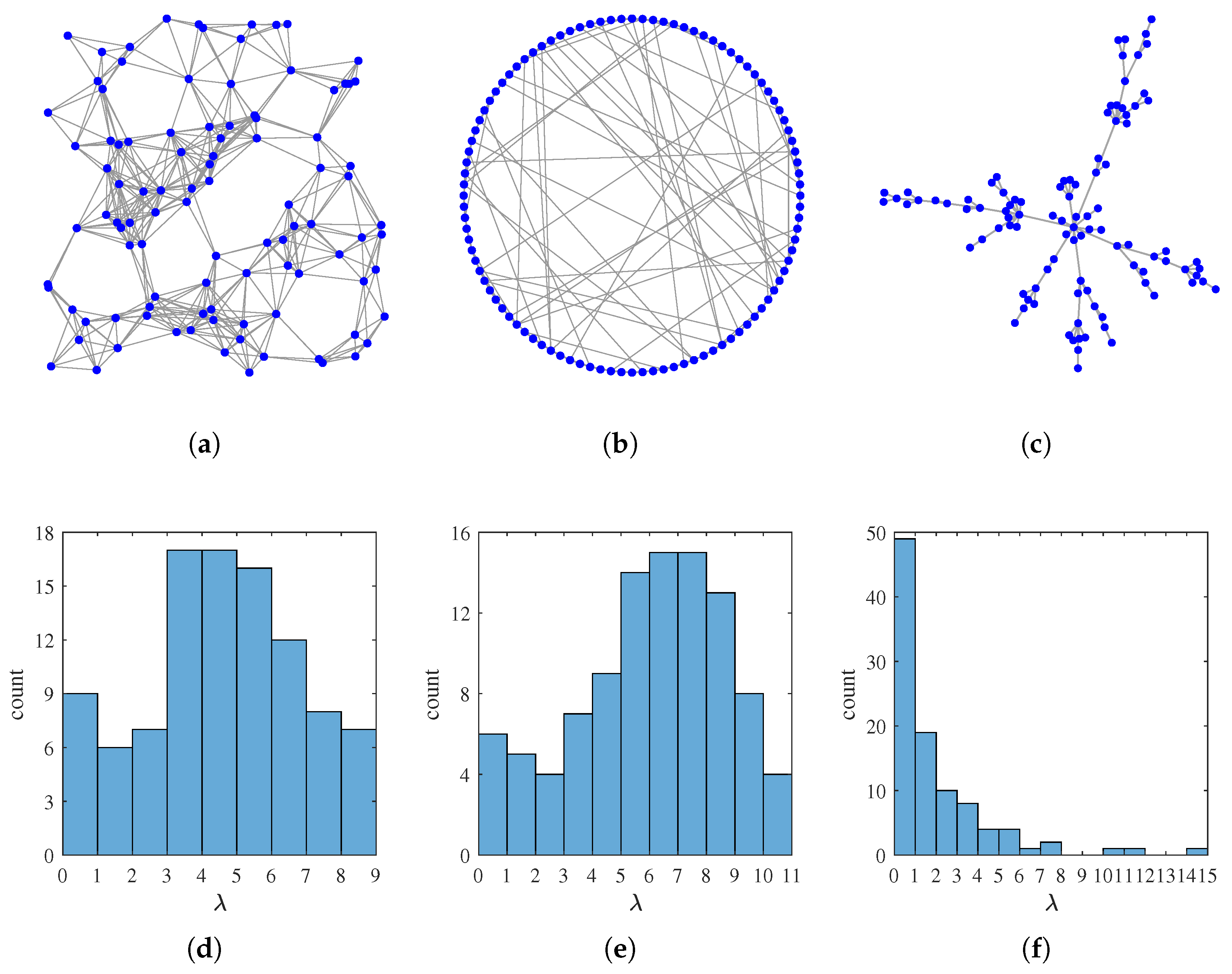
Three graphs of representative types that have widespread applications in the real world are used for testing in our experiments:

• ${\mathcal{G}}_1$: A random geometric graph with $N=100$ vertices randomly placed in a 1-by-1 square, and edge weights assigned via a thresholded Gaussian kernel

  $$w_{ij}=\left\{\begin{array}{cc}exp\left(-{\displaystyle \frac{d_{ij}^2}{2{\sigma }^2}}\right),\hfill & \mathrm{if}{d}_{ij}<r\hfill \\ 0,\hfill & \mathrm{otherwise}\hfill \end{array}\right.$$

  (27)

  where $d_{ij}$ is the Euclid distance between vertex i and vertex j, $r=0.2$ and $\sigma =0.1$.
• ${\mathcal{G}}_2$: A small world graph with $N=100$ nodes, generated by the Watts–Strogatz model [32] with mean node degree 6 and rewiring probability $0.2$.
• ${\mathcal{G}}_3$: A scale-free graph with $N=100$ nodes, generated by the Barabási–Albert model [33,34] with 1 initial node, each newly added node connected to 1 existing node, and connecting probabilities proportional to the degrees of existing nodes.

The graph topologies as well as their eigenvalue distributions are visualized in Figure 1. Due to limited space, we will mainly display and analyze our experimental results on ${\mathcal{G}}_1$ in detail, whereas example results on ${\mathcal{G}}_2$ and ${\mathcal{G}}_3$ are shown at the end to demonstrate the topology adaptability.

Graph signals are generated from the ABL prior distribution Equation (1). Moreover, observation noise follows i.i.d. zero-mean Gaussian distribution Equation (6). A variety of hyperparameters are considered, in order to cover ABL graph signals with different bandwidth, strictness of bandlimitedness and energy level, and scenarios with different signal-noise ratio (SNR). SNR here considering random ABL graph signal is defined as

$${SNR}_{\mathrm{r}}=10lg{\displaystyle \frac{{\sum }_{k=1}^{N}1/(\alpha +\gamma {\lambda }_k^{2n})}{N/\beta }}.$$

(28)

For each setting, 100 graph signals are generated to evaluate the average performance of each method. The average estimation errors under different sample sizes are computed and plotted.

First of all, we compare the performance of the proposed algorithm with RndEM and OrcUS on ${\mathcal{G}}_1$. Hyperparameters are set to $n=2$, ${\lambda }_{\mathrm{c}}=2$, $g=1$, and ${SNR}_{\mathrm{r}}=15$dB. As shown in Figure 2, although in the initial stage, the estimation error of the proposed algorithm is similar to RndEM, as the sample size grows, our performance gradually approaches that of OrcUS. This result is as expected, as hyperparameter estimation gets better with growing sample size, which can lead to more efficient sample selection and more accurate signal estimation. Our superiority to RndEM (EM estimation without US sampling) demonstrates the effectiveness of choosing sampling nodes by US. The performance gap between our method and OrcUS (US sampling with known hyperparameters) tends to disappear when samples are abundant, also supporting the validity of hyperparameter estimation by EM.

Subsequently, the proposed algorithm is compared to three existing sampling and estimation methods—Anis2016, Perraudin2018, and Sakiyama2019—in scenarios without much prior knowledge about signal and noise model. A series of experiments with different hyperparameters are done on ${\mathcal{G}}_1$ to test and compare their performance in all kinds of settings. In the first experiment, we fix $g=1$, ${SNR}_{\mathrm{r}}=15$dB, and repeat the simulation with $n=1,2$, ${\lambda }_{\mathrm{c}}=2,3$, corresponding to ABL graph signals with different bandwidth and strictness of bandlimitedness. Simulation results are depicted in Figure 3. From the graphics we can see, the proposed algorithm can obtain better or competitive estimation performance compared to state-of-the-art methods on ABL graph signals with various properties. For Perraudin2018 and Sakiyama2019, the proposed method significantly outperforms them after a small number of initial samples in all the four settings. As for Anis2016, when n is small or ${\lambda }_{\mathrm{c}}$ is large, which means the signal is far from strictly bandlimited or occupies large bandwidth, we need far fewer samples than Anis2016 to recover the signal with tolerable error. This is because our method estimates the graph signal at all frequencies from the beginning thanks to the Bayesian framework, and our signal prior with hyperparameters estimated from data can better fit ABL graph signals with different properties. Therefore, the proposed algorithm is more robust against different signal properties and is able to obtain better estimation results in most cases.

We continue to investigate our performance for ABL graph signals with different energy level as well as in scenarios with different signal–noise ratio. We fix $n=2$, ${\lambda }_{\mathrm{c}}=2$. When changing g from 0.01 to 100, ${SNR}_{\mathrm{r}}$ is fixed at 15 dB. When changing ${SNR}_{\mathrm{r}}$ from 5 dB to 25 dB, g is fixed at 1. Sampling size is set to $M=60$. According to Figure 4a, the proposed algorithm gets better performance for graph signals with lower energy. For one thing, even though the estimated variance in the signal prior also becomes larger when the signal energy is larger, the zero-mean Gaussian prior still prefers signals with lower energy. For another, as the variance gets larger, the signal prior becomes flatter, and thus weaker, in the sense that it has less preference among different signals. Therefore, more observations are needed to reach the same estimation accuracy. Fortunately, this problem can be overcome by adaptive rescaling, dividing the observed signal values by a sufficiently large number, as long as we know the rough order of magnitudes of the signal energy. As for SNR, from Figure 4b, although lower SNR may result in worse performance of the proposed algorithm, our method keeps outperforming the others when samples are adequate.

Then, example simulation results on ${\mathcal{G}}_2$ and ${\mathcal{G}}_3$ are given in Figure 5. $n=2$, $g=1$, ${SNR}_{\mathrm{r}}=15$ dB. ${\lambda }_{\mathrm{c}}=3$ for ${\mathcal{G}}_2$, and ${\lambda }_{\mathrm{c}}=1$ for ${\mathcal{G}}_3$. The proposed algorithm also reaches higher estimation accuracy than the other methods with enough sampling budget. This demonstrates the robustness of the proposed algorithm against different graph topologies.

From the simulation results above, without much prior knowledge, the proposed algorithm can adjust to ABL graph signals with different bandwidth, strictness of bandlimitedness, energy level, and SNR. In most cases, exceeding a small number of initial samples, the proposed algorithm is able to estimate the graph signals with higher accuracy than the existing methods.

Besides the validation of the limited-budget performance, we also verify the consistency of the proposed algorithm by a simulation experiment. We generate an ABL graph signal on ${\mathcal{G}}_1$ with $n=2$, ${\lambda }_{\mathrm{c}}=2$, and $g=1$, and the SNR is set to $15\mathrm{dB}$. To observe the asymptotic performance, the maximum sample size is set to ${10}^5$, which is ${10}^3$ times the graph size. We repeat the proposed algorithm on the graph signal for 50 times to see the mean as well as the variance of the estimation errors.

As shown in Figure 6, the mean normalized $l_2$-norm error tends to decrease continuously as the sample size grows, and has decreased to about $5\times {10}^{-3}$ when the sample size reaches ${10}^5$. The standard deviation also tends to decline with growing sample size, which is around $3\times {10}^{-4}$ with ${10}^5$ samples. Other ABL graph signals also have similar results. This agrees with the consistency of the proposed algorithm, which has been stated and theoretically proved in Section 4.

5.2. A Real-World Example of Temperature Sensor Network

As an application example, we apply the proposed algorithm to the air temperatures measured by weather stations in China [35]. This example shows a potential application of the proposed algorithm in sensor selection.

We construct a K-nearest neighbor (K-NN) graph from the $N=381$ weather stations with $K=5$, where each node corresponds to a weather station, and the great-circle distances between stations are considered in K-NN search. Edge weights are assigned via a Gaussian kernel:

$$w_{ij}=exp\left(-{\displaystyle \frac{d_{ij}^2}{2{\sigma }^2}}\right)\mathrm{for}(i,j)\in \mathcal{E},$$

(29)

where $d_{ij}$ is the great-circle distance between station i and station j in degree, and $\sigma =2$.

Then, the air temperatures measured by these weather stations can be seen as a graph signal. We consider two such signals in our experiment: ${\mathit{f}}_1$ at 0:00 on 1 January 2020, which is a winter night, and ${\mathit{f}}_2$ at 12:00 on 1 July 2020, which is a summer noon. The two graph signals and their spectra are visualized in Figure 7. As expected, the signals are smooth in the vertex domain and approximately bandlimited in the frequency domain.

We apply the proposed sequential sampling and estimation algorithm to these graph signals. Additive i.i.d. zero-mean Gaussian observation noise following Equation (6) is added, where ${SNR}_{\mathrm{d}}=10lg{\displaystyle \frac{{\mathit{f}}^T\mathit{f}}{N/\beta }}$ is 15 dB. The known hyperparameter n in the signal prior Equation (1) is set to $1/2$, which means a smoothness prior Equation (3) is considered. The observed signal values are divided by 100 as preprocessing, and accordingly the estimated graph signal is multiplied by 100 at output. The performance of the proposed algorithm is compared to Anis2016, Perraudin2018 and Sakiyama2019. As our first sampling node is chosen at random, Perraudin2018 is a random sampling method, and the observation noises also introduce randomness, we test each method on the same signal for 20 times, and compare their average estimation errors.

As shown in Figure 8, although the proposed algorithm needs some initial samples to “warm up”, after that the estimation error decreases rapidly and surpass Anis2016, Perraudin2018, and Sakiyama2019 in very short time, and we keep leading as the sample size further grows. This is because our sequential method with unknown hyperparameters requires a certain number of samples to have a relatively proper estimation of the signal and noise distributions. Then, based on the latest signal bandwidth, energy level, and noise precision estimated from data, we are able to choose the subsequent sampling nodes more efficiently and estimate the graph signal more accurately than other methods that take no account of such signal and noise properties.

6. Conclusions

In this paper, a sequential sampling and estimation algorithm is proposed for approximately bandlimited graph signals without complete prior knowledge about signal and noise properties. In the proposed algorithm, hyperparameter estimation by EM based on historical observations and sample selection by US with latest estimated hyperparameters are done in an alternating way. We prove in theory the consistency of signal estimation in the proposed algorithm under specific conditions. Finite-time performance of the proposed algorithm is validated by a series of simulation results. The proposed method provides a novel and practical sequential framework for graph signal sampling with unknown hyperparameters in the system model, and the experiment on temperature data shows our potential application in sensor selection on sensor networks with smooth measurements over the topologies. Other potential applications include opinion prediction in social networks assuming that people with strong social connection are likely to hold similar opinions, and active semisupervised learning tasks on similarity graphs.

References

1. Shuman, D.I.; Narang, S.K.; Frossard, P.; Ortega, A.; Vandergheynst, P. The emerging field of signal processing on graphs: Extending high-dimensional data analysis to networks and other irregular domains. IEEE Signal Process. Mag. 2013, 30, 83–98. [Google Scholar] [CrossRef] [Green Version]
2. Sandryhaila, A.; Moura, J.M.F. Discrete signal processing on graphs. IEEE Trans. Signal Process. 2013, 61, 1644–1656. [Google Scholar] [CrossRef] [Green Version]
3. Shuman, D.I.; Vandergheynst, P.; Frossard, P. Chebyshev polynomial approximation for distributed signal processing. In Proceedings of the 2011 International Conference on Distributed Computing in Sensor Systems and Workshops (DCOSS), Barcelona, Spain, 27–29 June 2011. [Google Scholar]
4. Shi, X.; Feng, H.; Zhai, M.; Yang, T.; Hu, B. Infinite impulse response graph filters in wireless sensor networks. IEEE Signal Process. Lett. 2015, 22, 1113–1117. [Google Scholar] [CrossRef]
5. Loukas, A.; Simonetto, A.; Leus, G. Distributed autoregressive moving average graph filters. IEEE Signal Process. Lett. 2015, 22, 1931–1935. [Google Scholar] [CrossRef] [Green Version]
6. Chen, S.; Varma, R.; Sandryhaila, A.; Kovačević, J. Discrete signal processing on graphs: Sampling theory. IEEE Trans. Signal Process. 2015, 63, 6510–6523. [Google Scholar] [CrossRef] [Green Version]
7. Anis, A.; Gadde, A.; Ortega, A. Efficient sampling set selection for bandlimited graph signals using graph spectral proxies. IEEE Trans. Signal Process. 2016, 64, 3775–3789. [Google Scholar] [CrossRef]
8. Narang, S.K.; Gadde, A.; Ortega, A. Signal processing techniques for interpolation in graph structured data. In Proceedings of the 2013 IEEE International Conference on Acoustics, Speech and Signal Processing (ICASSP), Vancouver, BC, Canada, 26–31 May 2013; pp. 5445–5449. [Google Scholar]
9. Sakiyama, A.; Tanaka, Y.; Tanaka, T.; Ortega, A. Efficient sensor position selection using graph signal sampling theory. In Proceedings of the 2016 IEEE International Conference on Acoustics, Speech and Signal Processing (ICASSP), Shanghai, China, 20–25 March 2016; pp. 6225–6229. [Google Scholar]
10. Jabłoński, I. Graph signal processing in applications to sensor networks, smart grids, and smart cities. IEEE Sens. J. 2017, 17, 7659–7666. [Google Scholar] [CrossRef]
11. Huang, W.; Bolton, T.A.W.; Medaglia, J.D.; Bassett, D.S.; Ribeiro, A.; Ville, D.V.D. A graph signal processing perspective on functional brain imaging. Proc. IEEE 2018, 106, 868–885. [Google Scholar] [CrossRef]
12. Cheung, G.; Magli, E.; Tanaka, Y.; Ng, M.K. Graph spectral image processing. Proc. IEEE 2018, 106, 907–930. [Google Scholar] [CrossRef] [Green Version]
13. Dinesh, C.; Cheung, G.; Bajić, I.V. Point cloud denoising via feature graph Laplacian regularization. IEEE Trans. Image Process. 2020, 29, 4143–4158. [Google Scholar] [CrossRef] [PubMed]
14. Gadde, A.; Anis, A.; Ortega, A. Active semi-supervised learning using sampling theory for graph signals. In Proceedings of the 20th ACM SIGKDD International Conference on Knowledge Discovery and Data Mining, New York, NY, USA, 24–27 August 2014; pp. 492–501. [Google Scholar]
15. Anis, A.; El Gamal, A.; Avestimehr, A.S.; Ortega, A. A sampling theory perspective of graph-based semi-supervised learning. IEEE Trans. Inf. Theory 2019, 65, 2322–2342. [Google Scholar] [CrossRef] [Green Version]
16. Kipf, T.N.; Welling, M. Semi-supervised classification with graph convolutional networks. In Proceedings of the 5th International Conference on Learning Representations (ICLR), Palais des Congrès Neptune, Toulon, France, 24–26 April 2017. [Google Scholar]
17. Chen, S.; Varma, R.; Singh, A.; Kovačević, J. Signal recovery on graphs: Fundamental limits of sampling strategies. IEEE Trans. Signal Inf. Process. Netw. 2016, 2, 539–554. [Google Scholar] [CrossRef] [Green Version]
18. Puy, G.; Tremblay, N.; Gribonval, R.; Vandergheynst, P. Random sampling of bandlimited signals on graphs. Appl. Comput. Harmon. Anal. 2018, 44, 446–475. [Google Scholar] [CrossRef] [Green Version]
19. Xie, X.; Feng, H.; Jia, J.; Hu, B. Design of sampling set for bandlimited graph signal estimation. In Proceedings of the 2017 IEEE Global Conference on Signal and Information Processing (GlobalSIP), Montreal, QC, Canada, 14–16 November 2017; pp. 653–657. [Google Scholar]
20. Lin, S.; Xie, X.; Feng, H.; Hu, B. Active sampling for approximately bandlimited graph signals. In Proceedings of the 2019 IEEE International Conference on Acoustics, Speech and Signal Processing (ICASSP), Brighton, UK, 12–17 May 2019; pp. 5441–5445. [Google Scholar]
21. Perraudin, N.; Ricaud, B.; Shuman, D.I.; Vandergheynst, P. Global and local uncertainty principles for signals on graphs. APSIPA Trans. Signal Inf. Process. 2018, 7, e3. [Google Scholar] [CrossRef] [Green Version]
22. Xie, X.; Yu, J.; Feng, H.; Hu, B. Bayesian design of sampling set for bandlimited graph signals. In Proceedings of the 2019 IEEE Global Conference on Signal and Information Processing (GlobalSIP), Ottawa, ON, Canada, 11–14 November 2019. [Google Scholar]
23. Gadde, A.; Ortega, A. A probabilistic interpretation of sampling theory of graph signals. In Proceedings of the 2015 IEEE International Conference on Acoustics, Speech and Signal Processing (ICASSP), South Brisbane, Australia, 19–24 April 2015; pp. 3257–3261. [Google Scholar]
24. Bishop, C.M. Pattern Recognition and Machine Learning; Springer: New York, NY, USA, 2006; ISBN 9780387310732. [Google Scholar]
25. Settles, B. Active Learning; Morgan & Claypool: San Rafael, CA, USA, 2012; ISBN 9781608457250. [Google Scholar]
26. Bernardo, J.M.; Smith, A.F.M. Bayesian Theory; John Wiley & Sons: Hoboken, NJ, USA, 1994; ISBN 0471924164. [Google Scholar]
27. Petrone, S.; Rousseau, J.; Scricciolo, C. Bayes and empirical Bayes: Do they merge? Biometrika 2014, 101, 285–302. [Google Scholar] [CrossRef] [Green Version]
28. Pronzato, L. One-step ahead adaptive D-optimal design on a finite design space is asymptotically optimal. Metrika 2010, 71, 219–238. [Google Scholar] [CrossRef] [Green Version]
29. Oppenheim, A.V.; Schafer, R.W. Discrete-Time Signal Processing, 3rd ed.; Prentice Hall: Englewood Cliffs, NJ, USA, 2009; ISBN 9780136024552. [Google Scholar]
30. Kay, S.M. Fundamentals of Statistical Signal Processing, Volume I: Estimation Theory; Prentice Hall: Englewood Cliffs, NJ, USA, 1993; ISBN 9780133457117. [Google Scholar]
31. Sakiyama, A.; Tanaka, Y.; Tanaka, T.; Ortega, A. Eigendecomposition-free sampling set selection for graph signals. IEEE Trans. Signal Process. 2019, 67, 2679–2692. [Google Scholar] [CrossRef] [Green Version]
32. Watts, D.J.; Strogatz, S.H. Collective dynamics of ‘small-world’ networks. Nature 1998, 393, 440–442. [Google Scholar] [CrossRef] [PubMed]
33. Barabási, A.L.; Albert, R. Emergence of scaling in random networks. Science 1999, 286, 509–512. [Google Scholar] [CrossRef] [PubMed] [Green Version]
34. Perraudin, N.; Paratte, J.; Shuman, D.; Martin, L.; Kalofolias, V.; Vandergheynst, P.; Hammond, D.K. GSPBOX: A toolbox for signal processing on graphs. arXiv 2016, arXiv:1408.5781v2 [cs.IT]. [Google Scholar]
35. Integrated Surface Database (ISD) by National Climatic Data Center (NCDC) of the USA. Available online: https://www.ncdc.noaa.gov/isd (accessed on 11 December 2020).
Figure 1. The three graphs used in our simulations, and the histograms of their eigenvalue distributions. (a) G 1 , a random geometric graph and (d) its eigenvalue distribution. (b) G 2 , a Watts–Strogatz small world graph and (e) its eigenvalue distribution. (c) G 3 , a Barabási–Albert scale-free graph and (f) its eigenvalue distribution.
Sensors 21 01460 g001
Figure 2. Estimation error with growing sample size of the proposed algorithm versus RndEM and OrcUS on G 1 . Hyperparameters are n = 2 , λ c = 2 , g = 1 , and S N R r = 15 dB.
Sensors 21 01460 g002
Figure 3. Estimation errors of the proposed algorithm versus Anis2016, Perraudin2018, and Sakiyama2019 on G 1 with different signal bandwidth and strictness of bandlimitedness, i.e., different n and λ c . We fix g = 1 and S N R r = 15 dB. (a) n = 1 , λ c = 2 . (b) n = 1 , λ c = 3 . (c) n = 2 , λ c = 2 . (d) n = 2 , λ c = 3 .
Sensors 21 01460 g003
Figure 4. Estimation errors of the proposed algorithm versus Anis2016, Perraudin2018, and Sakiyama2019 on G 1 with different signal energy level and signal–noise ratio, i.e., different g and S N R r . We fix n = 2 , λ c = 2 . The sampling size is set to M = 60 . (a) g is changed from 0.01 to 100, while S N R r is fixed at 15 dB. (b) S N R r is changed from 5 dB to 25 dB, while g is fixed at 1.
Sensors 21 01460 g004
Figure 5. Estimation errors of the proposed algorithm versus Anis2016, Perraudin2018, and Sakiyama2019 on G 2 and G 3 . (a) Results on G 2 with n = 2 , λ c = 3 , g = 1 , S N R r = 15 dB. (b) Results on G 3 with n = 2 , λ c = 1 , g = 1 , S N R r = 15 dB.
Sensors 21 01460 g005
Figure 6. Result of the consistency verification experiment. The graph signal is on G 1 generated with n = 2 , λ c = 2 , g = 1 , and the observation SNR is 15 dB . The curve denotes the mean of the normalized l 2 -norm error, and the region corresponds to ± 1 standard deviation around the mean. In the overview figure, the y-axis is in logarithmic scale to better display the decrease of the mean estimation error, whereas in the partial enlargement, it is linear to present the decline of the standard deviation.
Sensors 21 01460 g006
Figure 7. Two graph signals of air temperatures measured by 381 weather stations in China, and their spectra. (a) f 1 at 0:00 on 1 January 2020, and (b) its spectrum. (c) f 2 at 12:00 on 1 July 2020, and (d) its spectrum.
Sensors 21 01460 g007
Figure 8. Estimation errors of the two temperature graph signals by the proposed algorithm versus Anis2016, Perraudin2018, and Sakiyama2019. (a) Results on f 1 . (b) Results on f 2 .
Sensors 21 01460 g008
Publisher’s Note: MDPI stays neutral with regard to jurisdictional claims in published maps and institutional affiliations.