1. Introduction
As a significant technology for noncooperative wireless communication systems, automatic modulation recognition (AMR) plays an important role in practical civil and military applications, such as cognitive radio, interference recognition and spectrum monitoring [
1]. In the absence of prior knowledge, it can identify the modulation type of an intercepted signal, providing parameter information for subsequent demodulation [
2].
Traditional AMR algorithms can be divided into two categories. One is based on maximum likelihood (ML) theory [
3], and the other is a feature-based (FB) method [
4]. The first approach uses probability theory, hypothesis test theory and an appropriate decision strategy to solve the AMR problem. The feature-based approach first extracts the modulated signal characteristics and then completes the recognition using classifiers. In feature-based methods, the number of selected features influences the recognition performance. The main features used for modulation signal identification include instantaneous amplitude, phase, frequency, high-order cumulant [
5], cyclic spectrum [
6] and wavelet characteristics [
7]. Many of the classifiers used are based on machine learning algorithms; these include decision trees, support vector machines (SVMs) [
8] and artificial neural networks (ANNs) [
9].
In recent years, deep learning (DL), which is a powerful machine learning approach, has achieved great success in diverse fields such as image classification [
10] and speech recognition [
11]. The concept of DL comes from the research of ANNs. A multilayer perceptron with multiple hidden layers is a DL structure. DL forms a more abstract high-level representation attribute category or feature by combining low-level features to discover distributed feature representations of data. Its goal is to allow machines to have the ability to analyze and learn similar to humans and recognize data such as text, images and sounds. DL solves nonlinear classification problems by using activation functions and uses regularization to improve the robustness of the model [
12]. The DL-based methods cascade multilayer nonlinear processing units to extract features. This approach can automatically optimize the extracted features to minimize later classification errors.
Many scholars have applied DL to the field of AMR in recent years. For example, Lee et al. [
13] proposed a new method that calculated 28 statistical characteristics of five modulation signals; these were then sent to a fully connected feedforward network to conduct classification. Wang Yu at al. [
14] trained CNN on samples composed of in-phase and quadrature component signals to distinguish modulation patterns that are relatively easy to identify. At the same time, a CNN based on the constellation map was designed to identify modulation modes that were difficult to distinguish in previous CNNs and improved the ability to classify QAM signals under low SNRs. Li et al. [
12] studied the AMR method based on the original IQ signal under the parameter estimation error. First, the influence of parameter estimation error on the performance of CNN classifier is analyzed. Then, an AMR method based on spatial transformation network (STN) is proposed, which improves the robustness under parameter estimation errors. Li et al. [
15] proposed a deep joint learning algorithm based on CNN and kernel collaborative representation and discriminative projection (KCRDP), including deep learning and kernel dictionary learning, which improves the adaptability of small samples and reduces the computational complexity without prior knowledge and feature enhancement processing.
In 2016, O’Shea et al. [
16] generated a public dataset of modulated signals, named RML2016.10a, using GNU Radio software; then, they used a convolutional neural network (CNN) to identify the modulated signals. Subsequent studies have also adopted this dataset for AMR research. That same year, O’Shea [
17] proposed a method to optimize the CNN structure. West et al. [
18] applied a CNN, a residual network (Resnet), a convolutional long short-term memory deep neural network (CLDNN) and an Inception network to the modulated signal identification task and compared their respective recognition performances. The results show that the modulation signal recognition performance is not solely dependent on the network depth. Zhang et al. [
19] proposed a preprocessing signal representation that combined the in-phase, quadrature and fourth-order statistics of the modulated signals. Omar S. Mossad et al. [
20] proposed a CNN that used a multitask learning scheme (MTL-CNN) to reduce the confusion between similar classes. Kumar et al. [
21] introduced a signal distortion correction module (CM) to estimate the carrier frequency offset and phase noise of the received signal to improve modulation recognition accuracy of deep learning schemes. Liu [
22] proposed a group lasso based lightweight DNN for AMR which can learn to prune via automatically removing the neurons in hidden layers.
In 2020, Jakob et al. [
23] used a linear combination to enable the DL architecture to perform complex convolutions (CVCs) and learn the characteristics of the real and imaginary parts of modulated signals. Wu et al. [
24] constructed a CNN followed by a long short-term memory (LSTM) model as the classifier (CNN-LSTM) to efficiently explore the temporal and spatial correlation. However, to the best of our knowledge, none of the currently available methods fully consider the phase and contextual information of the modulated signals simultaneously.
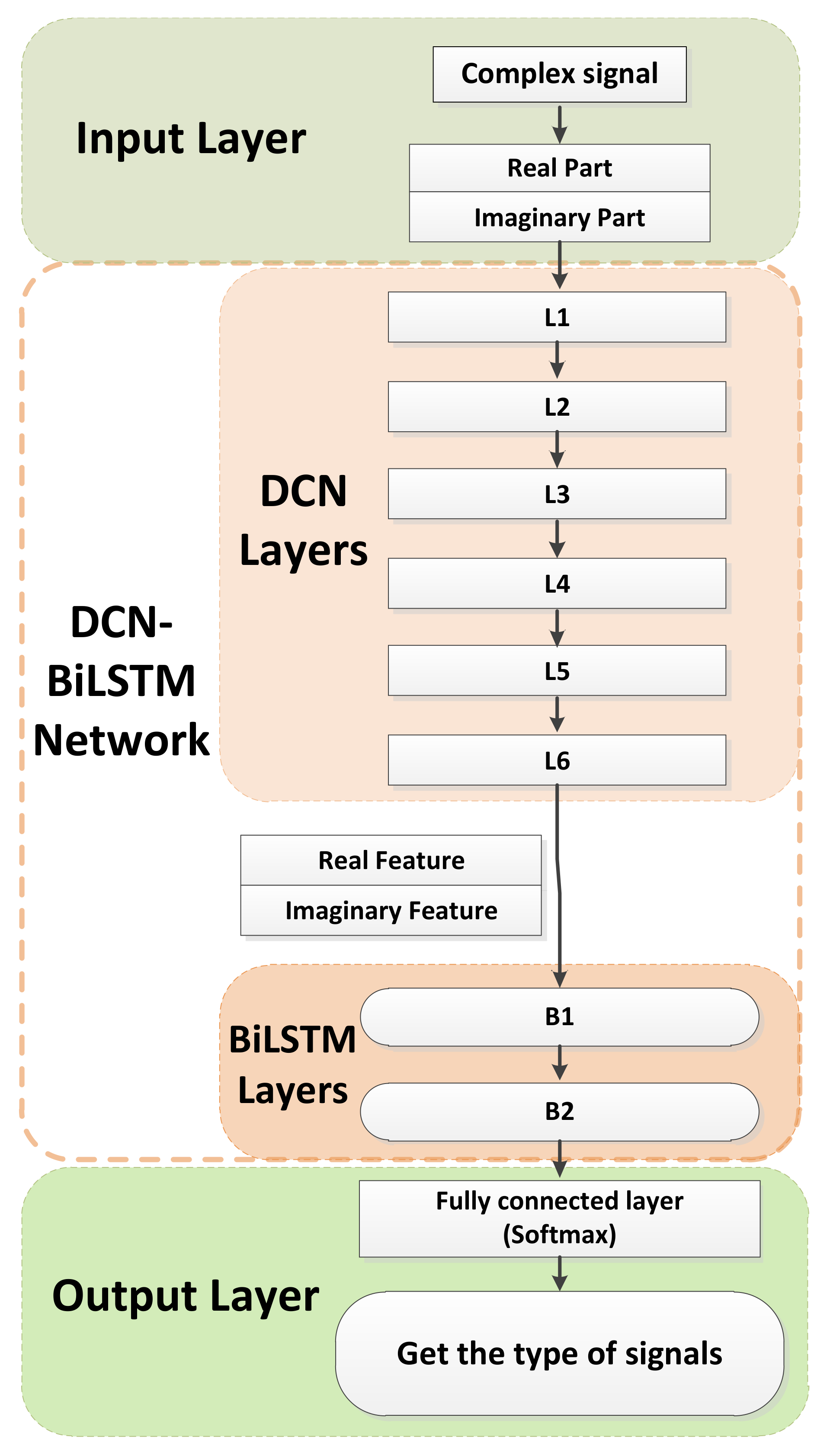
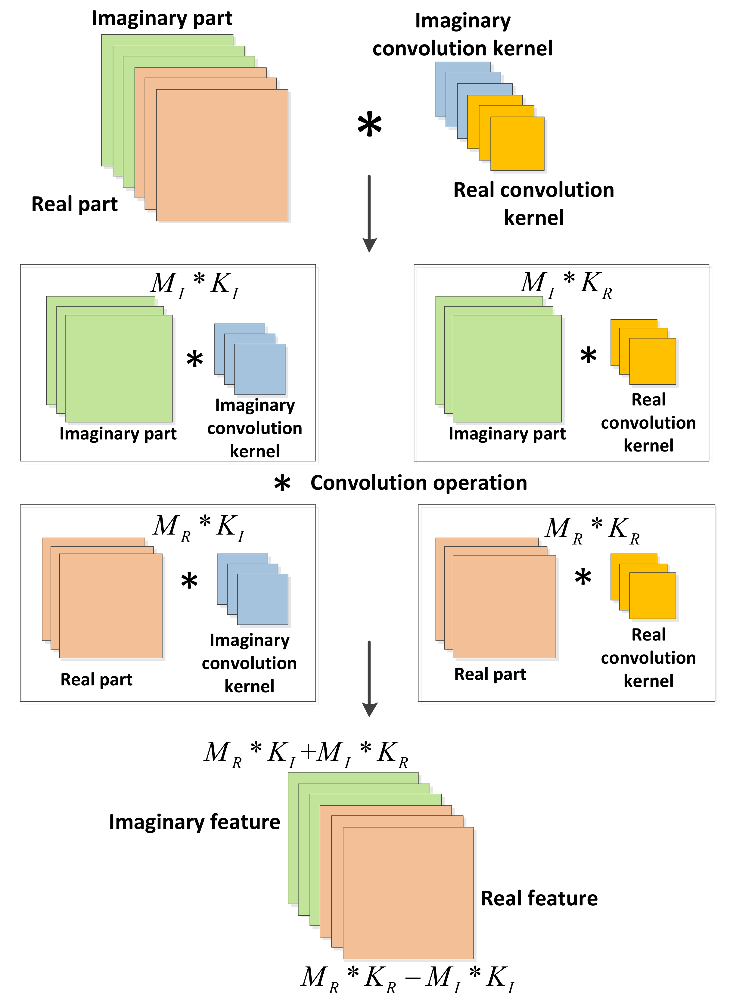
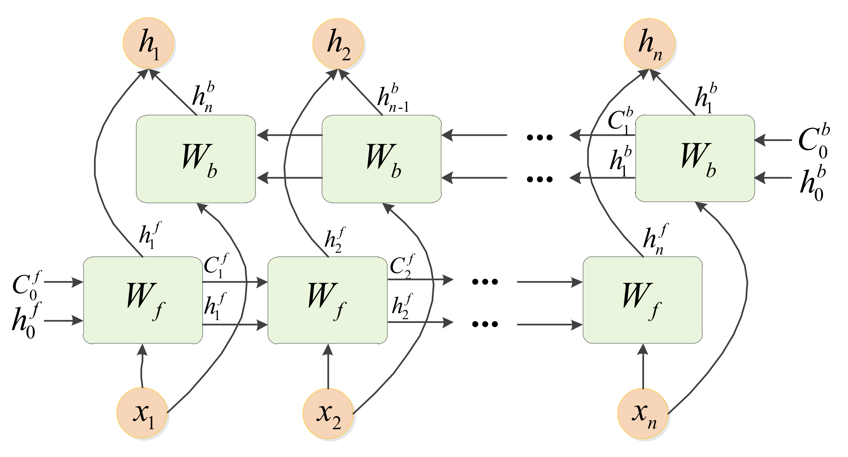
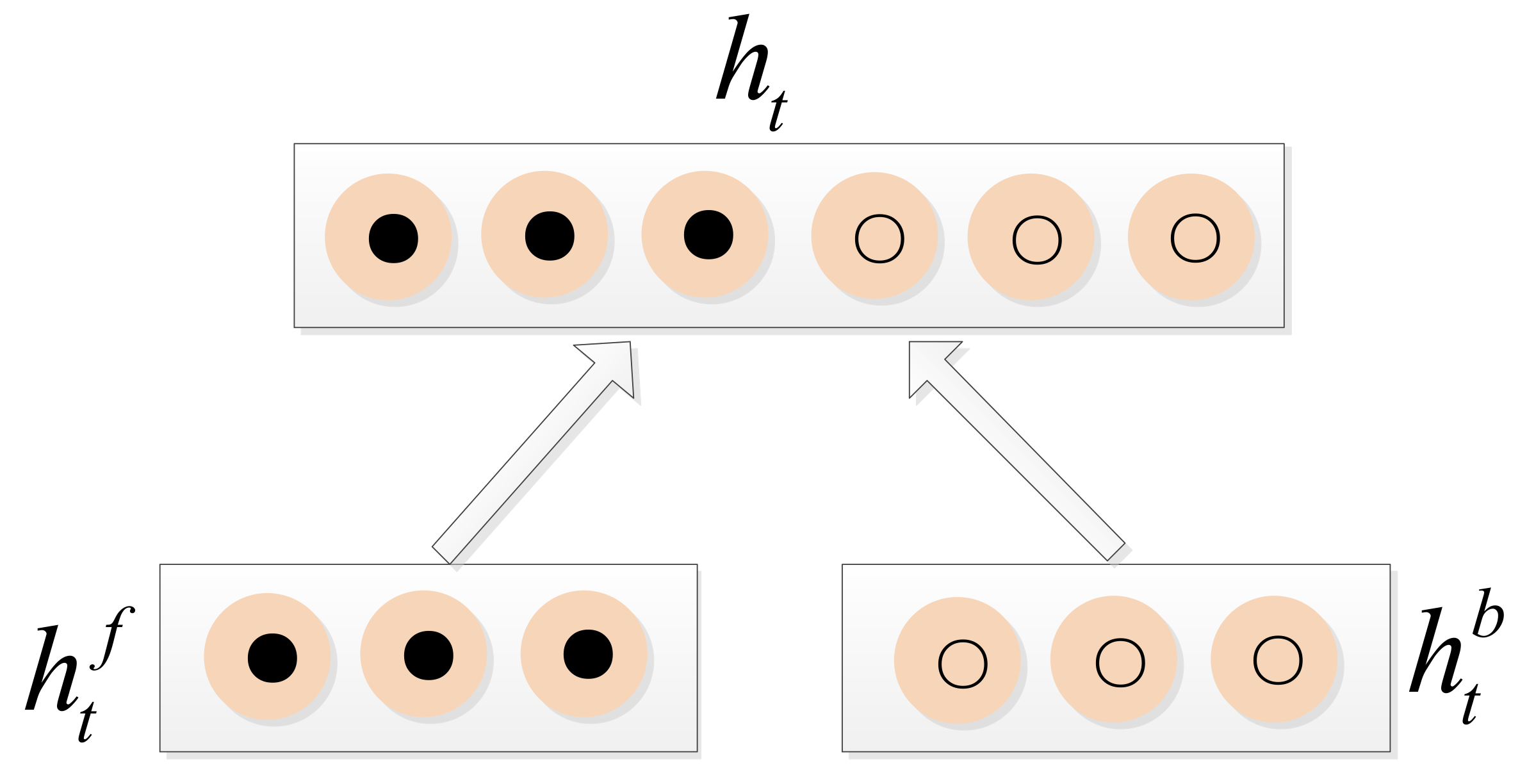
In view of the current problems, this paper proposes a deep complex network that cascades bidirectional long short-term memory network (DCN-BiLSTM). First, deep complex network (DCN) layers with convolution kernels of different scales are connected; then, the bidirectional long short- term memory (BiLSTM) layers are cascaded. Finally, a softmax classifier is used to classify 11 kinds of digitally modulated signals. The main contributions of this paper are as follows:
- (1)
To the best of our knowledge, this study is the first to cascade DCN and BiLSTM models and apply them in the AMR field.
- (2)
We demonstrate the effectiveness of the DCN-BiLSTM network through experiments. The experimental results show that the performance of the proposed algorithm is better than that of other neural network recognition algorithms. When the signal-to-noise ratio (SNR) exceeds 4 dB, the recognition rate of our proposed model on the 11 modulation signals can reach 90%.
The remainder of this paper is organized as follows.
Section 2 shows the signal model.
Section 3 proposes the DCN-BiLSTM network model and introduces its components. In
Section 4, we report the results of an experiment conducted to evaluate the proposed method and provide the optimal parameter configuration for the DCN-BiLSTM model. In addition, we use a cross-validation method to evaluate the network. Finally,
Section 5 concludes this paper.
2. Signal Model
This paper uses the open dataset named RML2016.10a [
16].
Figure 1 illustrates the dataset generation technique used in [
16]. For the Rayleigh fading channel, the received signal can be expressed as
where
is the modulated signal sent by the communication transmitter and
L is the number of multipaths;
is the Rayleigh fading factor of the
lth path;
is the delay of the
lth path;
represents the Doppler frequency; and
is additive white Gaussian noise. In addition, to ensure that the channel model is similar to a real channel, the channel model of this dataset includes the sampling rate and carrier rate offsets. The specific modulation types and parameters are shown in
Table 1.
For a received signal, if we know the modulation type range, sampling frequency, sampling rate offset range, carrier rate offset range and the other signal parameters included in
Table 1, we can use the recognition system model proposed in
Section 3.
4. Experiment Results and Discussions
The relevant platform and software settings for this experiment are shown in
Table 2. There are 1000 samples of each modulated signal for each SNR comprising a total of samples is 220,000 samples. The ratio of training sets to test sets is 8:2. We use the np.random.choice function to implement the proportional selection of the dataset to obtain the training sets and the test sets. In this experiment, we performed the following steps.
Initialize the DCN-BiLSTM network randomly, extract a specified number of samples in the training sets and input them into the network for training.
Compare the classification result obtained in the last layer of the network with the actual type; use the cross-entropy function to calculate the network loss value; and adjust the network weight value through the optimization algorithm.
Before the next training starts, use the loss value as a standard to measure the network performance. When it does not drop within 10 iterations, the training is stopped.
Repeat Steps 2–4 until the maximum number of training is reached or the conditions for premature termination of training are met. The maximum number of training in this article is 150. After training, the weights are saved and the classification model is output.
Input the test sets into the trained model to obtain the recognition result.
4.1. Algorithm Performance Comparison
We selected the recognition algorithms based on a CNN [
17], Resnet [
18], Inception [
18], CLDNN [
18], MTL-CNN [
20], CVC [
23] and CNN-LSTM [
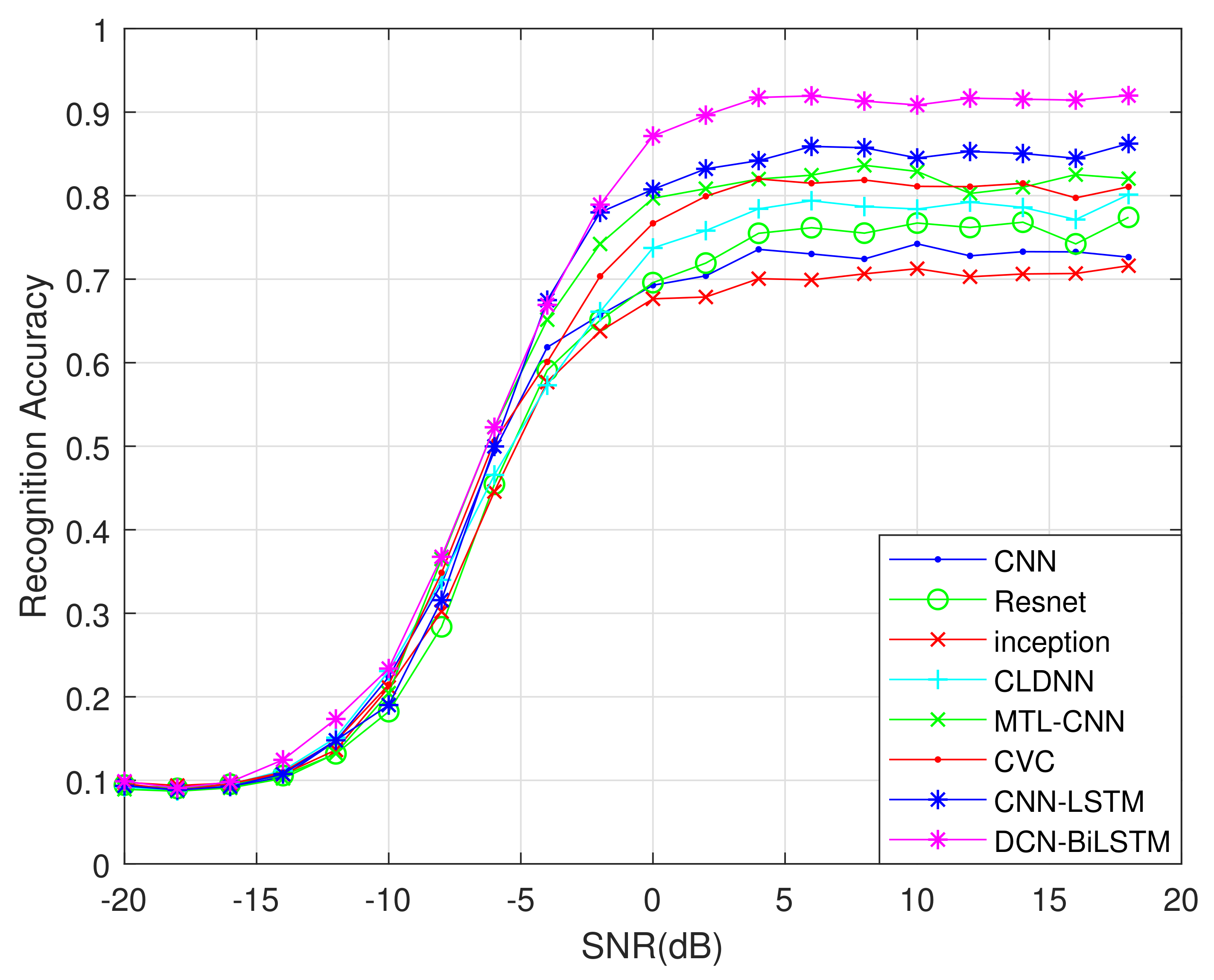
24] as benchmark models. A performance comparison chart for these eight recognition algorithms is shown in
Figure 8.
Figure 8 shows that, from −2 to 18 dB, the accuracy of the DCN-BiLSTM network is substantially higher than the accuracy of the other seven recognition algorithms. When the SNR exceeds 4 dB, the recognition accuracy of the DCN-BiLSTM network for the 11 modulation signals can reach 90%.
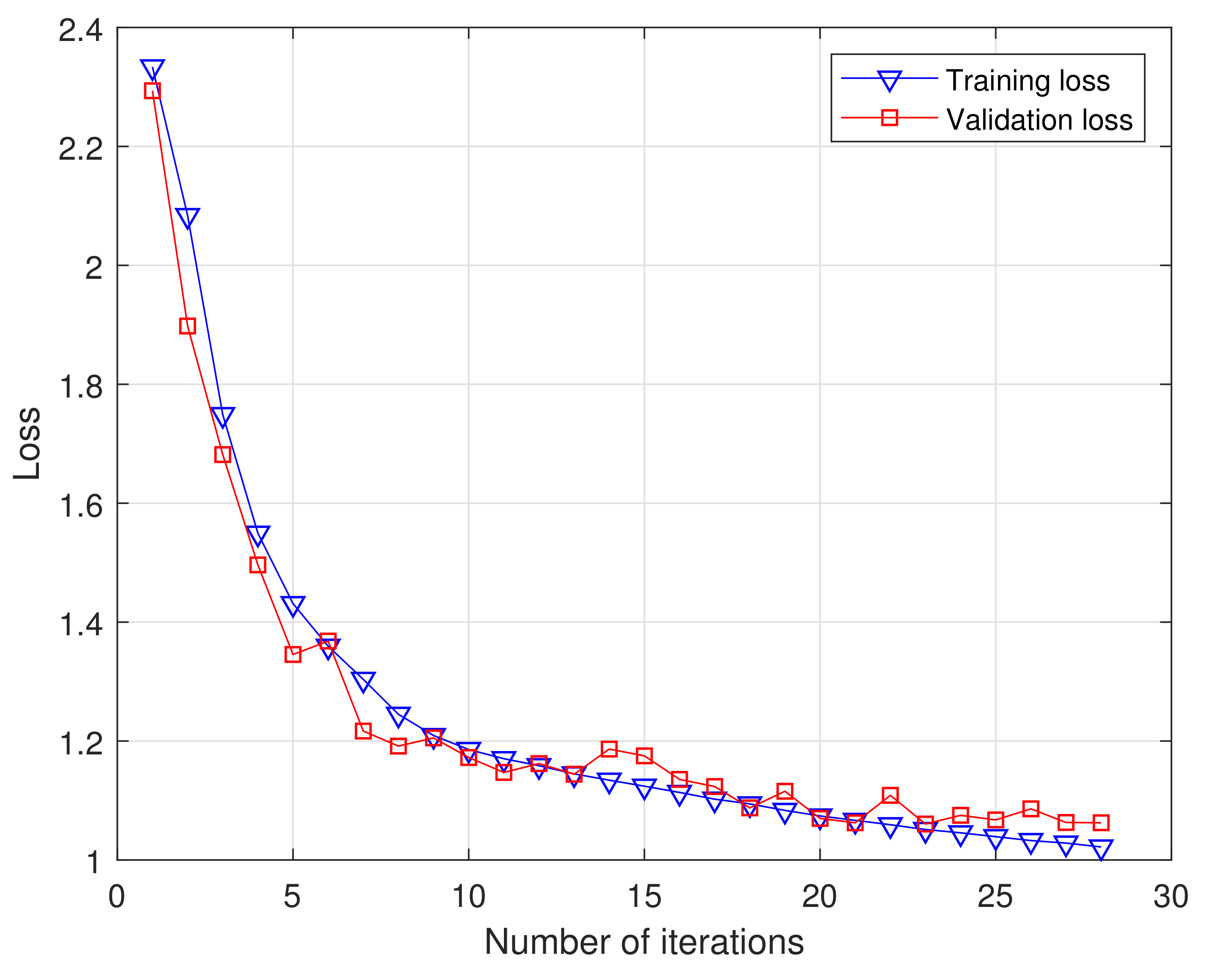
Figure 9 shows the values of the cross-entropy loss function during DCN-BiLSTM network model training and testing. As the number of iterations increases, the training and test loss values continue to decrease, indicating that the real label and the predicted label are constantly converging. When the number of iterations reaches 23, the training and testing loss values no longer decrease, and the model obtained at this time is the best.
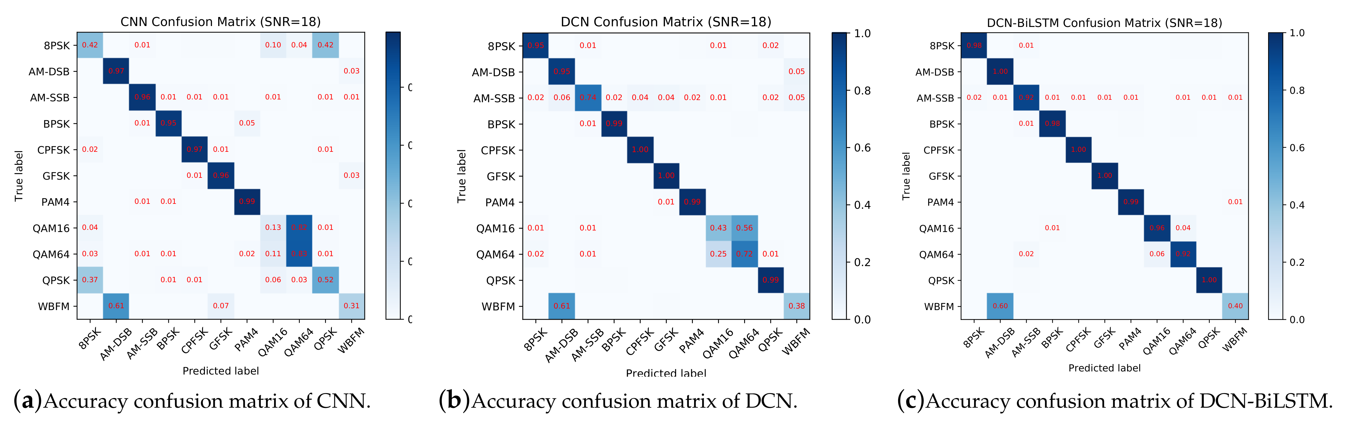
Figure 10 shows confusion matrices for the CNN, DCN and DCN-BiLSTM models when the SNR is 18 dB. According to
Figure 10a, it is difficult for the CNN to distinguish QPSK (Quadrature Phase Shift Keying) and 8PSK (8 Phase Shift Keying) because the CNN does not fully extract the phase information: the amplitudes of QPSK and 8PSK are the same and the difference between them is the phase. In addition, 16QAM (16 Quadrature Amplitude Modulation) is often misrecognized as 64QAM (64 Quadrature Amplitude Modulation) because the constellation points of 16QAM can be found in the constellation points of 64QAM.
To fully consider the phase information, we replaced the CNN with a DCN. The accuracy confusion matrix is shown in
Figure 10b. Clearly, the accuracies on the QPSK and 8PSK modulation types are much better than in
Figure 10a, and the accuracy on the 16QAM and 64QAM modulation types has improved as well. However, the accuracy on the 16QAM and 64QAM types is still not good enough for practical applications; therefore, we still need to improve their recognition accuracy.
Considering the connections among data points, we cascaded the BiLSTM after the DCN to extract the contextual information of signals. An accuracy confusion matrix for the DCN-BiLSTM is shown in
Figure 10c, showing that the recognition accuracy of 16QAM and 64QAM is greatly improved compared with the results in
Figure 10a,b. This result indicates that the BiLSTM is useful for extracting the contextual features of signals.
As shown in
Figure 10a–c, it is quite difficult to recognize wide band frequency modulation (WBFM). The reason is that the dataset uses voice signals to generate analog signals, and people’s voices have silent periods during speaking, leaving only a single carrier during the silent period. Thus, the WBFM signals can easily be misclassified as AM-DSB (amplitude modulation—double side band modulation) signals.
To fully compare the dataset recognition capabilities of the above several networks, we used an online platform that can perform statistical analysis [
30]. First, we uploaded the file representing the recognition result in csv format, as shown in
Table 3.
Table 3 shows the recognition error rate of five types of datasets. The error rates of the first four datasets correspond to the corresponding modulated signals in the fifth dataset. According to Rodríguez-Fdez et al. [
30] and the test situation in this paper, we selected Friedman [
31] as the test type to be applied. We chose Holm [
32], which is widely used, as the post-hoc with control method. At the same time, we set the significance level
to 0.05.
After experiments, the algorithm rankings obtained are shown in
Table 4. As we can see, DCN-BiLSTM has the highest ranking and its performance is better than the other seven networks. Moreover, the ranking in
Table 4 is consistent with the ranking of the recognition effect in
Figure 8, which also shows the correctness of the experiment.
Table 5 summarizes the comparison between DCN-BiLSTM and the other seven algorithms by using post-hoc with control methods. By comparing p-value with
, it can be seen that the DCN-BiLSTM network is significantly different from Inception, CNN and Resnet, indicating that the proposed network has significant progress compared with them. At the same time, there are no significant differences between DCN-BiLSTM and CLDNN, CVC, CNN-LSTM and MTL-CNN, which means that the proposed algorithm inherits the excellent performance of the four networks and can replace them in the field of modulation recognition.
4.2. Performance Comparison When Using Different Parameters for the DCN-BiLSTM Network
To obtain the best parameter configuration for the DCN-BiLSTM network, this section studies the influences of each parameter configuration on the algorithm’s performance.
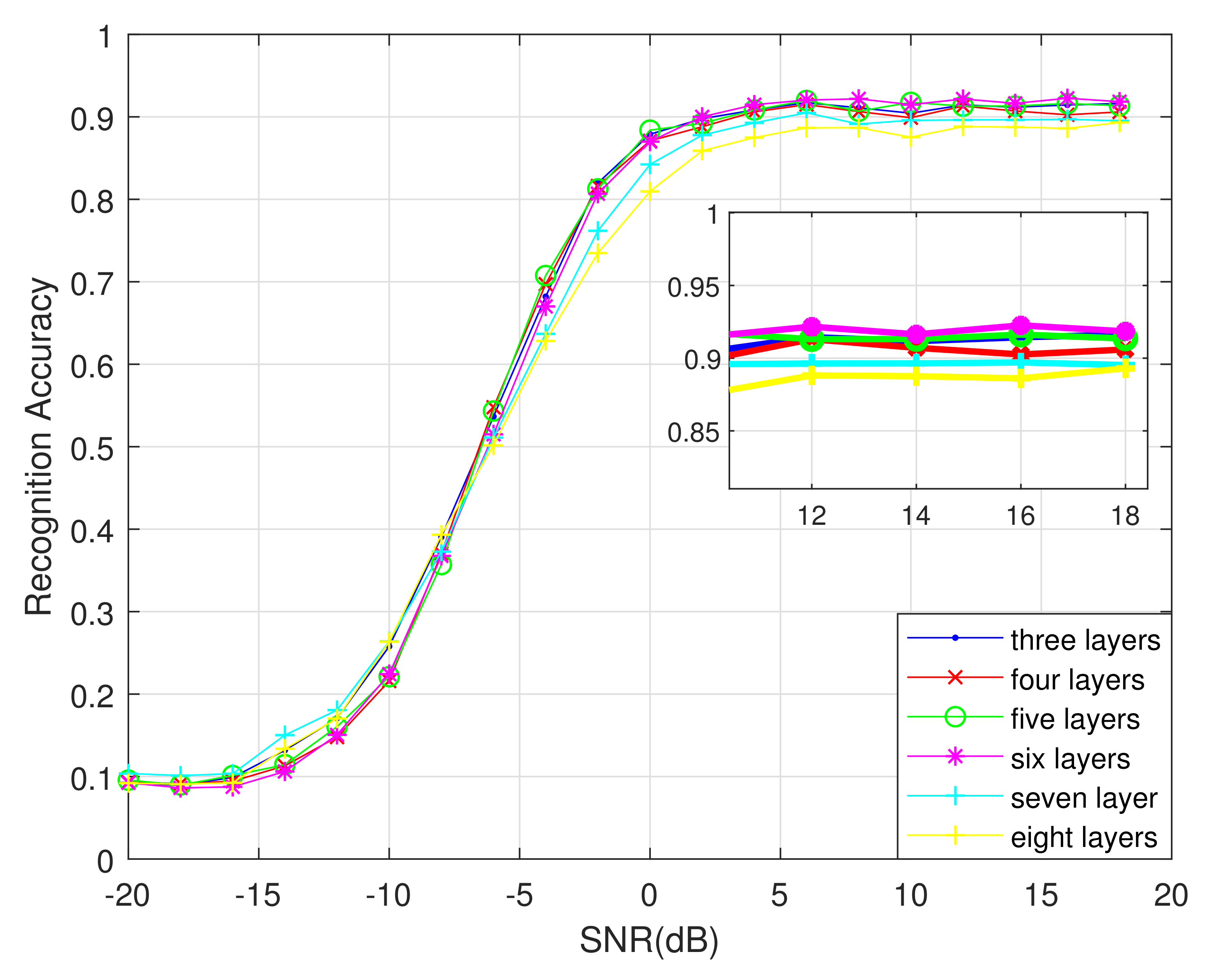
First, we change only the number of DCN layers to find the best number of DCN layers. The different recognition results are shown in
Figure 11.
As shown in
Figure 11, the overall recognition rate is the highest with six DCN layers when the SNR is greater than 2 dB. With fewer than six layers, the network’s ability to extract phase features is not strong enough. With more than six layers, the network extracts redundant features, and the recognition rate no longer improves, which wastes memory. Therefore, the best number of DCN layers for this algorithm is six.
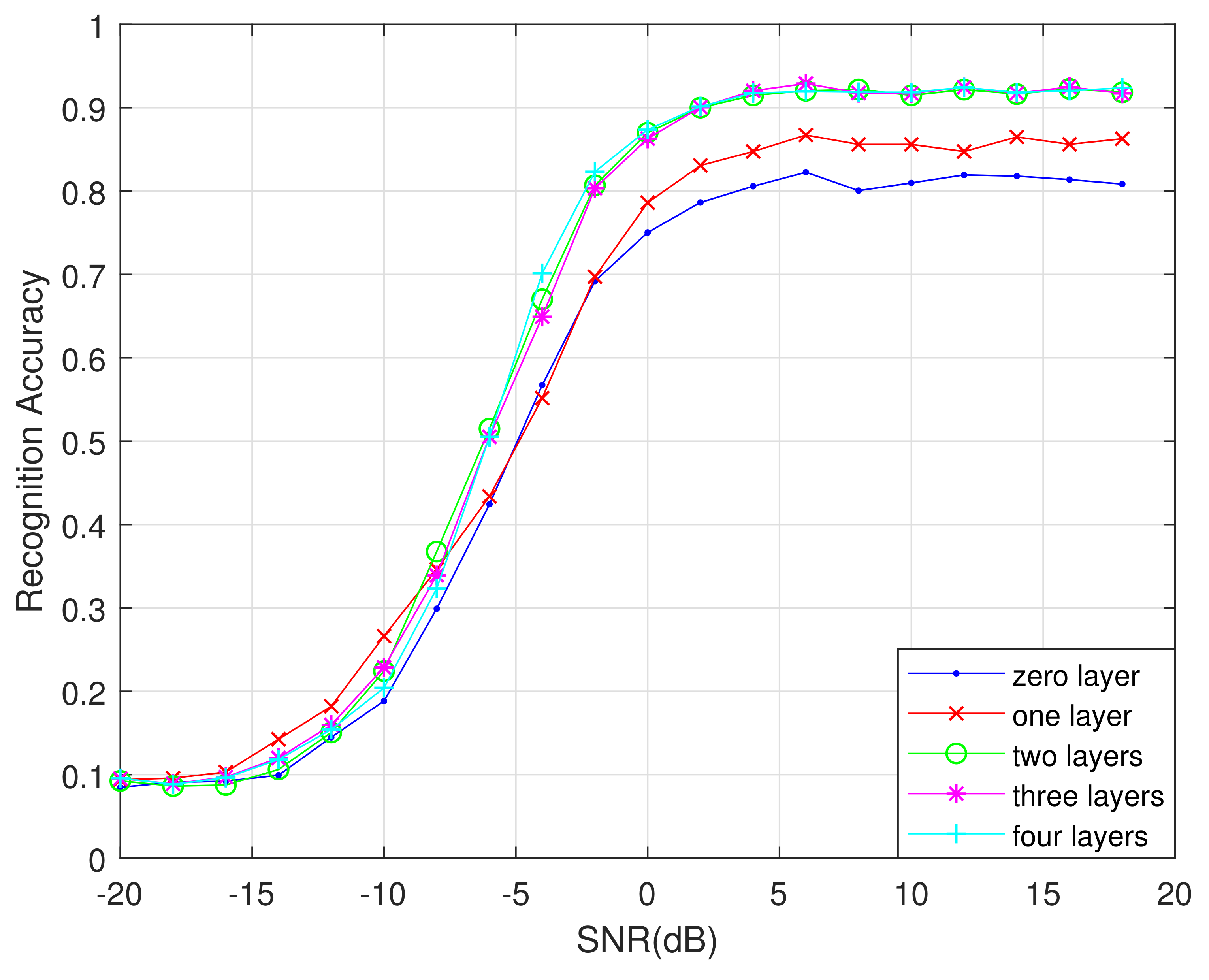
Changing the BiLSTM layer number also affects the recognition performance.
Figure 12 shows a comparison of the recognition performance under different numbers of BiLSTM layers.
With fewer than two BiLSTM layers, the algorithm’s ability to process feature information is poor. With more than two layers, while the accuracy rate is equivalent to that of a two-layer BiLSTM network, the added layers cause a speed reduction and waste memory. Therefore, it is best to set the number of BiLSTM layers to two.
Based on the previous analysis, the final DCN-BiLSTM network parameters are shown in
Table 6.
4.3. Five-Fold Cross Validation
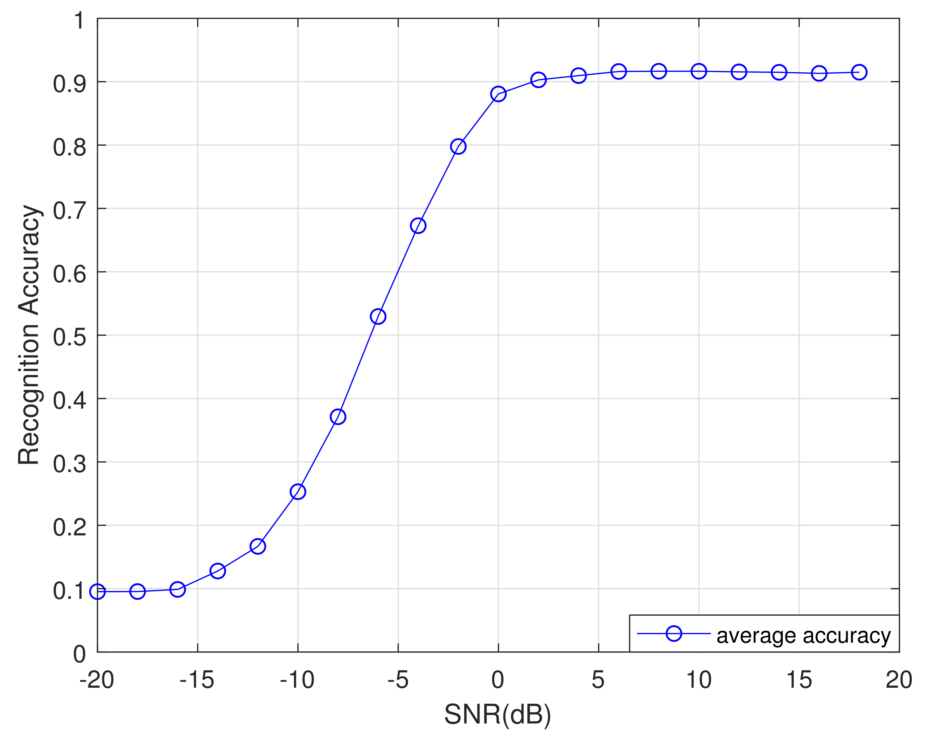
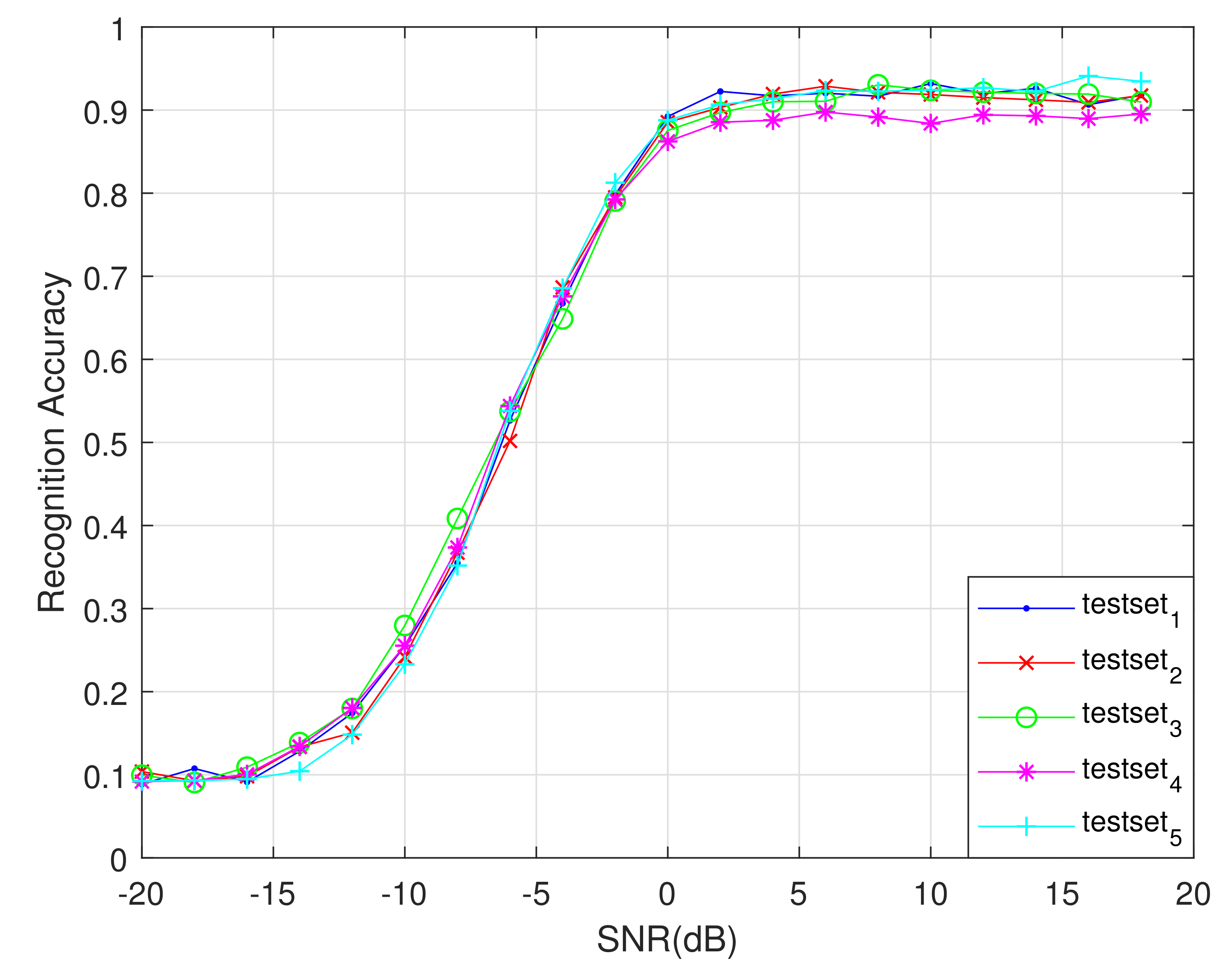
To evaluate the performance of the network proposed in this article, we used the five-fold cross-validation method to train and test the network in this part. We divide the dataset into five parts equally, and use one part as the test sets each time and the remaining four parts as the training sets. Finally we obtained five training and test results, as shown in
Figure 13. The average recognition rate curve of these five times is shown in
Figure 14. As shown in
Figure 13 and
Figure 14, when SNR is greater than 4 dB, the recognition accuracy of the proposed network is more than 90% under five trainings, covering the entire dataset, which illustrates the rationality and stability of the designed network.
5. Conclusions
In this paper, we propose a classification algorithm based on the DCN-BiLSTM network that achieves direct recognition of 11 different types of modulated signals. First, DCN layers are used to extract the phase features of the modulation signal. Then, BiLSTM layers are used to extract the contextual information and construct a bidirectional long short-term memory model for the features. Compared with previous network recognition algorithms based on CNN, Inception, Resnet, CLDNN, MTL-CNN, CVC and CNN-LSTM, the recognition accuracy of the DCN-BiLSTM network is significantly higher under high SNR. However, even when the SNR is as low as 4 dB, the recognition accuracy rate of the DCN-BiLSTM network can still reach 90%.
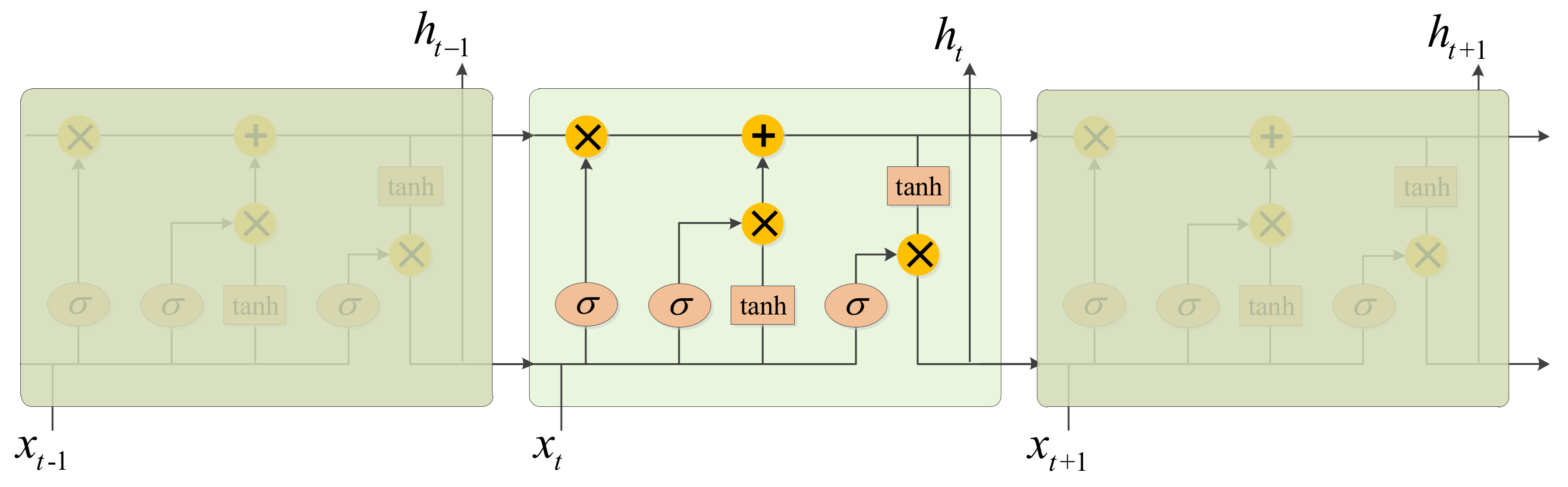
However, the DCN-BiLSTM network has a slow training speed, and the method works satisfactorily only for signals whose frequency offset and sampling frequency offset are within a certain range. In addition, the identified signal must belong to one of the 11 specified types. In future work, we plan to modify or optimize these issues. In particular, on the one hand, for the training speed issue, we can use other GPUs with stronger computing capabilities to speed up training. On the other hand, in terms of network structure, each LSTM unit in the BiLSTM layers contains three gate functions, resulting in more parameters, which is the main reason for the slow network training speed. Therefore, we can try to optimize the LSTM unit to reduce the number of parameters and increase the training speed, such as reducing or simplifying the gate function.
In addition to the phase information and contextual information mentioned in this paper, many other characteristics of modulated signals could be considered, such as time–frequency domain characteristics and constellation characteristics. In future work, we plan to use other features in combination with the DCN-BiLSTM network to improve the modulation signal identification performance.


