
Reference Frame Unification of IMU-Based Joint Angle Estimation: The Experimental Investigation and a Novel Method


Abstract
:1. Introduction
2. Related Work
3. Method and Materials
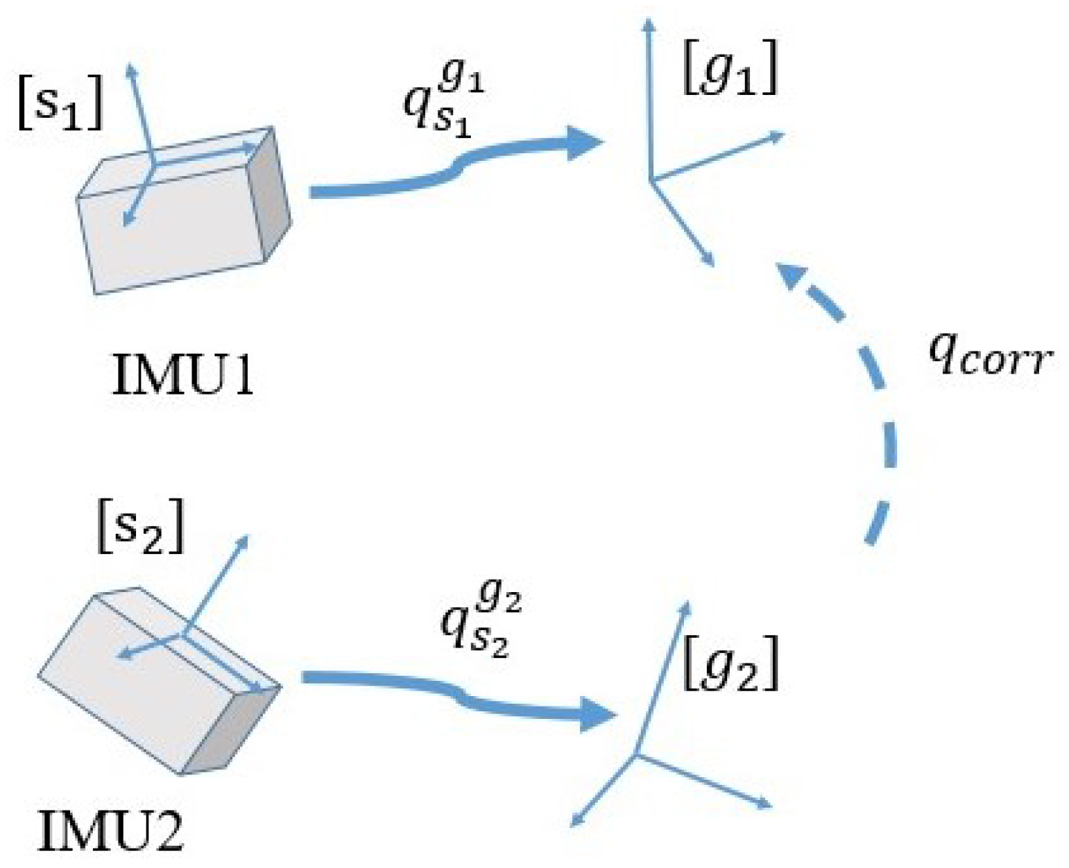
3.1. Problem Statement
3.2. Experimental Procedure
3.3. Analysis on the Characteristics of Different Reference Frames’ Deviations
3.3.1. Data Preprocessing
3.3.2. Analyzing Procedure
3.3.3. Analyzing Results
3.3.4. Findings
3.4. Reference Frame Unification with Comprehensive Metrics
3.5. Data Analysis
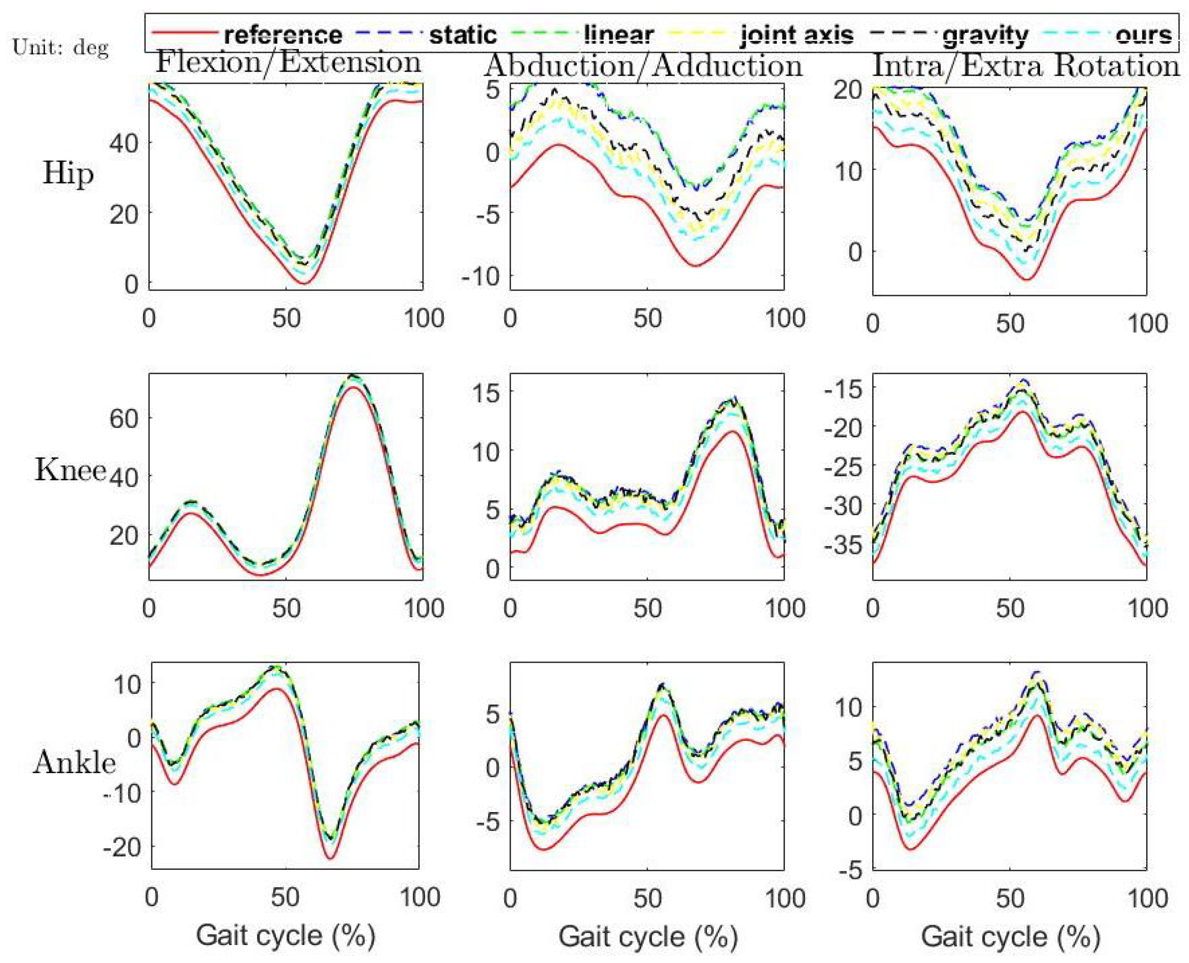
4. Results
Discussion
| Algorithm 1 RFU method with comprehensive metrics. | |
| Require: | |
| Ensure: | |
| 1: | initialize |
| 2: | while do |
| 3: | calculating the magnetometer measurement-based correction quaternion using Equation (7) |
| 4: | calculating the accelerometer measurement-based correction quaternion using Equation (6) |
| 5: | fusing and using Equation (8) |
| 6: | calculating the main axis’ projections in the reference frame using Equation (9) |
| 7: | forming the cost function as , and solving it using L-M method. |
| 8: | end while |
5. Conclusions
Author Contributions
Funding
Institutional Review Board Statement
Informed Consent Statement
Conflicts of Interest
Abbreviations
| IMU | Inertial measurement unit |
| RFU | Reference frame unification |
| DC | Drift correction |
References
- Emery, A.E. Population frequencies of inherited neuromuscular diseases—A world survey. Neuromuscul. Disord. 1991, 1, 19–29. [Google Scholar]
- Roos, E.M.; Roos, H.P.; Lohmander, L.S.; Ekdahl, C.; Beynnon, B.D. Knee Injury and Osteoarthritis Outcome Score (KOOS)—Development of a self-administered outcome measure. J. Orthop. Sports Phys. Ther. 1998, 28, 88–96. [Google Scholar] [CrossRef] [PubMed]
- Ferber, R.; Osternig, L.R.; Woollacott, M.H.; Wasielewski, N.J.; Lee, J.H. Gait mechanics in chronic ACL deficiency and subsequent repair. Clin. Biomech. 2002, 17, 274–285. [Google Scholar] [CrossRef]
- Yi, C.; Jiang, F.; Chen, Z.; Wei, B.; Guo, H.; Yin, X.; Li, F.; Yang, C. Sensor-Movement-Robust Angle Estimation for 3-DoF Lower Limb Joints Without Calibration. arXiv 2019, arXiv:1910.07240. [Google Scholar]
- Chen, Z.; Temitayo, M.; Isa, P. Pipe Flaws Detection by Using the Mindstorm Robot. Int. J. Eng. Res. Appl. 2012, 2, 569–574. [Google Scholar]
- Edwards, J.Z.; Greene, K.A.; Davis, R.S.; Kovacik, M.W.; Noe, D.A.; Askew, M.J. Measuring flexion in knee arthroplasty patients. J. Arthroplast. 2004, 19, 369–372. [Google Scholar] [CrossRef] [PubMed]
- Hatfield, G.L.; Hubley-Kozey, C.L.; Wilson, J.L.A.; Dunbar, M.J. The effect of total knee arthroplasty on knee joint kinematics and kinetics during gait. J. Arthroplast. 2011, 26, 309–318. [Google Scholar] [CrossRef]
- Ding, Y.; Panizzolo, F.A.; Siviy, C.; Malcolm, P.; Galiana, I.; Holt, K.G.; Walsh, C.J. Effect of timing of hip extension assistance during loaded walking with a soft exosuit. J. Neuroeng. Rehabil. 2016, 13, 87. [Google Scholar] [CrossRef] [PubMed] [Green Version]
- Ding, Y.; Galiana, I.; Siviy, C.; Panizzolo, F.A.; Walsh, C. IMU-based iterative control for hip extension assistance with a soft exosuit. In Proceedings of the 2016 IEEE International Conference on Robotics and Automation (ICRA), Stockholm, Sweden, 16–21 May 2016; pp. 3501–3508. [Google Scholar]
- Qu, X.; Yeo, J.C. Effects of load carriage and fatigue on gait characteristics. J. Biomech. 2011, 44, 1259–1263. [Google Scholar] [CrossRef]
- Birrell, S.A.; Haslam, R.A. The effect of load distribution within military load carriage systems on the kinetics of human gait. Appl. Ergon. 2010, 41, 585–590. [Google Scholar] [CrossRef] [PubMed]
- Tzu-wei, P.H.; Kuo, A.D. Mechanics and energetics of load carriage during human walking. J. Exp. Biol. 2014, 217, 605–613. [Google Scholar]
- Fasel, B.; Spörri, J.; Schütz, P.; Lorenzetti, S.; Aminian, K. Validation of functional calibration and strap-down joint drift correction for computing 3D joint angles of knee, hip, and trunk in alpine skiing. PLoS ONE 2017, 12, e0181446. [Google Scholar] [CrossRef]
- Sainsbury, D. Serge Van Sint Jan, Color Atlas of Skeletal Landmark Definitions, Churchill Livingstone/Elsevier (2007) ISBN 9-78-0443-10315-5 181. Physiotherapy 2009, 95, 234–235. [Google Scholar] [CrossRef]
- Leardini, A.; Biagi, F.; Merlo, A.; Belvedere, C.; Benedetti, M.G. Multi-segment trunk kinematics during locomotion and elementary exercises. Clin. Biomech. 2011, 26, 562–571. [Google Scholar] [CrossRef]
- Lu, T.W.; O’connor, J. Bone position estimation from skin marker co-ordinates using global optimisation with joint constraints. J. Biomech. 1999, 32, 129–134. [Google Scholar] [CrossRef]
- Leardini, A.; Belvedere, C.; Nardini, F.; Sancisi, N.; Conconi, M.; Parenti-Castelli, V. Kinematic models of lower limb joints for musculo-skeletal modelling and optimization in gait analysis. J. Biomech. 2017, 62, 77–86. [Google Scholar] [CrossRef]
- Kadaba, M.P.; Ramakrishnan, H.; Wootten, M. Measurement of lower extremity kinematics during level walking. J. Orthop. Res. 1990, 8, 383–392. [Google Scholar] [CrossRef] [PubMed]
- Sabatini, A.M. Estimating Three-Dimensional Orientation of Human Body Parts by Inertial/Magnetic Sensing. Sensors 2011, 11, 1489–1525. [Google Scholar] [CrossRef] [Green Version]
- Ligorio, G.; Sabatini, A.M. A Novel Kalman Filter for Human Motion Tracking with an Inertial-Based Dynamic Inclinometer. IEEE Trans. Biomed. Eng. 2015, 62, 2033–2043. [Google Scholar] [CrossRef]
- Roetenberg, D.; Baten, C.T.M.; Veltink, P.H. Estimating Body Segment Orientation by Applying Inertial and Magnetic Sensing Near Ferromagnetic Materials. IEEE Trans. Neural Syst. Rehabil. Eng. 2007, 15, 469–471. [Google Scholar] [CrossRef] [Green Version]
- Yi, C.; Ma, J.; Guo, H.; Han, J.; Gao, H.; Jiang, F.; Yang, C. Estimating three-dimensional body orientation based on an improved complementary filter for human motion tracking. Sensors 2018, 18, 3765. [Google Scholar] [CrossRef] [Green Version]
- Brennan, A.; Zhang, J.; Deluzio, K.; Li, Q. Quantification of inertial sensor-based 3D joint angle measurement accuracy using an instrumented gimbal. Gait Posture 2011, 34, 320–323. [Google Scholar] [CrossRef]
- Adamowicz, L.; Gurchiek, R.D.; Ferri, J.; Ursiny, A.T.; Fiorentino, N.; McGinnis, R.S. Validation of Novel Relative Orientation and Inertial Sensor-to-Segment Alignment Algorithms for Estimating 3D Hip Joint Angles. Sensors 2019, 19, 5143. [Google Scholar] [CrossRef] [PubMed] [Green Version]
- Palermo, E.; Rossi, S.; Marini, F.; Patanè, F.; Cappa, P. Experimental evaluation of accuracy and repeatability of a novel body-to-sensor calibration procedure for inertial sensor-based gait analysis. Measurement 2014, 52, 145–155. [Google Scholar] [CrossRef]
- Hagemeister, N.; Parent, G.; Van de Putte, M.; St-Onge, N.; Duval, N.; de Guise, J. A reproducible method for studying three-dimensional knee kinematics. J. Biomech. 2005, 38, 1926–1931. [Google Scholar] [CrossRef]
- Seel, T.; Raisch, J.; Schauer, T. IMU-based joint angle measurement for gait analysis. Sensors 2014, 14, 6891–6909. [Google Scholar] [CrossRef] [PubMed] [Green Version]
- Favre, J.; Jolles, B.; Aissaoui, R.; Aminian, K. Ambulatory measurement of 3D knee joint angle. J. Biomech. 2008, 41, 1029–1035. [Google Scholar] [CrossRef] [PubMed]
- Vitali, R.V.; Cain, S.M.; McGinnis, R.S.; Zaferiou, A.M.; Ojeda, L.V.; Davidson, S.P.; Perkins, N.C. Method for estimating three-dimensional knee rotations using two inertial measurement units: Validation with a coordinate measurement machine. Sensors 2017, 17, 1970. [Google Scholar] [CrossRef] [Green Version]
- Laidig, D.; Schauer, T.; Seel, T. Exploiting kinematic constraints to compensate magnetic disturbances when calculating joint angles of approximate hinge joints from orientation estimates of inertial sensors. In Proceedings of the 2017 International Conference on Rehabilitation Robotics (ICORR), London, UK, 17–20 July 2017; pp. 971–976. [Google Scholar]
- Seel, T.; Ruppin, S. Eliminating the effect of magnetic disturbances on the inclination estimates of inertial sensors. IFAC-PapersOnLine 2017, 50, 8798–8803. [Google Scholar] [CrossRef]
- Fan, B.; Li, Q.; Wang, C.; Liu, T. An adaptive orientation estimation method for magnetic and inertial sensors in the presence of magnetic disturbances. Sensors 2017, 17, 1161. [Google Scholar] [CrossRef]
- Yadav, N.; Bleakley, C. Accurate orientation estimation using AHRS under conditions of magnetic distortion. Sensors 2014, 14, 20008–20024. [Google Scholar] [CrossRef] [PubMed] [Green Version]
- Crabolu, M.; Pani, D.; Raffo, L.; Cereatti, A. Estimation of the center of rotation using wearable magneto-inertial sensors. J. Biomech. 2016, 49, 3928–3933. [Google Scholar] [CrossRef] [PubMed]


| Static | Linear | Joint Axis | Gravity | Ours | ||
|---|---|---|---|---|---|---|
| Ankle | flexion/extension | 4.3 ± 0.4 | 3.8 ± 0.5 | 3.6 ± 0.8 | 3.9 ± 0.8 | 2.7 ± 0.6 |
| abduction/adduction | 2.7 ± 0.5 | 2.3 ± 0.7 | 2.0 ± 0.4 | 2.1 ± 0.7 | 1.4 ± 0.6 | |
| intra/extra rotation | 2.8 ± 0.4 | 2.6 ± 0.7 | 2.4 ± 0.7 | 2.4 ± 0.8 | 1.1 ± 0.6 | |
| Knee | flexion/extension | 4.0 ± 0.5 | 4.1 ± 0.4 | 3.5 ± 0.8 | 3.9 ± 0.8 | 2.6 ± 0.4 |
| abduction/adduction | 2.8 ± 0.5 | 2.6 ± 0.4 | 2.2 ± 0.8 | 2.5 ± 0.8 | 1.5 ± 0.4 | |
| intra/extra rotation | 2.7 ± 0.5 | 2.7 ± 0.4 | 2.4 ± 0.8 | 2.8 ± 0.8 | 1.3 ± 0.4 | |
| Hip | flexion/extension | 7.2 ± 0.4 | 7.0 ± 0.6 | 5.1 ± 0.3 | 5.5 ± 0.5 | 2.8 ± 0.3 |
| abduction/adduction | 6.3 ± 0.5 | 6.5 ± 0.6 | 3.2 ± 0.6 | 4.1 ± 0.7 | 2.1 ± 0.5 | |
| intra/extra rotation | 6.8 ± 0.6 | 6.6 ± 0.5 | 2.3 ± 0.5 | 3.9 ± 0.4 | 2.0 ± 0.3 | |
| Static | Linear | Joint Axis | Gravity | Ours |
|---|---|---|---|---|
| 2.56 | 2.37 | 3.74 | 4.37 | 2.89 |
Publisher’s Note: MDPI stays neutral with regard to jurisdictional claims in published maps and institutional affiliations. |
© 2021 by the authors. Licensee MDPI, Basel, Switzerland. This article is an open access article distributed under the terms and conditions of the Creative Commons Attribution (CC BY) license (http://creativecommons.org/licenses/by/4.0/).
Share and Cite
Yi, C.; Jiang, F.; Yang, C.; Chen, Z.; Ding, Z.; Liu, J. Reference Frame Unification of IMU-Based Joint Angle Estimation: The Experimental Investigation and a Novel Method. Sensors 2021, 21, 1813. https://doi.org/10.3390/s21051813
Yi C, Jiang F, Yang C, Chen Z, Ding Z, Liu J. Reference Frame Unification of IMU-Based Joint Angle Estimation: The Experimental Investigation and a Novel Method. Sensors. 2021; 21(5):1813. https://doi.org/10.3390/s21051813
Chicago/Turabian StyleYi, Chunzhi, Feng Jiang, Chifu Yang, Zhiyuan Chen, Zhen Ding, and Jie Liu. 2021. "Reference Frame Unification of IMU-Based Joint Angle Estimation: The Experimental Investigation and a Novel Method" Sensors 21, no. 5: 1813. https://doi.org/10.3390/s21051813