4.2. Experimental Evaluation of TUM RGB-D Datasets
The TUM RGB-D datasets are offered by the Computer Vision Group of the Technical University of Munich and were recorded in different environments with a Microsoft Kinect RGB-D camera. Dataset Resolution: a unique motion capture system records 640 × 480, frame rate: 30 (FPS), the ground-truth is recorded by a special motion capture system.
- 4.
Fr1_xyz uses a device that is an RGB-D camera (Microsoft Kinect RGB-D camera), and the acquired include both RGB image and depth image. The dataset is chosen because the images all become blurred when the camera moves rapidly, accompanied by repeated up-down/left-right movements, which brings some challenges to the robustness of the motion.
- 5.
Fr2_desk uses the same equipment and records data with loop, this dataset is mainly to check the loop and the accuracy of localization.
We select two datasets for testing (fr1_xyz/fr2_desk) as shown in
Figure 6.
We chose SVO, PL-SVO, and improved PL-SVO (the improved method in this article) for testing during the experiment:
SVO: Open sourced by ETH Zurich, the open-source SVO has simplified for some reason.
PL-SVO: Line features are added based on SVO, which improved accuracy and robustness in a low-texture environment.
Improved PL-SVO: Optimizing information theory (JS divergence) is added based on PL-SVO.
As shown in
Figure 7 each row represents the trajectory of the same system over time/number of frame, each column represents the trajectory of different systems over the same time/number of frames.
Figure 7 shows the trajectories of three systems in the TUM RGB-D Dataset fr2_desk. The number of frames in this dataset is around 3000. The primary process is to take pictures around the desktop with a camera to verify the accuracy of the algorithm.
As seen in the first column, SVO initialization is completed successfully, but during the running process, rapid movement and motion blurring cause the SVO location to fail. As the dataset runs, the relocalization of SVO is turned on, and the current camera pose is retrieved by matching with the previous keyframes and projection of map points after the motion tracking is lost, resulting in discontinuous trajectories. PL-SVO works well but also has interruptions with large gaps at F = 900 frames. IT-SVO is superior to PL-SVO in that the overall trajectory is smoother and at F = 2500 frames the interval is smaller. Due to more keyframes are extracted, the current camera pose is restored quickly by the relocalization module.
The advantage of SVO is its speed. We tested it on airborne platform devices (DJI matrice100, NVIDIA XAVIER) and it reached 55 FPS, while on PC it reached 70 FPS. It is well known that the most feared scenes of camera motion are estimated to be pure rotation, changes in light intensity, motion blur, etc., so it is easy to lose in places where the trajectory changes sharply. Since the estimation and optimization of the poses all rely on grayscale matching, this leads to the lack of robustness of the system to illumination, while point features are selected, and the features in the scene are not sufficiently described.
In the complex environment, a large number of point features are extracted while having a simple keyframe selection strategy, resulting in unrepresentative keyframes, which can easily be terminated in the re-localization due to inadequate keyframe information.
Figure 8 shows the trajectories of three systems in the TUM RGB-D dataset fr1_xyz. Because of the partial censoring of the SVO open-source algorithm, the running results of fr1_xyz are difficult to verify. When F = 50 frames, SVO has not finished initialization, so the camera does not generate a motion trajectory. PL-SVO and IT-SVO completed the initialization at the same number of frames and successfully generated the trajectories, mainly reflected in the better relocalization and depth update module. However, with the continuation of the dataset, PL-SVO has discontinuities in the left and right corners, due to the outliers generated by the fast movement. Based on
KL divergence, it is more challenging for SVO and KL-SVO to extract sufficient depth information from the disordered outliers. When F = 600 frames, there are also discontinuities at the up and down motion corners, while IT-SVO completes the location accurately and produce a smooth trajectory. During the algorithm, SVO has a poor localization performance for a hand-held camera (for the top view of UAV), PL-SVO can generate smooth trajectories under horizontal and vertical motion, its performance is poor at the corner, and IT-SVO completes tracking better.
We modified the SVO to improve its robustness and accuracy by adding line features to the point features. For efficiency we convert the line features to edge features, i.e., segment the line features.
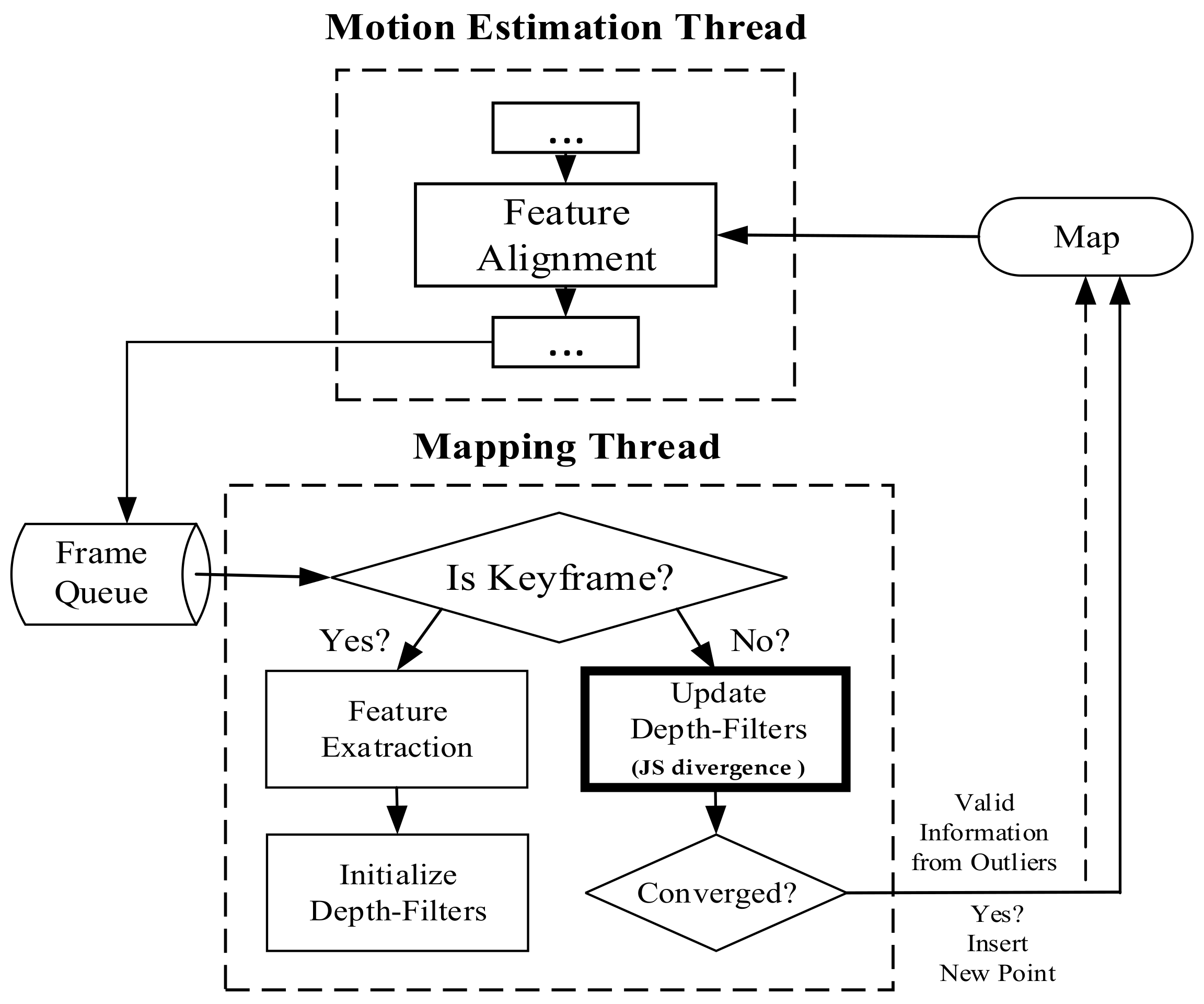
First, the mapping thread provides the initial depth based on the tracking thread. Then, the build thread calculates the exact depth and feeds it back to the tracking thread to achieve the pose estimation. In this process, the JS divergence is used to optimize the mapping thread, and the mean-Gaussian filter is used to suppress the outlier when solving for map points.
We compare the performance of the improved SVO with state-of-the-art systems, i.e., SVO, PL-SVO.
Table 1 shows the comparative results of RMSE for ATE. Trans, and Rot representing RMSE of relative pose error (RPE) of the translation and rotation, respectively, where “-” means tracking failure. The smallest indicate the best accuracy (the trajectory lengths of fr1_xyz and fr2_desk are 7.122 and 12.6 m, respectively).
As can be seen from
Table 1, SVO can barely complete the location, so it is set to “-”, which represents the data is invalid-in fr1_xyz, fast steering, up-and-down movement lead to low robustness of the PL-SVO and underestimation of the scene scale. Similiarly in fr2_desk, the rapid movement of the camera results in two relocalizations. In contrast, IT-SVO has a lower RMSE of ATE and RMSE of RPE, which improves the robustness and accuracy. The number of key frames is selected by three systems as shown in
Figure 9.
In
Table 1. xyz/right: fr2_desk the
x-axis represents the system type, and the
y-axis represents the number of keyframes. In terms of the number of keyframes, it can be seen that compared with the state-of-the-art, PL-SVO, the improved SVO has a small improvement. As described in
Section 4.1 Experimental Description, we know that there are many map points in the keyframes. On the contrary, the depth of the map points is obtained through the mapping thread, and both coexist with a linear relationship between the number of keyframes and the amount of information.
Due to the rapid movement of the camera in fr1_xyz, SVO initialization and relocalization start almost simultaneously. PL-SVO and IT-SVO require initialization of point-and-line features, which are slower than SVO in the initialization phase. The comparison of initialization time is illustrated in
Figure 10.
From the comparison of initialization time in
Figure 10, it can be seen that SVO has a long initialization time for the dataset fr1_xyz and a short initialization time for fr2_desk, which needs to be explained in third aspects for this problem:
First, for fr1_xyz, we can see that the scene is single and partly white desktop and black computer. As SVO only extracts point features, although a large number of fast corners can be extracted, it is difficult to obtain map points with effective depth information, so it is necessary to perform multiple translations to achieve the initialization of the system.
Second, for fr2_desk, we can see that the scene is complex and colorful, the SVO can easily accomplish the initialization, and in contrast to PL-SVO/IT-SVO which need to extract point/line features at the same time, the initialization can be finished quickly under complex textures.
Third, PL-SVO/IT-SVO both have the same front-end (tracking thread) and have the ability of stable feature extraction. The difference in initialization time between them is mainly reflected in the back-end (mapping thread) feedback for generating valid map points. Because of the rapid movement of the camera in fr1_xyz, SVO initialization and relocalization start almost simultaneously. PL-SVO and IT-SVO require the initialization of point-and-line features. SVO runs poorly in both datasets and impossible to complete, so relocalization time is ignored and represented by “-“. The relocalization time (s) are listed in
Table 2.
4.3. Experimental Evaluation of EuRoC Datasets
We evaluate our method by using the EuRoC MAV visual-inertia datasets. The data is collected on the MAV, including a binocular camera (used to capture stereo images, FPS: 20), an IMU measurement (200 Hz) and an image resolution of 752 × 480. This experiment only uses the image sequence collected by the left camera. We select two datasets for testing (MH01/MH02). The dataset is shown in
Figure 11.
- (1)
The content of MH01/MH02 are recorded by the UAV during flight, and the data include image from the binocular as well as the IMU. The EuRoC datasets are divided into three levels: easy/medium/high, the content of image include rotation, movement, turning, etc., and is mainly used to test the coupling algorithms of IMU and image in restricted mobile devices.
- (2)
The high level exists fast movements and is mainly suitable for testing algorithms of IMU+Camera, including DSO/ORB-SLAM2 are unable to complete that level currently, so we chose two datasets for easy and medium levels.
We chose the datasets collected in a factory in this experiment and chose the same SVO/PL-SVO/IT-SVO for testing. The results are shown in
Figure 12.
In
Figure 12 and
Figure 13, each row represents the trajectory of the same system over time/number of frames. Each column represents the trajectory of different systems over the same time/number of frames. There are three main reasons why SVO trajectory failure occur in quite smooth regions:
First, SVO is a monocular visual odometery with no closed-loop detection, which means that relocalization will not be possible when the position difference is significant.
Second, SVO compares the current frame with the previous frame to obtain a rough estimate of the pose, therefore requires the previous frame to be sufficiently accurate. If the previous frame is lost due to occlusion, blurring, etc., then the current frame will also get an incorrect result (we need a solution to effectively suppress the outlier), resulting in a poor comparison with the map, so the system will easily stop and the trajectory will have a large interruption.
Third, the smooth linear motion causes the SVO to store a considerable number of seed points, but the depth filter converges much slower than the seed point selection speed, which leads to depth mis-estimation and serious underestimation, and intuitively generates a interruption in the running.
Figure 12 shows the trajectories of three systems in the EuRoC Datasets MH01. The number of frames in this dataset is about 3700. The main content of this dataset is visual localization and navigation in a factory using IMU and camera on MAV. F = 700 is the initialization of the MAV by lifting and rotating. In the first row, due to the fast movement and insufficient point feature extraction, the initialization of SVO is low, there are more localization failures, and scale uncertainties occur during the straight-line operation. Inter-frame drift occurs when F = 3500, and the algorithm basically fails. PL-SVO and IT-SVO complete initialization, but localization fails when their running in a straight line. IT-SVO fails only on a small straight line, but it achieves tracking soon after relocalization. IT-SVO has better performance than SVO and PL-SVO in running datasets. The detailed error analysis is shown in
Table 3.
In
Figure 14, the SVO still has fewer keyframes, most of which are due to the instability of the system and the complex variation of the environmental characteristics. Compared with PL-SVO, the improved SVO has a little improvement. As described experimentally, the selection of keyframes brings some robustness to the system.
In
Figure 15, the initialization time is longer for the three systems because the initial state of the EuRoC Datasets requires initializing the camera and IMU. The initialization of the IMU requires static initialization, which has a longer initialization time than the TUM RGB-D Datasets.
The overall MH01/MH02 initialization time is higher than fr1_xyz/fr2_desk because the former requires to initialize the IMU at the same time, so the device must be stationary, while the vision-based algorithm only needs to have some translation to complete the initialization, so the initialization time is longer than the latter.
As shown in
Table 4, compared with the first two systems, the improved SVO has a better relocalization function, mainly in terms of the shorter time. The relocalization time (s) are listed in
Table 4.
Finally, the experiments were performed multiple times while the FPS of the processed image was used to indicate the speed. As shown in
Table 5.
The processing speed on PC is higher than the onboard processor of the mobile device, but for a full-HD camera the processing speed will be slower, because in the tracking thread we only follow the third level of the pyramid, and the depth of scene will be complemented by the mapping thread.
4.4. Experiment and Comparison of Generalization Ability of Visual Odometry
We tested on the whole TUM RGB-D datasets, totaling twenty-three groups, and performed the corresponding experimental results and trajectory analysis. Then we choose the well-known ORB-SLAM2 for experimental comparison and select eight groups of experiments in which the proposed algorithm outperforms ORBSLAM2. Finally, the comparison video will be put to the link in the paper.
In the TUM RGB-D datasets, four groups of the robot SLAM category: (fr2_pioneer_360/fr2_pioneer_slam/fr2_pioneer_slam2/fr2_pioneer_slam3), all the comparison algorithms mentioned in this paper cannot be completed (including ORB-SLAM2). Meanwhile, we show the experimental screenshots of the datasets as well as the trajectories. In
Figure 16, eight groups of datasets and trajectories are illustrated.
fr1/fr2: The data collected by different cameras, and some datasets that should be clarified.
fr1_rpy: This dataset represents the rotation of the camera in space to verify the rotational invariance and motion robustness of the proposed algorithm, while ORB-SLAM2 is difficult to initialize, which leads to operational failure.
fr1_floor: The main scene of this dataset is the ground (containing inhomogeneous light), where IT-SVO can achieve localization. In contrast, ORB-SLAM2 has difficulty in extracting feature points in repetitive low-texture environments and cannot complete the initialization, which leads to localization failure.
There are also several unfinished datasets containing white ground, white boxes and open field, where SVO, PL-SVO, ORB-SLAM2 and IT-SVO all fail to achieve localization (fr1_360/fr2_large_with_loop/fr3_nostructure_notexture_near_with_loop). Finally, related to that provide seven groups of demonstrations of IT-SVO outperforming ORB-SLAM2 in the
Supplementary Materials, and the code will be open source in the future.
In
Figure 17 and
Figure 18, we compare the number of keyframe selections and the time of initialization, as well as the detailed error analysis given in
Table 6.
As shown in
Figure 17, SVO does not work in the majority of environments, and in
Table 6, IT-SVO outperforms PL-SVO in terms of accuracy and robustness. where a lower ATE means that the trajectory is closer to the ground-truth.
At the same time, we also tested the algorithm on the EuRoC datasets, in which due to the the difficulty level, ORB-SLAM2 that only takes the localization mode and the algorithm proposed in this paper cannot be completed, mainly because of the fast moving of the UAV. As shown in
Figure 19, we tested on the additional datasets V1_01_easy, V2_01_easy, mav03_medium and V2_02_medium except for the difficulty level. The trajectory is generated from keyframes and connected under the temporal sequence. Also, it is a criterion to evaluate the accuracy of the algorithm.
Figure 20 and
Figure 21 show the comparison of the number of keyframes and the initialization time, respectively, followed by the corresponding error analysis in
Table 7.
Finally, we performed experiments with a total of twenty-three groups and related to that seven groups of demonstrations of IT-SVO outperforming ORB-SLAM2 in the
Supplementary Materials.


