
Error Prediction of Air Quality at Monitoring Stations Using Random Forest in a Total Error Framework


Abstract
:1. Introduction
- (i)
- Buying fixed air quality monitoring stations that respect DQOs.
- (ii)
- Field operation and quality control according to procedures following standards developed by the European Committee for Standardization (CEN).
- (i)
- Acquiring the measurements from the data logger into an environmental database hosted on its servers.
- (ii)
- Helping cities respecting protocols for the maintenance and the data quality control.
- (iii)
- Checking the entire Norwegian AQ observation and sending quarterly reports to the Norwegian Environmental Agency as part of preparing for the national AQ reporting to the European Commission.
1.1. Outliers and Their Detection Methods
1.2. Importance of Weighting the Quality of an Observation
1.3. AQ Prediction and Its Predictive Uncertainty
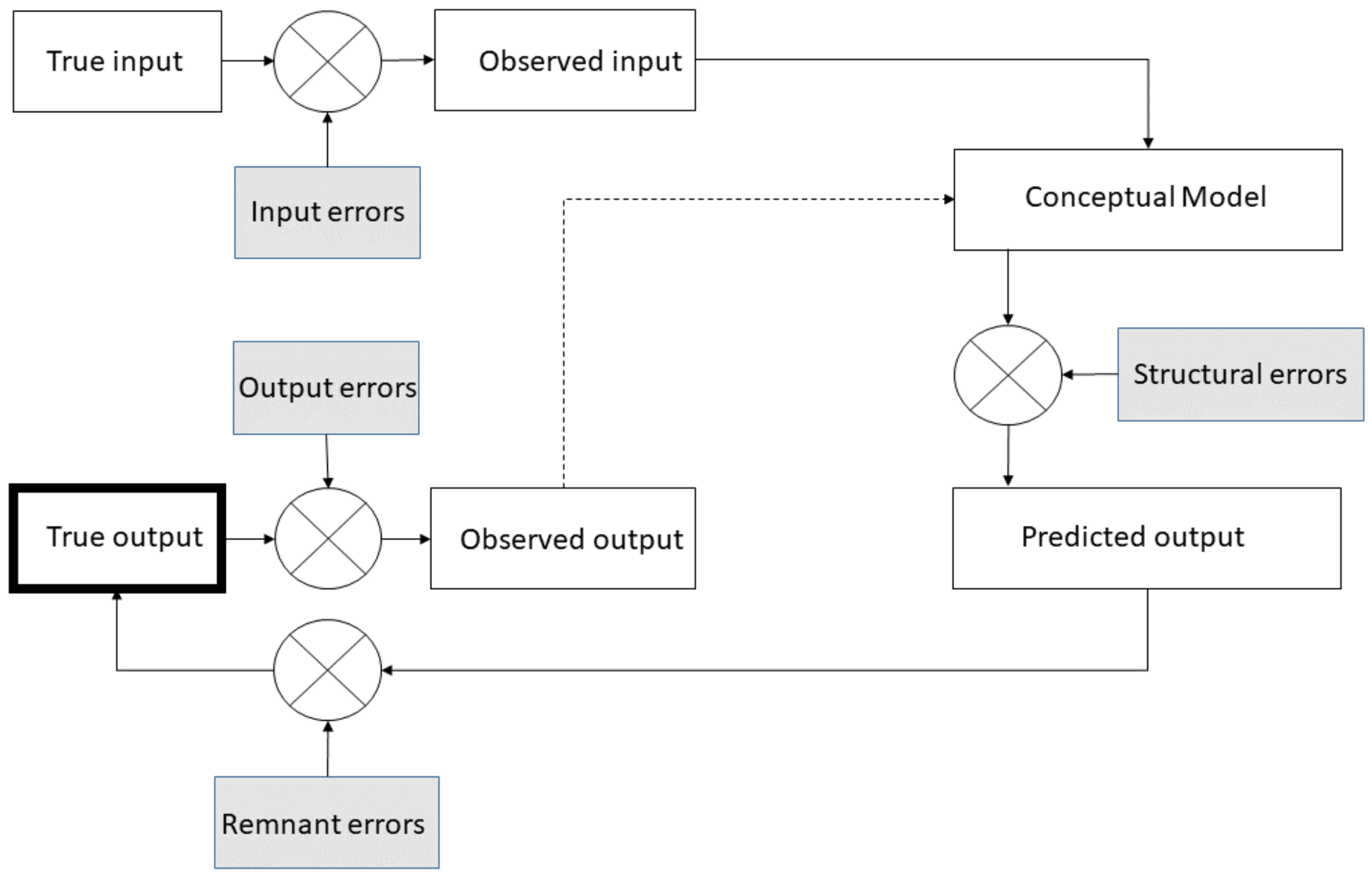
1.4. Total Error Framework
1.5. Objectives and Contributions
1.6. Outline of the Paper
2. Materials and Methods
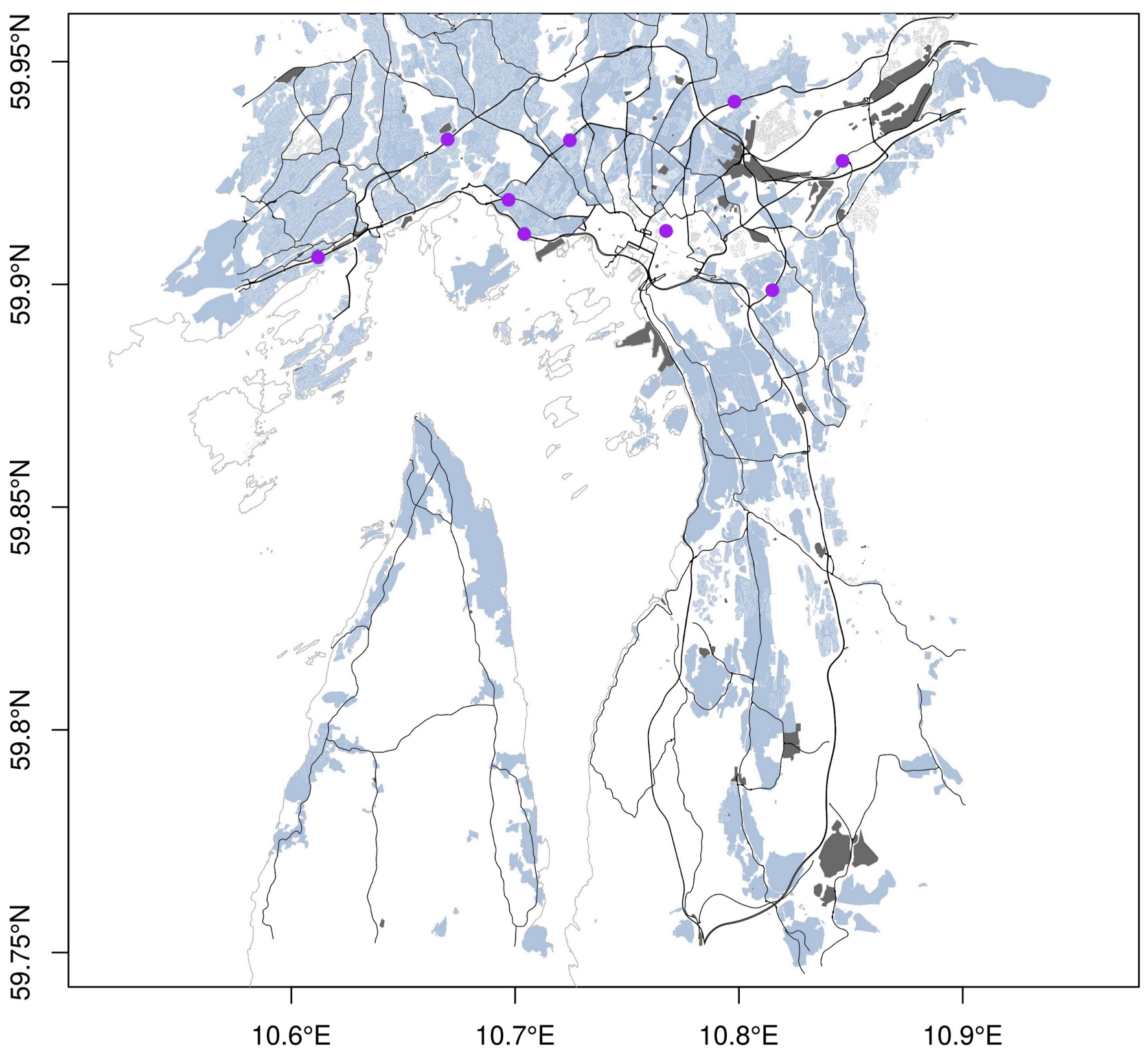
2.1. Air Quality Monitoring Stations in the Metropolitan Region of Oslo, Norway
2.1.1. Instrumentation of AQ Station Measuring Concentration
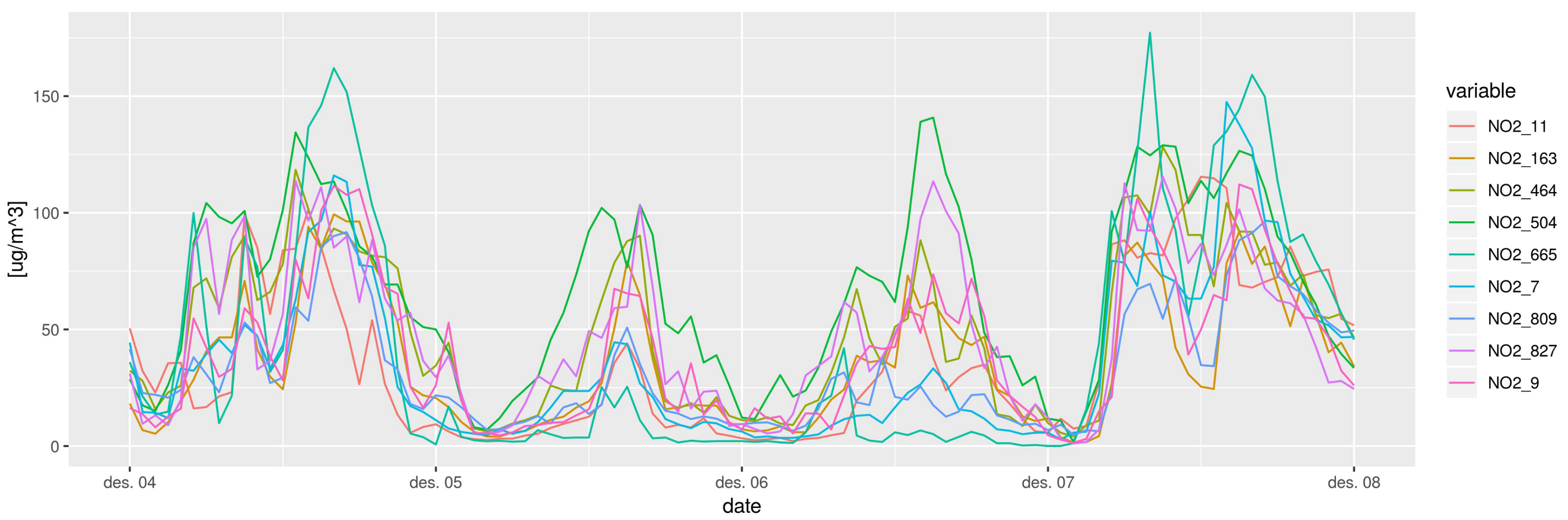
2.1.2. Hourly Concentration Dataset
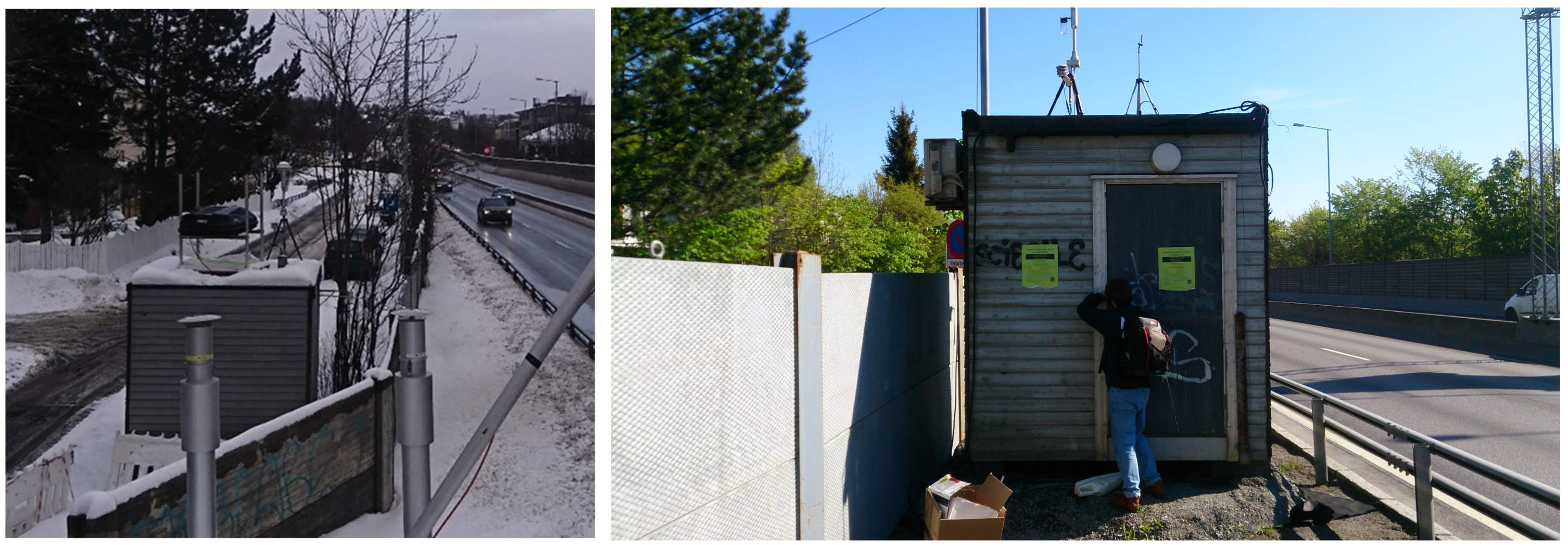
2.1.3. Road Work at Smestad between 2015 and 2016
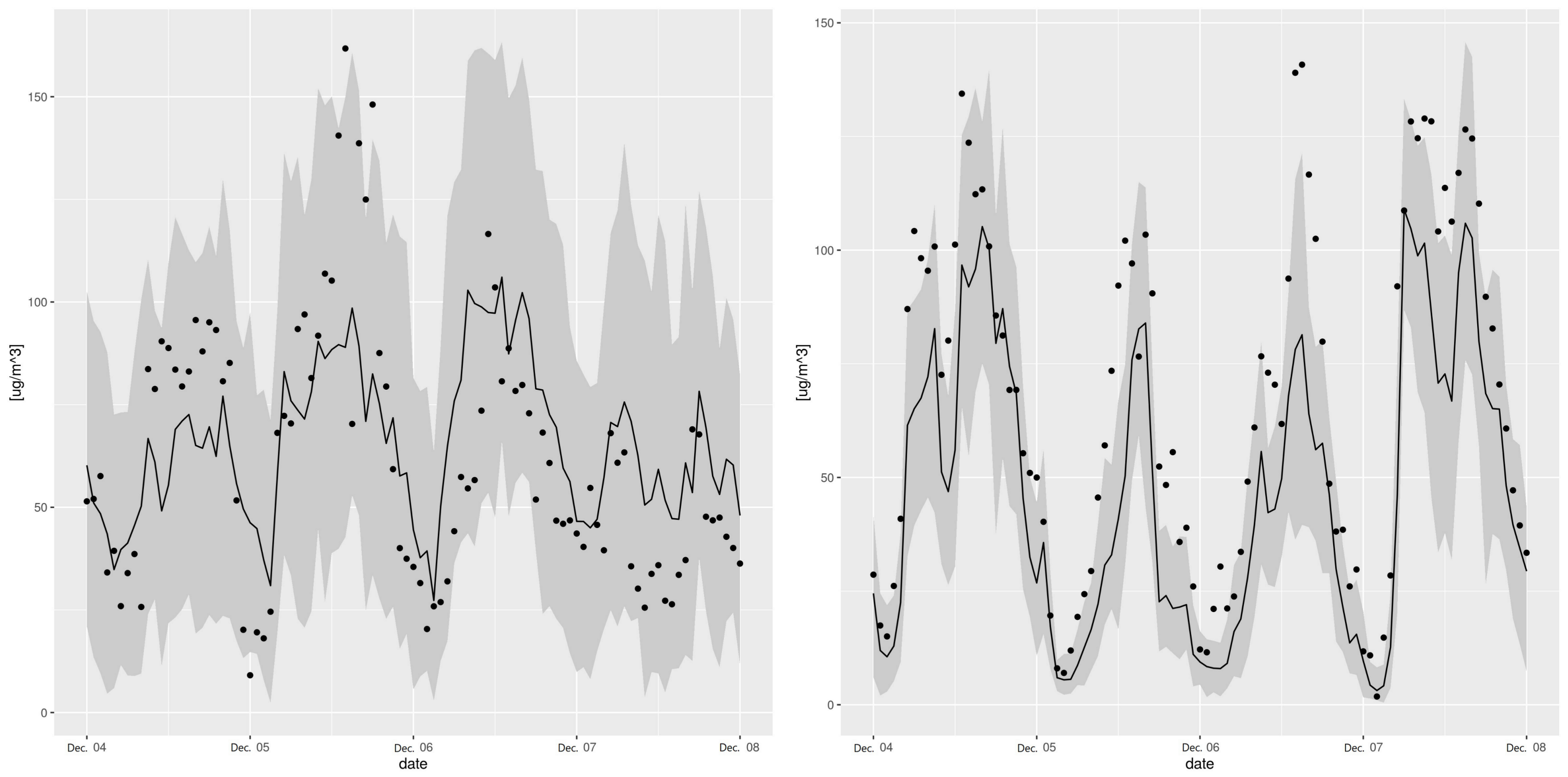
2.2. Air Quality Prediction Using RFreg in a Total Error Framework
2.2.1. Theoretical Approach
2.2.2. Approach by Eaamm 2010
2.2.3. Approach by Wager 2014
2.2.4. Approach by Lu 2019
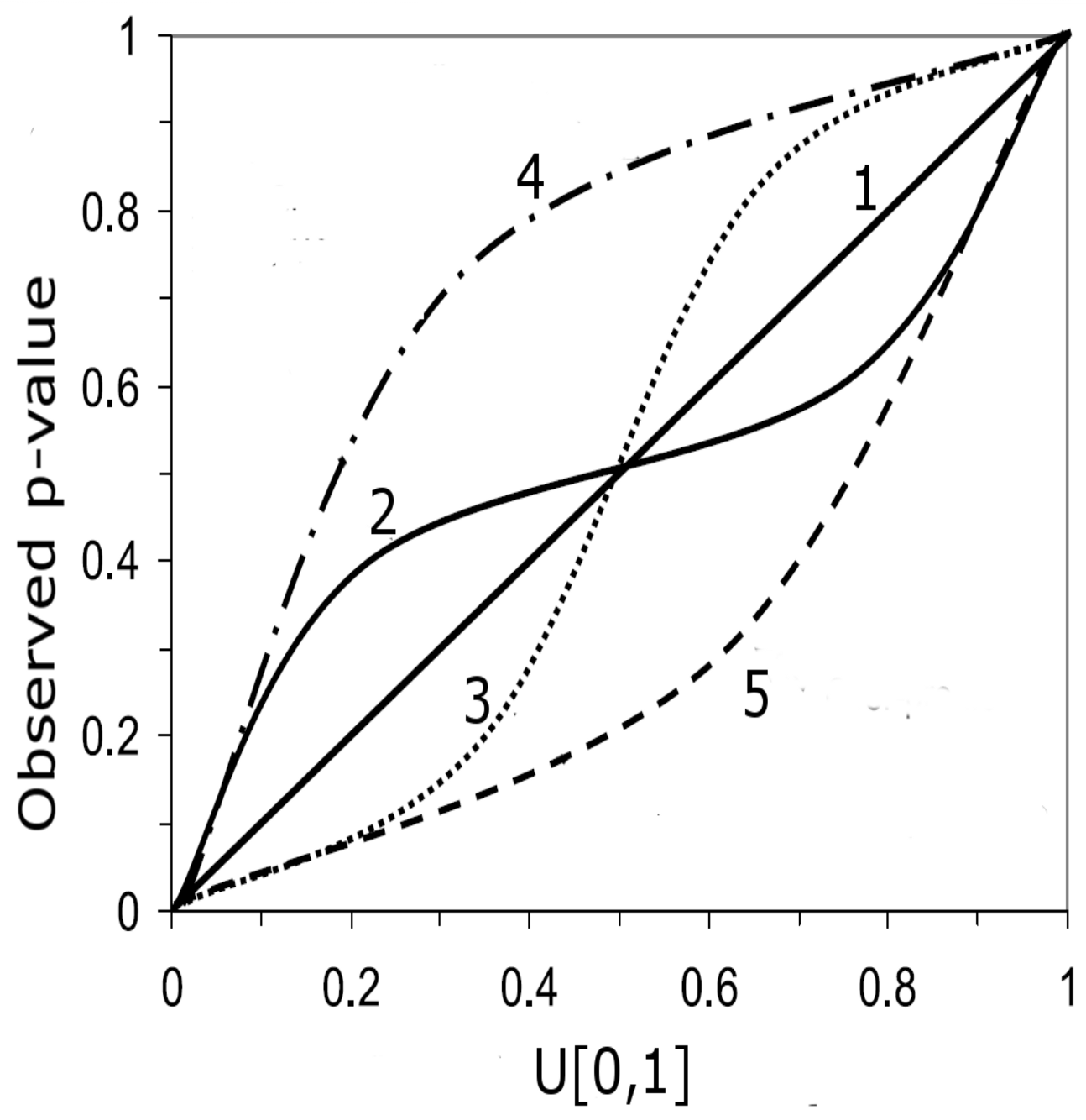
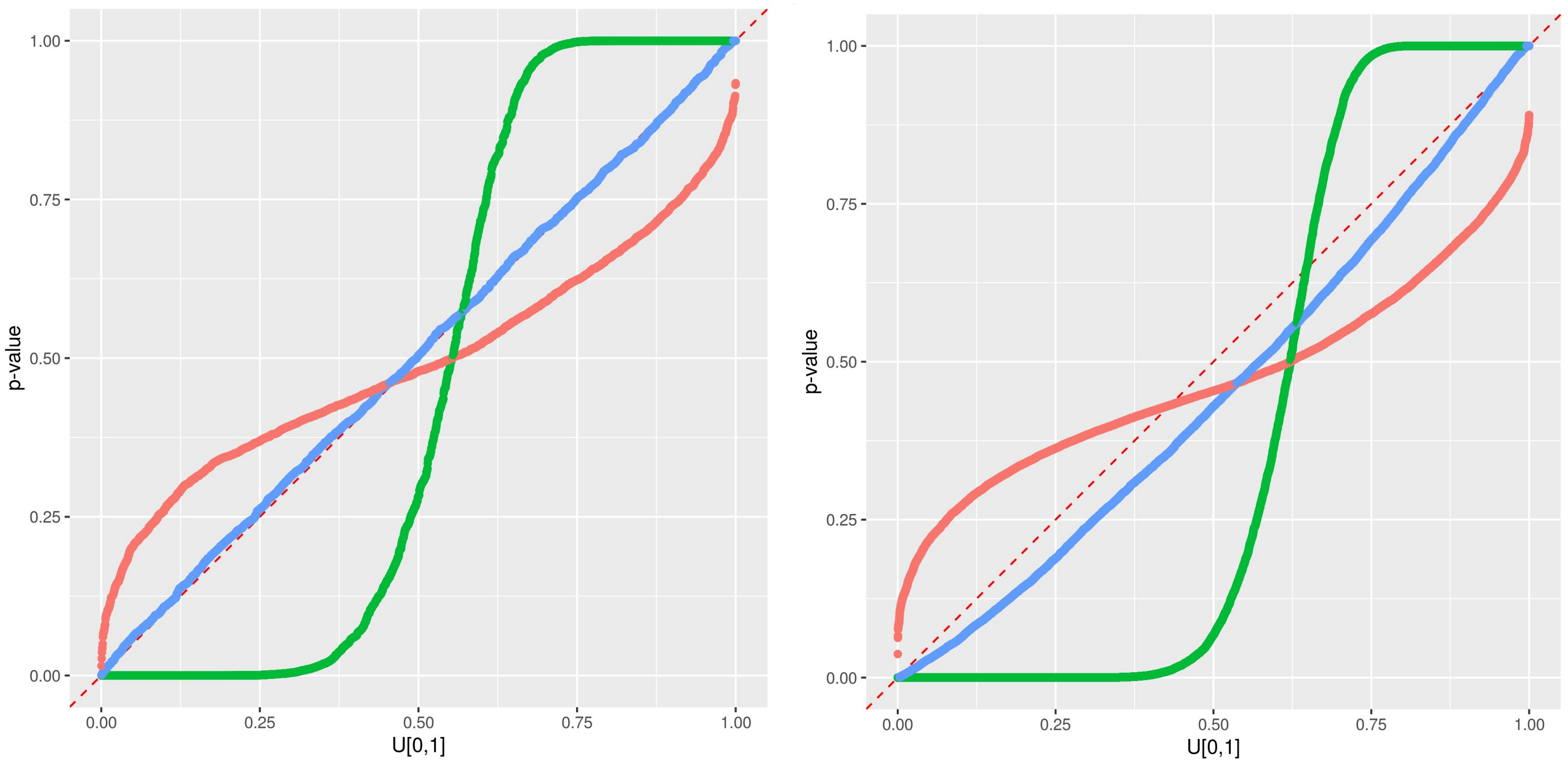
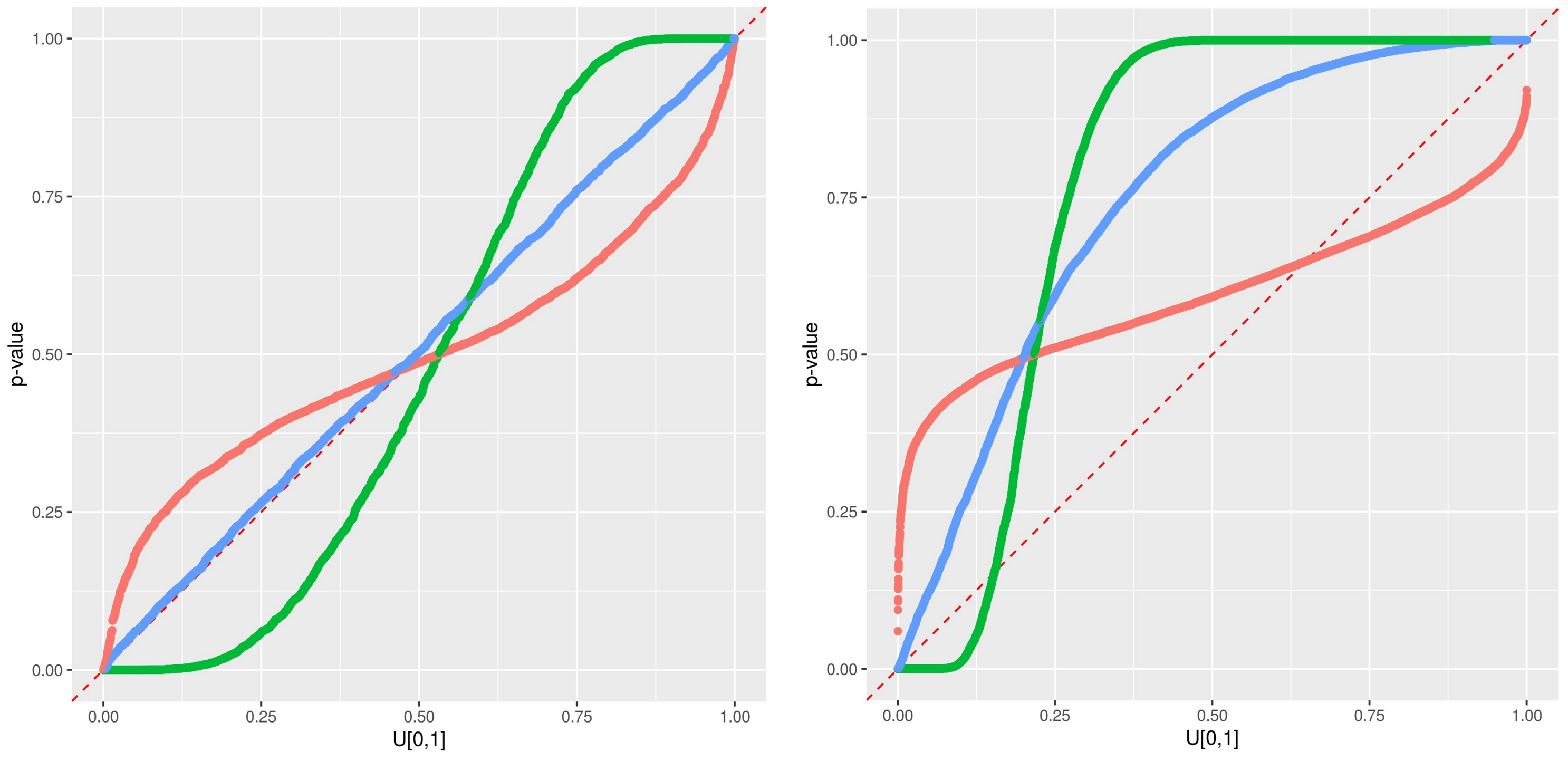
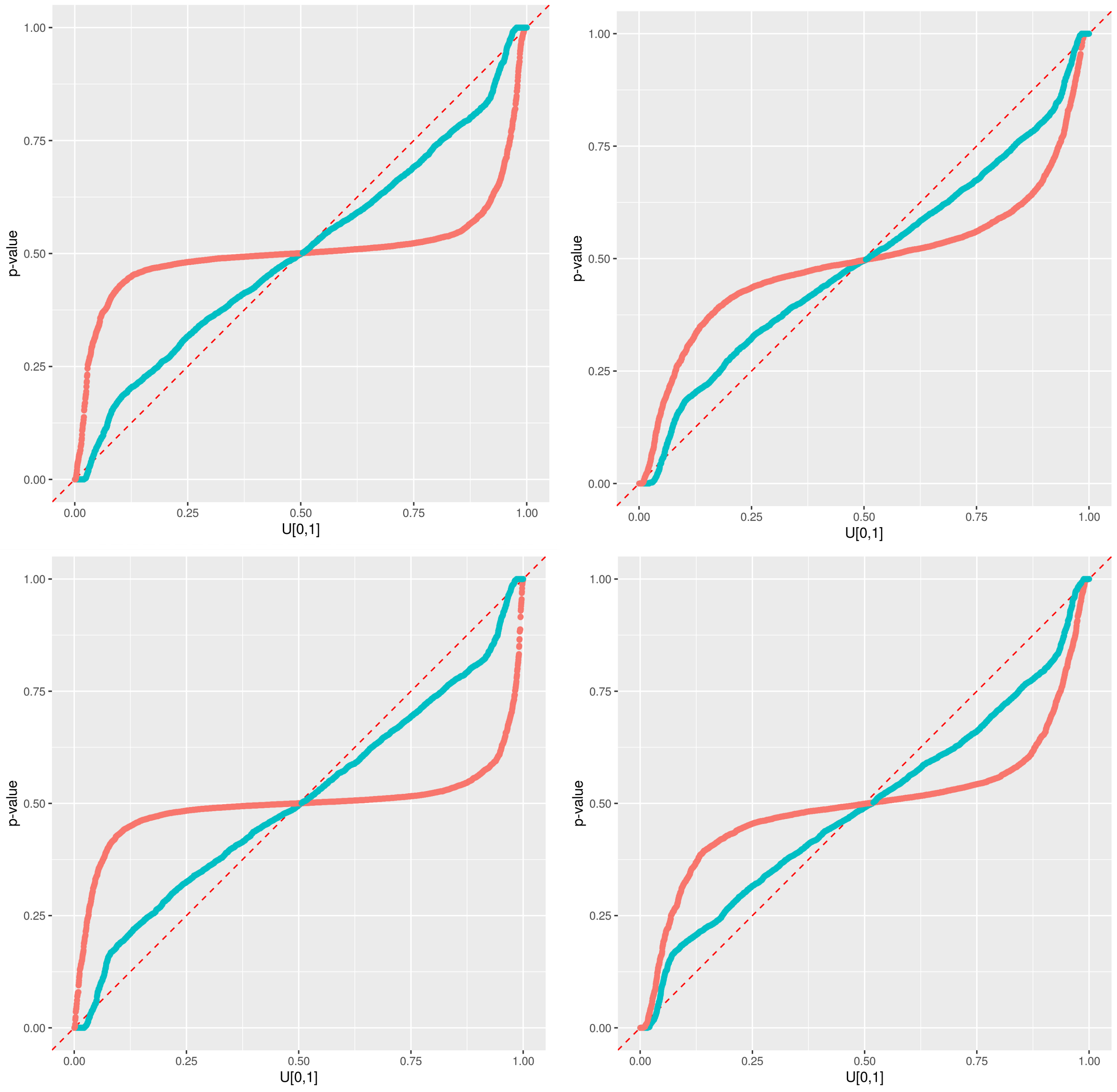
2.3. Predictive qq-Plot: Diagnostic to p-Values
- –
- Case 1: If all points fall on the 1:1 line, the predicted distribution agrees perfectly with the observations.
- –
- Case 2: the window of the predicted error is overestimated.
- –
- Case 3: the window of the predicted error is underestimated.
- –
- Case 4: the prediction model systematically under-predict the observed data.
- –
- Case 5: the prediction model systematically over-predict the observed data.
- –
- Case 6: When an observed p-value is 1.0 or 0.0, the corresponding observed data lies outside the predicted range, implying that the error prediction is significantly underestimated.
2.4. Experimentation Plan
2.4.1. Comparison of the Three Approaches
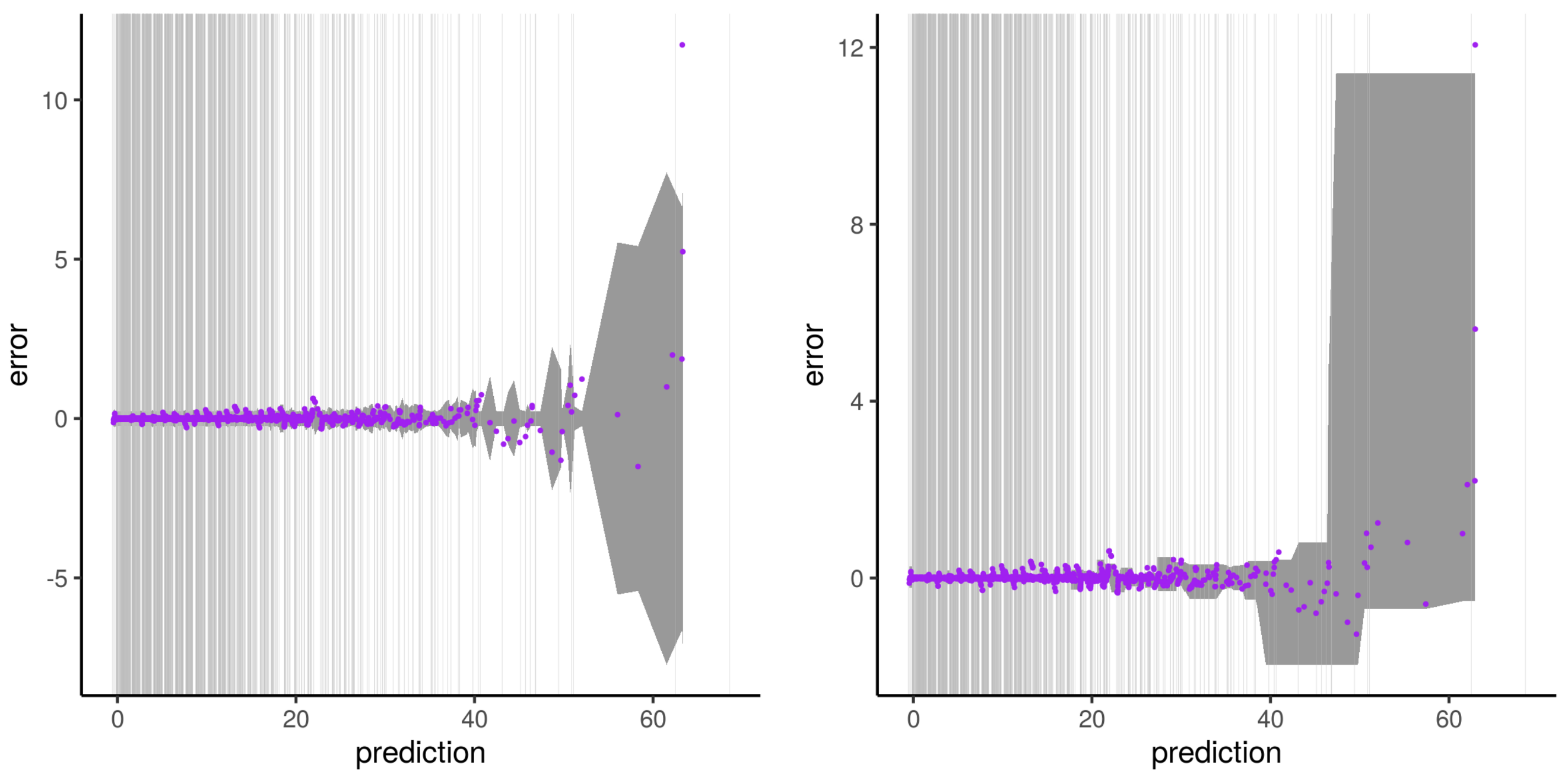
2.4.2. Quantifying the Structural Modeling Error of RFreg with Synthetic Datasets
3. Results
3.1. Metrics of AQ Prediction Based on RFreg
3.2. Comparison of the Three Approaches
3.3. Structural Modeling of RFreg
3.4. Discussion
4. Conclusions
Author Contributions
Funding
Data Availability Statement
Acknowledgments
Conflicts of Interest
References
- Liu, H.; Schneider, P.; Haugen, R.; Vogt, M. Performance Assessment of a Low-Cost PM2.5 Sensor for a near Four-Month Period in Oslo, Norway. Atmosphere 2019, 10, 41. [Google Scholar] [CrossRef] [Green Version]
- Spinelle, L.; Gerboles, M.; Villani, M.G.; Aleixandre, M.; Bonavitacola, F. Field calibration of a cluster of low-cost available sensors for air quality monitoring. Part A: Ozone and nitrogen dioxide. Sens. Actuators B Chem. 2015, 215, 249–257. [Google Scholar] [CrossRef]
- Hamer, P.; Walker, S.; Sousa-Santos, G.; Vogt, M.; Vo-Thanh, D.; Lopez-Aparicio, S.; Ramacher, M.; Karl, M. The urban dispersion model EPISODE. Part 1: A Eulerian and subgrid-scale air quality model and its application in Nordic winter conditions. Geosci. Model Dev. Discuss. 2019, 2019. [Google Scholar] [CrossRef] [Green Version]
- Shishegaran, A.; Saeedi, M.; Kumar, A.; Ghiasinejad, H. Prediction of air quality in Tehran by developing the nonlinear ensemble model. J. Clean. Prod. 2020, 259, 120825. [Google Scholar] [CrossRef]
- Schneider, P.; Castell, N.; Vogt, M.; Dauge, F.R.; Lahoz, W.A.; Bartonova, A. Mapping urban air quality in near real-time using observations from low-cost sensors and model information. Environ. Int. 2017, 106, 234–247. [Google Scholar] [CrossRef]
- Lahoz, W.A.; Khatattov, B.; Ménard, R. Data Assimilation: Making Sense of Observations; Springer: Berlin/Heidelberg, Germany, 2010. [Google Scholar] [CrossRef]
- Inness, A.; Ades, M.; Agustí-Panareda, A.; Barré, J.; Benedictow, A.; Blechschmidt, A.M.; Dominguez, J.J.; Engelen, R.; Eskes, H.; Flemming, J.; et al. The CAMS reanalysis of atmospheric composition. Atmos. Chem. Phys. 2019, 19, 3515–3556. [Google Scholar] [CrossRef] [Green Version]
- Directive 2008/50/EC of the European Parliament and of the Council of 21 May 2008 on ambient air quality and cleaner air for Europe. Off. J. Eur. Union 2008, 152, 1–44. [CrossRef]
- Yao, Y.; Sharma, A.; Golubchik, L.; Govindan, R. Online anomaly detection for sensor systems: A simple and efficient approach. Perform. Eval. 2010, 67, 1059–1075. [Google Scholar] [CrossRef]
- Cheng, H.; Tan, P.N.; Potter, C.; Klooster, S. Detection and Characterization of Anomalies in Multivariate Time Series. In Proceedings of the 2009 SIAM International Conference on Data Mining, Sparks, NV, USA, 30 April–2 May 2009; pp. 413–424. [Google Scholar] [CrossRef] [Green Version]
- Goldstein, M.; Uchida, S. A Comparative Evaluation of Unsupervised Anomaly Detection Algorithms for Multivariate Data. PLoS ONE 2016, 11, e0152173. [Google Scholar] [CrossRef] [Green Version]
- Bosman, H.; Iacca, G.; Tejada, A.; Wörtche, H.; Liotta, A. Ensembles of incremental learners to detect anomalies in ad hoc sensor networks. Ad Hoc Netw. 2015, 35, 14–36. [Google Scholar] [CrossRef]
- Wu, H.J.; Tang, X.; Wang, Z.F.; Wu, L.; Lu, M.M.; Wei, L.F.; Zhu, J. Probabilistic Automatic Outlier Detection for Surface Air Quality Measurements from the China National Environmental Monitoring Network. Adv. Atmos. Sci. 2018, 35, 1522–1532. [Google Scholar] [CrossRef]
- Gerboles, M.; Reuter, H.I. Estimation of the Measurement Uncertainty of Ambient Air Pollution Datasets Using Geostatistical Analysis; Technical Report 59441, EUR 24475 EN; Publications Office of the European Union: Luxembourg, 2010. [Google Scholar] [CrossRef]
- Li, J.; Pedrycz, W.; Jamal, I. Multivariate time series anomaly detection: A framework of Hidden Markov Models. Appl. Soft Comput. 2017, 60, 229–240. [Google Scholar] [CrossRef]
- Li, X.; Peng, L.; Hu, Y.; Shao, J.; Chi, T. Deep learning architecture for air quality predictions. Environ. Sci. Pollut. Res. 2016, 23, 22408–22417. [Google Scholar] [CrossRef]
- Li, X.; Peng, L.; Yao, X.; Cui, S.; Hu, Y.; You, C.; Chi, T. Long short-term memory neural network for air pollutant concentration predictions: Method development and evaluation. Environ. Pollut. 2017, 231, 997–1004. [Google Scholar] [CrossRef]
- Zhao, J.; Deng, F.; Cai, Y.; Chen, J. Long short-term memory-Fully connected (LSTM-FC) neural network for PM2.5 concentration prediction. Chemosphere 2019, 220, 486–492. [Google Scholar] [CrossRef]
- Huang, C.J.; Kuo, P.H. A deep cnn-lstm model for particulate matter (PM2.5) forecasting in smart cities. Sensors 2018, 18, 2220. [Google Scholar] [CrossRef] [Green Version]
- Qi, Y.; Li, Q.; Karimian, H.; Liu, D. A hybrid model for spatiotemporal forecasting of PM2.5 based on graph convolutional neural network and long short-term memory. Sci. Total Environ. 2019, 664, 1–10. [Google Scholar] [CrossRef] [PubMed]
- Blundell, C.; Cornebise, J.; Kavukcuoglu, K.; Wierstra, D. Weight uncertainty in neural networks. arXiv 2015, arXiv:1505.05424. [Google Scholar]
- Gal, Y.; Ghahramani, Z. Dropout as a bayesian approximation: Representing model uncertainty in deep learning. In Proceedings of the International Conference on Machine Learning, PMLR, New York, NY, USA, 20–22 June 2016; pp. 1050–1059. [Google Scholar]
- Hernández-Lobato, J.M.; Adams, R. Probabilistic backpropagation for scalable learning of bayesian neural networks. In Proceedings of the International Conference on Machine Learning (PMLR), Lille, France, 6–11 July 2015; pp. 1861–1869. [Google Scholar]
- Jin, X.B.; Yu, X.H.; Su, T.L.; Yang, D.N.; Bai, Y.T.; Kong, J.L.; Wang, L. Distributed Deep Fusion Predictor for aMulti-Sensor System Based on Causality Entropy. Entropy 2021, 23, 219. [Google Scholar] [CrossRef] [PubMed]
- Lakshminarayanan, B.; Pritzel, A.; Blundell, C. Simple and scalable predictive uncertainty estimation using deep ensembles. arXiv 2016, arXiv:1612.01474. [Google Scholar]
- Teerapittayanon, S.; McDanel, B.; Kung, H.T. Distributed deep neural networks over the cloud, the edge and end devices. In Proceedings of the 2017 IEEE 37th International Conference on Distributed Computing Systems (ICDCS), Atlanta, GA, USA, 5–8 June 2017; pp. 328–339. [Google Scholar]
- Breiman, L. Random Forests. Mach. Learn. 2001, 45, 5–32. [Google Scholar] [CrossRef] [Green Version]
- Kamińska, J.A. A random forest partition model for predicting NO2 concentrations from traffic flow and meteorological conditions. Sci. Total Environ. 2019, 651, 475–483. [Google Scholar] [CrossRef] [PubMed]
- Wager, S.; Hastie, T.; Efron, B. Confidence Intervals for Random Forests: The Jackknife and the Infinitesimal Jackknife. J. Mach. Learn. Res. 2014, 15, 1625–1651. [Google Scholar]
- Wright, M.; Ziegler, A. Ranger: A Fast Implementation of Random Forests for High Dimensional Data in C++ and R. J. Stat. Softw. Artic. 2017, 77, 1–17. [Google Scholar] [CrossRef] [Green Version]
- Lu, B.; Hardin, J. A unified framework for random forest prediction error estimation. J. Mach. Learn. Res. 2021, 22, 1–41. [Google Scholar]
- Meinshausen, N. Quantile Regression Forests. J. Mach. Learn. Res. 2006, 7, 983–999. [Google Scholar]
- Working Group on Guidance for the Demonstration of Equivalence. Guide to the Demonstration of Equivalence of Ambient Air Monitoring Methods; Technical Report; European Commission: Brussels, Belgium, 2010. [Google Scholar]
- Liu, J.; Deng, H. Outlier detection on uncertain data based on local information. Knowl.-Based Syst. 2013, 51, 60–71. [Google Scholar] [CrossRef]
- Garces, H.; Sbarbaro, D. Outliers Detection in Environmental Monitoring Databases. Eng. Appl. Artif. Intell. 2011, 24, 341–349. [Google Scholar] [CrossRef]
- Lin, Z.; Beck, M.B. Accounting for structural error and uncertainty in a model: An approach based on model parameters as stochastic processes. Environ. Model. Softw. 2012, 27–28, 97–111. [Google Scholar] [CrossRef]
- Kuczera, G.; Kavetski, D.; Franks, S.W.; Thyer, M. Towards a Bayesian total error analysis of conceptual rainfall-runoff models: Characterising model error using storm-dependent parameters. J. Hydrol. 2006, 331, 161–177. [Google Scholar] [CrossRef]
- Thyer, M.; Renard, B.; Kavetski, D.; Kuczera, G.; Franks, S.W.; Srikanthan, S. Critical evaluation of parameter consistency and predictive uncertainty in hydrological modeling: A case study using Bayesian total error analysis. Water Resour. Res. 2009, 45. [Google Scholar] [CrossRef] [Green Version]
- Renard, B.; Kavetski, D.; Kuczera, G.; Thyer, M.; Franks, S.W. Understanding predictive uncertainty in hydrologic modeling: The challenge of identifying input and structural errors. Water Resour. Res. 2010, 46. [Google Scholar] [CrossRef]
- Teledyne-api. Model T200, Chemiluminescence NO/NO2/NOx Analyzer. 2020. Available online: http://www.teledyne-api.com/products/nitrogen-compound-instruments/t200 (accessed on 18 March 2021).
- Ambient Air—Standard Method for the Measurement of the Concentration of Nitrogen Dioxide and Nitrogen Monoxide by Chemiluminescence; Standard EN 14211:2012; European Committee for Standardization: Brussels, Belgium, 2012.
- Translation of the Report on the Suitability Test of the Ambient Air Measuring System M200E of the Company Teledyne Advanced Pollution Instrumentation for the Measurement of NO, NO2 and NOx; Technical Report 936/21205926/A2; TÜV: Cologne, Germany, 2007.
- General Requirements for the Competence of Testing and Calibration Laboratories; Standard ISO 17025:2017; International Organization for Standardization: Geneva, Switzerland, 2017.
- Gneiting, T.; Balabdaoui, F.; Raftery, A. Probabilistic forecasts, calibration and sharpness. J. R. Stat. Soc. Ser. B (Stat. Methodol.) 2007, 69, 243–268. [Google Scholar] [CrossRef] [Green Version]
- Laio, F.; Tamea, S. Verification tools for probabilistic forecasts of continuous hydrological variables. Hydrol. Earth Syst. Sci. 2007, 11, 1267–1277. [Google Scholar] [CrossRef] [Green Version]
- Ellis, E. Extrapolation Is Tough for Trees! 2020. Available online: http://freerangestats.info/blog/2016/12/10/extrapolation (accessed on 18 March 2021).
- Hengl, T.; Nussbaum, M.; Wright, M.N.; Heuvelink, G.B.; Gräler, B. Random forest as a generic framework for predictive modeling of spatial and spatio-temporal variables. PeerJ 2018, 6, e5518. [Google Scholar] [CrossRef] [PubMed] [Green Version]
- Hoek, G.; Beelen, R.; de Hoogh, K.; Vienneau, D.; Gulliver, J.; Fischer, P.; Briggs, D. A review of land-use regression models to assess spatial variation of outdoor air pollution. Atmos. Environ. 2008, 42, 7561–7578. [Google Scholar] [CrossRef]
- Lin, Y.; Mago, N.; Gao, Y.; Li, Y.; Chiang, Y.Y.; Shahabi, C.; Ambite, J.L. Exploiting Spatiotemporal Patterns for Accurate Air Quality Forecasting Using Deep Learning. In Proceedings of the 26th ACM SIGSPATIAL International Conference on Advances in Geographic Information Systems, Seattle, WA, USA, 6–9 November 2018; Association for Computing Machinery: New York, NY, USA, 2018; pp. 359–368. [Google Scholar] [CrossRef]
- Steininger, M.; Kobs, K.; Zehe, A.; Lautenschlager, F.; Becker, M.; Hotho, A. MapLUR: Exploring a New Paradigm for Estimating Air Pollution Using Deep Learning on Map Images. ACM Trans. Spat. Algorithms Syst. 2020, 6. [Google Scholar] [CrossRef] [Green Version]


| Name | ID | Municipality | Coordinates (Lon/Lat) | Area Class | Station Type | EOI |
|---|---|---|---|---|---|---|
| Alnabru | 7 | Oslo | (10.84633, 59.92773) | suburb | near-road | NO0057A |
| Bygdøy Alle | 464 | Oslo | (10.69707, 59.91898) | urban | near-road | NO0083A |
| Eilif Dues vei | 827 | Bærum | (10.61195, 59.90608) | suburb | near-road | NO0099A |
| Hjortnes | 665 | Oslo | (10.70407, 59.91132) | urban | near-road | NO0093A |
| Kirkeveien | 9 | Oslo | (10.72447, 59.93233) | urban | near-road | NO0011A |
| Manglerud | 11 | Oslo | (10.81495, 59.89869) | suburb | near-road | NO0071A |
| Rv 4, Aker sykehus | 163 | Oslo | (10.79803, 59.94103) | suburb | near-road | NO0101A |
| Smestad | 504 | Oslo | (10.66984, 59.93255) | suburb | near-road | NO0095A |
| Åkebergveien | 809 | Oslo | (10.76743, 59.912) | urban | – | – |
| ID | Component | 2015–2018 | |
|---|---|---|---|
| Coverage (%) | Valid (%) | ||
| 7 | 99 | 93 | |
| 464 | 99 | 90 | |
| 827 | 99 | 99 | |
| 665 | 99 | 98 | |
| 9 | 92 | 92 | |
| 11 | 99 | 99 | |
| 163 | 97 | 96 | |
| 504 | 98 | 98 | |
| 809 | 99 | 90 | |
| Entity | |||
|---|---|---|---|
| TÜV | 0 | 4.35/1.96 | 0 |
| NILU | 5.64/1.96 | 5/1.96 | 112.8 |
| ID | Length | Input | |||
|---|---|---|---|---|---|
| Distribution | Parameters | ||||
| A | 2991 | 1 | uniform | – | linear |
| B | 2991 | 10 | exponential | [0.01:0.055] | non-linear |
| Type | Length | Index Range | Choice of the Indexes |
|---|---|---|---|
| 1 | 1000 | [1001:2000] | non-random, no replacement |
| 2 | 1000 | [1:2991] | random, no replacement |
| Testing | Validation | |||||
|---|---|---|---|---|---|---|
| ID | rmse | Bias | rmse | Bias | ||
| 7 | 12.92 | 0.10 | 0.76 | 15.49 | 4.70 | 0.76 |
| 464 | 10.13 | −0.13 | 0.79 | 13.82 | −5.21 | 0.80 |
| 827 | 11.33 | 0.42 | 0.74 | 15.37 | 0.79 | 0.70 |
| 665 | 16.26 | −0.53 | 0.71 | 3.34 | −2.04 | 0.67 |
| 9 | 7.34 | 0.13 | 0.85 | 12.35 | −3.20 | 0.80 |
| 11 | 18.22 | 0.81 | 0.57 | 22.01 | 2.71 | 0.54 |
| 163 | 10.31 | −0.29 | 0.76 | 13.91 | 0.17 | 0.72 |
| 809 | 8.16 | 0.33 | 0.79 | 9.98 | 1.18 | 0.80 |
| 504 | 9.66 | −0.10 | 0.83 | 19.94 | −11.95 | 0.77 |
Publisher’s Note: MDPI stays neutral with regard to jurisdictional claims in published maps and institutional affiliations. |
© 2021 by the authors. Licensee MDPI, Basel, Switzerland. This article is an open access article distributed under the terms and conditions of the Creative Commons Attribution (CC BY) license (http://creativecommons.org/licenses/by/4.0/).
Share and Cite
Lepioufle, J.-M.; Marsteen, L.; Johnsrud, M. Error Prediction of Air Quality at Monitoring Stations Using Random Forest in a Total Error Framework. Sensors 2021, 21, 2160. https://doi.org/10.3390/s21062160
Lepioufle J-M, Marsteen L, Johnsrud M. Error Prediction of Air Quality at Monitoring Stations Using Random Forest in a Total Error Framework. Sensors. 2021; 21(6):2160. https://doi.org/10.3390/s21062160
Chicago/Turabian StyleLepioufle, Jean-Marie, Leif Marsteen, and Mona Johnsrud. 2021. "Error Prediction of Air Quality at Monitoring Stations Using Random Forest in a Total Error Framework" Sensors 21, no. 6: 2160. https://doi.org/10.3390/s21062160
APA StyleLepioufle, J.-M., Marsteen, L., & Johnsrud, M. (2021). Error Prediction of Air Quality at Monitoring Stations Using Random Forest in a Total Error Framework. Sensors, 21(6), 2160. https://doi.org/10.3390/s21062160