1. Introduction
Genetic optimisation, inspired by natural evolution, is a well-known heuristic optimisation and search procedure that can be used for both feature and model selection in machine learning (ML). The focus of this paper is the use of genetic algorithms (GA) to train accurate ML algorithms; i.e., hyperspectral classifiers. A hyperspectral classifier aims to assign pixels in a hyperspectral image to predefined classes; e.g., different types of crops in an image of agricultural area. A hyperspectral pixel is a vector of measurements (typically, reflectance values) corresponding to a specific band: a narrow wavelength range of the electromagnetic spectrum. Since materials in the imaged scene uniquely reflect, absorb and emit electromagnetic radiation based on their molecular composition and texture, hyperspectral classification allows them to be accurately distinguished [
1]. However, there are several challenges related to the task, such as the huge volume of images, their high dimensionality, the redundancy of information in hyperspectral bands and the presence of noise introduced by acquisition process and calibration procedures [
2]. In addition, the observed spectra are mixtures (e.g., linear combinations) of material spectra in the imaged scene [
3].
One particular challenge lies in the availability and quality of training data; i.e., the selection of a training set. Typically, due to the high cost of generating hyperspectral training examples [
4], training sets in hyperspectral classification are small. However, when training pixels are randomly and uniformly sampled from the classified image itself, it is possible to achieve high accuracy even for very small training sets of 5–15 examples per class; e.g., by exploiting the spatial–spectral structure of the image and using semi-supervised learning [
5]. This is because hyperspectral images provide highly distinctive features and because classes are usually relatively large in the image. In such problems, we may be more interested in finding the best assignment of pixels to classes than in finding the classification function itself. Therefore, referring to the concept of transductive learning proposed by Vapnik [
6], we call such scenario a hyperspectral transductive classification (HTC) problem.
The challenge is elevated when training pixels come from a different image than test pixels. In such a case, differences in the acquisition environment (e.g., light intensity, time differences) and in-class spectra (e.g., different background materials in spectral mixtures) may be perceived as a complex noise. In such a scenario, the classifier is expected to generalise and compensate for the differences between the training set and classified data. In contrast to the HTC scenario, which treats the image as a “closed world”, we call this scenario a hyperspectral inductive classification (HIC), emphasising the importance of finding the best classification function. The HIC scenario shares similarities with the hyperspectral target detection problem [
7], where spectra to be found in an image commonly come from spectral libraries.
Genetic algorithms [
8,
9] are well-established techniques for the selection of features and optimisation of classifier parameters. GAs are based on natural selection, inheritance and the evolutionary principle of the survival of the best-adapted individuals. Their advantages compared to the classic feature and model selection procedures such as grid search (GS) are, e.g., (a) their resistance to local extremes, (b) the ability to control selective pressure (exploration and exploitation) from global to local search and (c) ease of application due to feature selection being combined with parameter optimization. These advantages have resulted in GAs being frequently used for hyperspectral band selection [
10] and the classification of multispectral [
11] and hyperspectral data [
12]. However, in most reference works, GAs are applied for a problem corresponding to the HTC scenario, typically using well-known hyperspectral datasets such as the “Indian Pines” or the “University of Pavia” images. Under such conditions, the simultaneous optimisation of classifier parameters with band selection allows researchers to achieve high classification accuracy [
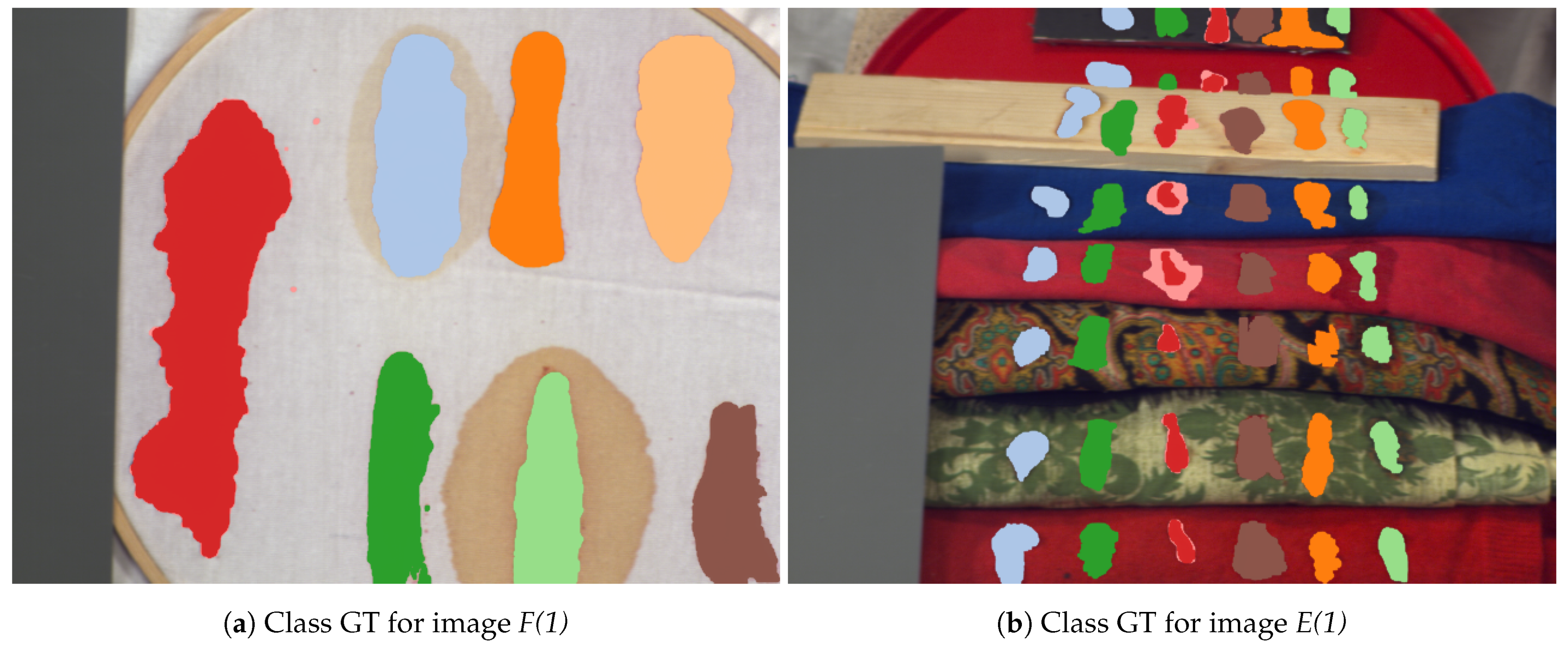
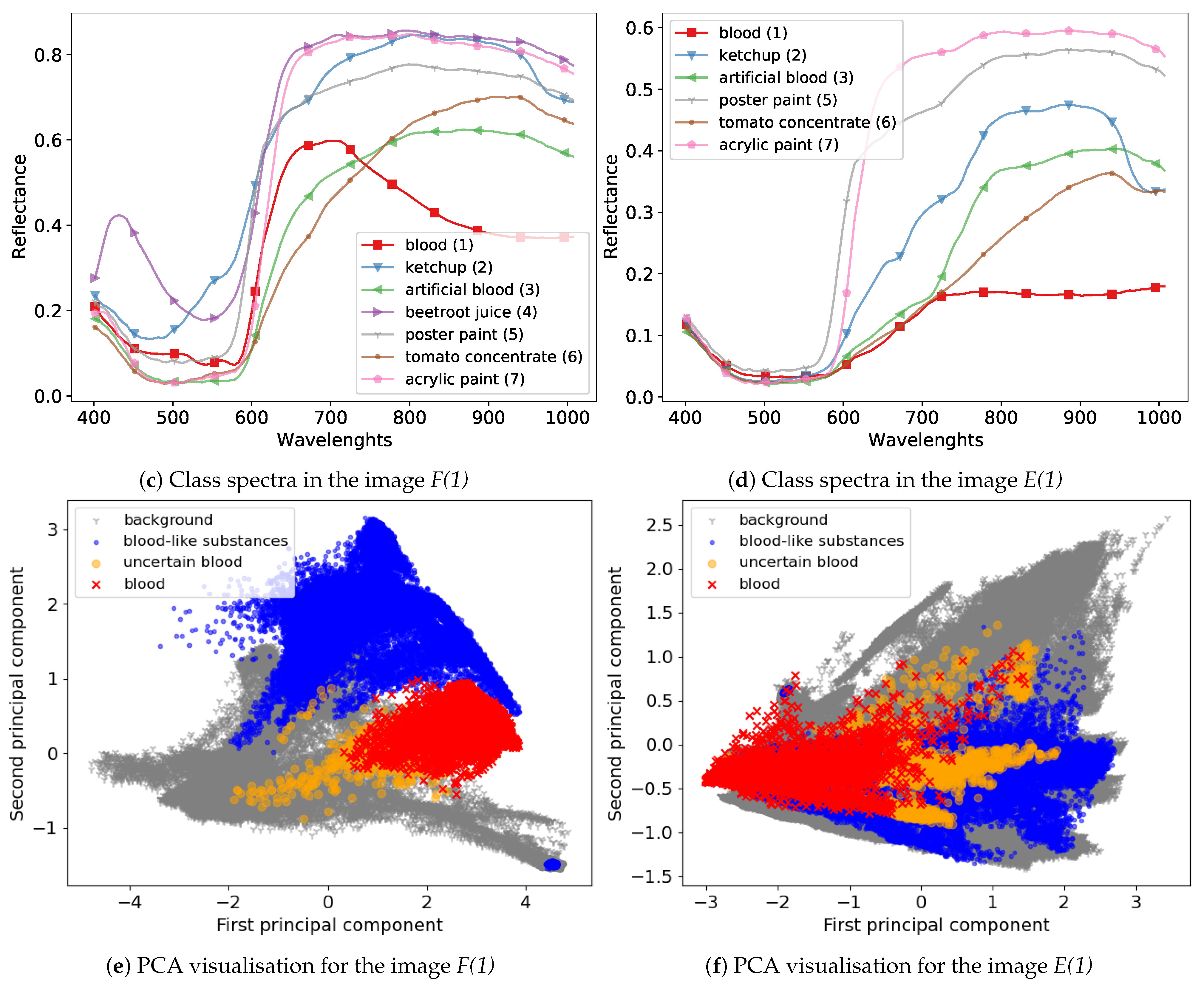
13]. To test both the HTC and HIC scenarios, in our experiments, we use a dataset described in [
14] that consists of multiple hyperspectral images with blood and blood-like substances. The dataset is inspired by problems related to forensic analysis; e.g., the detection of blood. However, we focus on the problem of classification; i.e., distinguishing between classes corresponding to visually similar blood-like substances in the images. We use multiple images with the same classes but with significant spectral differences to compare the HTC and the HIC scenarios. We analyse the impact of GAs on the classification accuracy in comparison to the grid-search parameter selection using multiple state-of-the-art hyperspectral classifiers.
Our thesis is that hyperspectral classification with a GA-based model and band selection would allow more accurate classifiers to be obtained compared to the approach when parameters are selected with GS. To test this, we compare the accuracy of classifiers optimised with GA and GS in both the transductive and inductive hyperspectral classification scenarios. Our main contribution is the identification and experimental verification of the conditions under which GA outperforms GS in hyperspectral classification. We show that in order for this advantage to be significant, the classification problem must be sufficiently complex, such as in the HIC scenario, which is more difficult compared to the HTC. In addition, the data in the validation set used for model selection must be sufficiently similar to data in the test set, which is not always the case in the HIC. Since the use of GA can be time consuming compared to GS, our conclusions allow for a more informed choice of model selection method in various hyperspectral classification problems.
2. State of the Art
Machine learning algorithms are currently popular and widely used in medical imaging [
15]. Some of the main areas of ML application are image segmentation—e.g., for melanin [
16] or epidermis [
17]—and segmentation and classification—e.g., for the detection of pigment network in dermoscopic images [
18]. Due to the visibility of haemoglobin in the spectra, hyperspectral imaging (HSI) has become useful in areas related to medical diagnosis [
19]. In addition, the detection and estimation of blood age in hyperspectral images [
20] can be applied to forensic analysis [
14]. However, the complexity of hyperspectral data makes the development of dedicated ML methods, especially classification algorithms, particularly important. Genetic algorithms are promising for the construction of hyperspectral classifiers as they enable simultaneous model selection and the reduction of data dimensionality.
2.1. Hyperspectral Classification
In this paper, we focus on spectral classification [
1] which uses only spectral vectors. The leading approaches involve the use of Support Vector Machines (SVMs) [
21], Extreme Learning Machines and their Kernel-based variants [
22] or Multinomial Logistic Regression [
23]. In order to further improve classification accuracy, spectral–spatial approaches [
24] are employed. They make use of both pixel spectra and their spatial position in the image. In particular, a combination of spatial–spectral and semi-supervised approaches allows a high classification accuracy to be obtained, even for a small training set [
5]. Recently, deep learning methods [
25] are popular, although their limiting factor is the fact that they usually require relatively large training sets. However, some works, such as the approach presented in [
26], based on residual networks, seem to be able to significantly reduce this dependency.
2.2. Evolutionary Computation and Genetic Algorithms
The advantages of techniques based on computational intelligence [
27] methods lie in the properties inherited from their biological counterparts: the learning and generalization of knowledge (artificial neural networks [
28]), global optimization (evolutionary computation [
29]) and the use of imprecise terms (fuzzy systems [
30]). The inspiration to undertake research on evolutionary computation (EC) [
29] was the imitation of nature in its mechanism of natural selection, inheritance and functioning. Genetic algorithms (GAs) [
31] are a part of evolutionary computation techniques, which have been used with success in fields such as the vehicle routing problem [
32], feature selection [
33], optimization [
34], heart sound segmentation [
35] or traveling salesman problem [
36].
Genetic algorithms are one of the leading approaches to solve optimisation problems [
9]. Due to the fact that they are computationally complex, they are often solved with heuristic methods, which make it possible to find a near-optimal solution faster. GA works by creating a population consisting of a selected number of individuals, each of them representing one solution to the problem. Then, from among all the individuals, those with the best results are selected and then subjected to genetic operators, which then create a new population. In particular, this technique can be applied for model selection to find parameters of a machine learning model and simultaneously perform feature selection, such as in works on heart arrhythmia detection [
37,
38], early diagnosis of hepatocellular cancer [
39] or the prediction of credit scoring [
40].
2.3. Hyperspectral Classification and Band Selection with GAs
GAs have been used many times for the classification and selection of characteristic wavelengths in hyperspectral data. For example, in [
10], the authors use GA to find small subsets of the most distinctive bands. In [
12], GAs are applied for band selection in preprocessed hyperspectral images in order to classify them. In [
41], GA optimization is used to divide hyperspectral bands into three classes related to their discriminative power in the classification task. Authors verify their results using three standard hyperspectral datasets; i.e., the “University of Pavia”, “Indian Pines” and “Hekla”. The use of GAs for the simultaneous optimization of SVM parameters and band selection in HSI classification is presented in [
13]. A similar scheme for multispectral data is used in [
11], in which the authors emphasize the advantage of genetic algorithms over parameter optimization using a grid search. A very interesting use of a GA is presented in [
42]: the authors apply a GA to a large number of hyperspectral cubes (111 images) in order to determine a subset of wavelengths characteristic for the identification of charcoal rot disease in soybean stems.
4. Experiments
The main idea behind our experiments was to perform model and feature selection with GA and compare these results with a diverse set of classifiers trained classically; i.e., with a grid-search. Referring to classification scenarios introduced in
Section 1, we considered three experimental scenarios:
Hyperspectral transductive classification (HTC)—training and test examples were randomly, uniformly selected from a single hyperspectral image.
Hyperspectral inductive classification (HIC)—training and test examples were selected from different images. Typically, training examples came from “Frame” images and testing examples came from the “Comparison” images.
Hyperspectral inductive classification with a validation Set (HICVS)—this scenario was similar to the HIC scenario: training examples came from “Frame” images and testing examples came from the “Comparison” images. However, model selection was performed using a separate validation set that was randomly, uniformly sampled from the “Comparison” scene. This scenario was designed to test the capabilities of GA optimisation under different conditions to those in the HIC scenario, which is discussed in detail in
Section 6.
4.1. The Scheme of Experiments
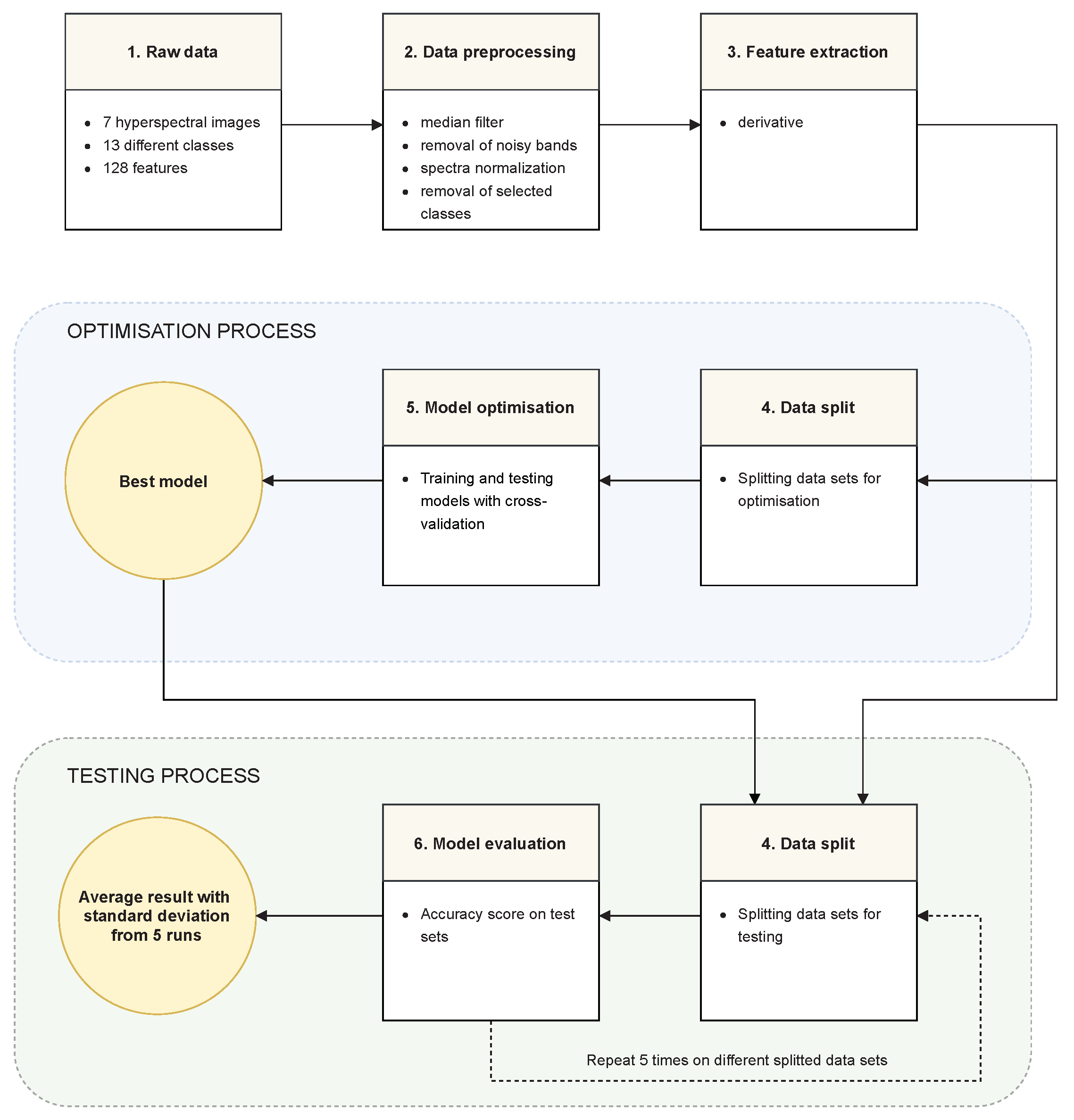
The experiments can be divided into six stages:
Raw data—The data set consisted of seven hyperspectral images from the data set described in
Section 3.1. Every image had 128 hyperspectral bands. The images represented two scenes—the “Frame” scene and the “Comparison” scene. Four of the seven images showed the “Frame” scene, captured in days
, where the value
represents the afternoon of the first day. The three “Comparison” images were captured on days
.
Data preprocessing—Data were transformed in accordance with the methodology described in
Section 3.2: in order to reduce the effect of noise and uneven lighting, spectra were smoothed with the median window, normalised and noisy bands were removed. Background (unannotated pixels) and pixels from the class “beetroot juice” (class 4) that was not present in all images were removed. Finally, the problem was posed as a six-class classification with classes
.
Feature extraction—A derivative transformation was used, as described in
Section 3.3.
Model optimization—Model and feature selection were performed as described in detail in
Section 3.5. The reference method used for comparison was a grid search. In both cases, the accuracy was chosen as the evaluation criterion. The settings and details of the cross-validation varied depending on the scenario of the experiment; detailed descriptions are provided in descriptions of the individual scenarios.
Model evaluation—The final final results were expressed in terms of classification accuracy. After finding the best model in stage 5, this model was trained on the entire training set and tested on the test sets. The test sets were created from both scenes: “Frame” and “Comparison”. The training and testing process was repeated five times and the average accuracy with the standard deviation was calculated.
An overview schema of our experiments based on the above steps is presented in
Figure 4. Transitions between successive stages are also described with a short summary of consecutive experiments phases.
4.2. Hyperspectral Transductive Classification (HTC)
In the HTC scenario training, pixels were randomly, uniformly sampled from the same images as test pixels. This scenario bore resemblance to a common hyperspectral classification setting, when classifiers are tested, e.g., using the “Indian Pines” data set [
1]. The aim of this experiment was to test the capability of classifiers to model classes and distinguish between them.
The training set was a combination of examples from all images; i.e., “Frame” and “Comparison” scenes from all days. The training set consisted of an equal number of examples from each class and each day. We used the size of the least numerous class among all the images (989); therefore, the training set consisted of 41,538 hyperspectral pixels (989 pixels * six classes * seven images).
After selecting the best parameters and features using cross-validation on the training set, classifiers were trained on the whole training set and tested on the remaining examples.
4.3. Hyperspectral Inductive Classification (HIC)
In the HIC scenario, classifiers were trained on “Frame” images and tested on “Comparison” images. This scenario simulated a potential forensic application, where the model was prepared using laboratory samples and applied in the field in an unknown environment.
The training set size was 6000 examples (250 examples from each class, from four available images). The test set consisted of a total of 82,097 examples from “Comparison” scenes.
Each model was optimized in the process of a 10-fold cross-validation as visualised in
Figure 5. Each time, one fold was used for training and the remaining ones for testing. Additionally, only a subset of 10 randomly selected examples from each class in the training set were used for training in a single cross-validation iteration. After the optimization stage, the best model was trained on examples in the training set and tested on the test set.
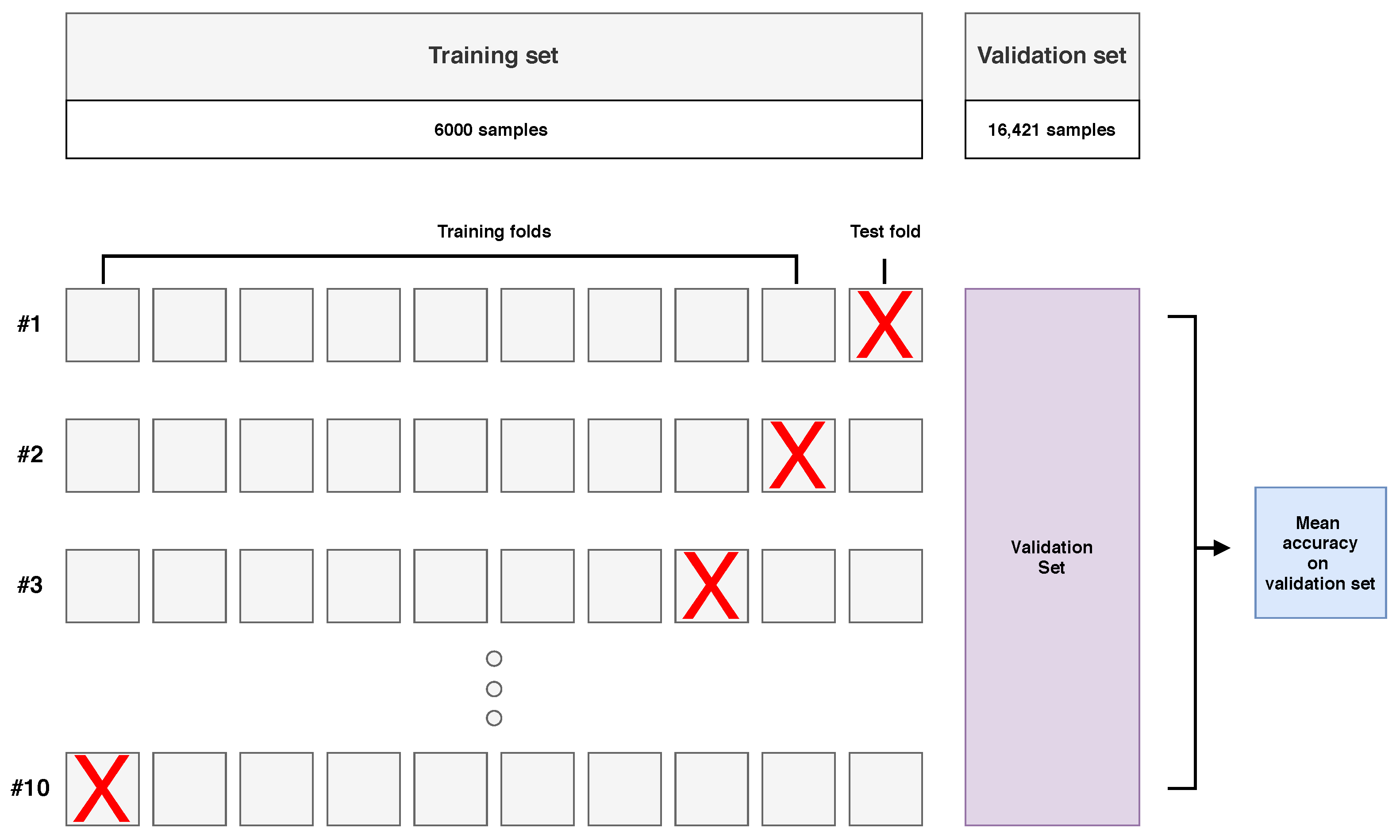
4.4. Hyperspectral Inductive Classification with a Validation Set (HICVS)
In the HICVS scenario, classifiers were trained on “Frame” images and tested on “Comparison” images, but in the model optimisation stage, a separate validation set was used, consisting of a subset of randomly, uniformly sampled examples from the “Comparison” images. The aim of this experiment was to determine and discuss the impact of applying GA in the model optimisation stage. The purpose was to test a scenario in which GA could perform the selection of features while maintaining model overfitting control. A discussion of this scenario is presented in the
Section 6.
In the experiment, all examples from tests scenes from all days were divided into a test and a validation set in a ratio of 80% to 20%. Similarly to the HIC scenario, pixels from test scenes were not used as training examples. However, during the model optimization stage, models were tested on the validation set. The test set consisted of 65,676 examples and the validation set consisted of 16,421 examples.
The training set contained 6000 examples (250 examples from each class, from four available images). Models were trained using 10-fold cross-validation, as presented in
Figure 6. Nine folds formed a training subset, and the model was tested on a validation set. The remaining fold was not involved in the validation process.
After the optimisation process, the best model was tested on a test set that did not contain examples from the validation set.
7. Conclusions and Future Works
We compared a GA-based model selection with the classic approach based on a grid search in three different hyperspectral classification scenarios. In the hyperspectral transductive classification (HTC) scenario, the training and test data were taken from a single image, so they were similar. For this scenario, if a sufficiently large training set was available, both methods of model selection achieved comparable, very high accuracy. In the hyperspectral inductive classification (HIC) scenario, the training and test data came from different images, which negatively affected the accuracy of all tested classifiers. In this scenario, GAs only gained an advantage over GS for some images; e.g., day 1 image, where the characteristic blood features associated with haemoglobin spectral response were most visible. The third scenario, i.e., the hyperspectral inductive classification with a validation set (HICVS), was created on the basis of the HIC scenario. In the HICVS scenario, the model selection algorithm had access to examples similar to those in the test set, which allowed the GA-based optimisation to outperform GS for all images.
Our results show that for noisy data, as in HIC, the advantage of GA over GS in terms of accuracy is not significant and that in order to achieve this advantage, GA must have examples representative of the test set at the model selection stage; e.g., in the HICVS scenario. On the other hand, for a typical HTC scenario, existing approaches such as [
5] or [
25] allow very high accuracy to be obtained without an extensive search of the parameter space. This suggests that GA is a promising solution to challenging problems of hyperspectral classification, but its effective use imposes certain requirements on the available training data. This problem shares similarities with the problem of domain adaptation, described, e.g., in [
55]. However, in all tested scenarios, the GA was able to generate models that were similar to or more accurate than GS while reducing the number of spectral bands by almost half.
We plan to apply the GA-based approach to different models, in particular recurrent neural networks, deep neural networks and ensemble learning. We would also like to test different feature extraction methods dedicated to the GA-based classification of hyperspectral images, especially in the HIC scenarios.


 ,
, 


