3.1. Optimization
The main purpose is to obtain a good sinusoidal magnetic field, which is to make the actual magnetic flux density consistent with the first harmonic of the magnetic flux density. As a result, the actual magnetic field has good sinusoidal characteristics, and the expression can be simplified as that of the first harmonic.
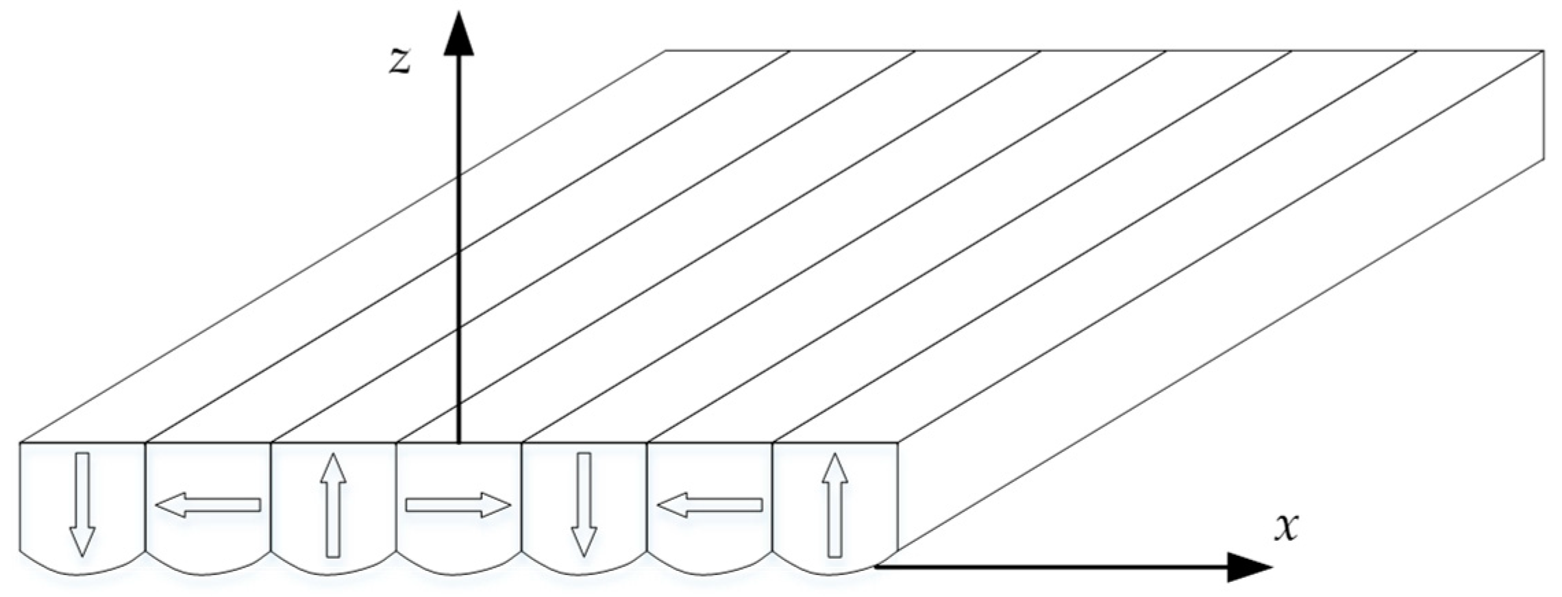
In the real-time control of electrical machines, the first harmonic of the magnetic flux density is usually used to calculate the force. The new magnet array is designed based on the conventional magnet array, and the shape of the surface is optimized. Therefore, the first harmonic of magnetic flux density of the conventional magnet array is chosen in the optimization.
The optimization is realized by reducing the higher harmonics. The shape of the curved surface is obtained by optimizing the height of small pieces. Generally, the main performance of the motors is reflected by the horizontal thrust. It is produced by the z component of the magnetic flux density. So the minimization of the higher harmonics of the z component is chosen to be the objective.
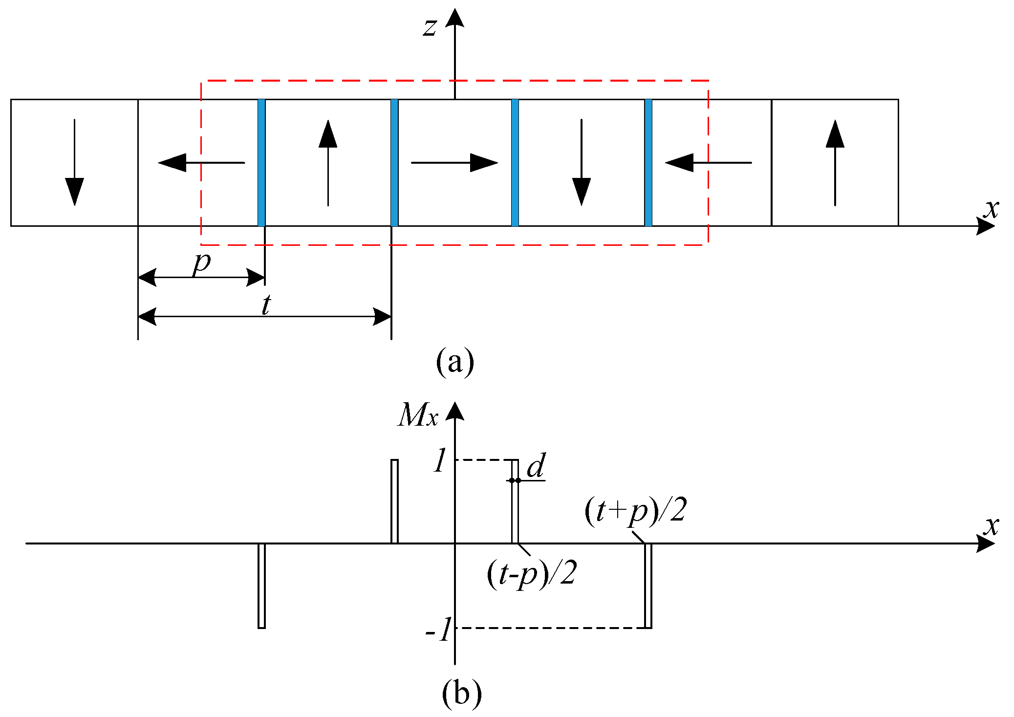
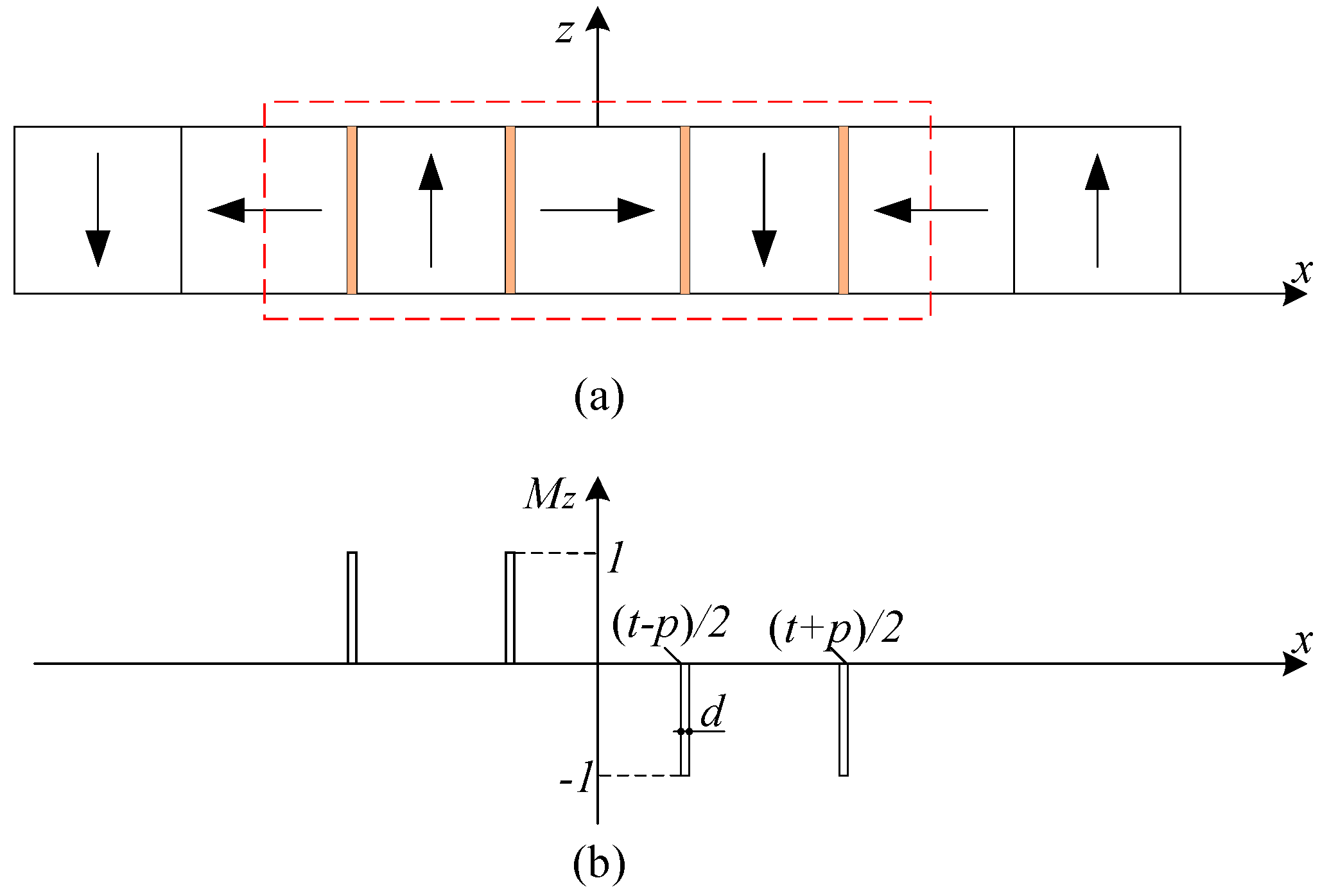
For the conventional magnet array, the first harmonic of the magnetic flux density can be obtained when
n takes 1 and expressed as
where
Bx1 and
Bz1 are the first harmonic of
x and
z component of magnetic flux density, respectively,
K1 is the coefficient,
mh is the height of the permanent magnet,
mt and
mb are the position of the top and bottom surfaces of the rectangular permanent magnet, respectively,
In order to determine the harmonic numbers for optimizing, we take the Br, t, p, and mh parameters of the permanent magnet as 1.2 T, 20 mm, 10 mm, and 10 mm for analysis, respectively. The maximum of the magnetic flux density at 2 mm below the x-axis is about 1.677 × 10⁻⁵ T when k = 25, which is much less than the geomagnetic field (about 6 × 10⁻⁵ T). The harmonic components can be ignored in optimization if the harmonic numbers, k, are more than 25.
Therefore, the approximate expression of the magnetic flux density can be represented by a certain number of harmonics. The
z component is given by
where
m = 25.
The higher harmonic components of the new magnet array can be evaluated by
According to the periodicity of the magnetic field, the region of half period is chosen. The region is placed 2 mm below the
x-axis and divided into 41 points. The objective function is given according to Equations (10) and (14)
where
xl = 0.025(
m − 1)
t and
zl = −0.002 are the coordinate values.
From the objective function, Equation (15), the reduction of higher harmonics is a constrained nonlinear multivariable optimization problem. The sequential quadratic programming (SQP) algorithm has the advantages of good convergence, high computational efficiency, and strong boundary searchability, which is chosen to realize the optimization. In order to avoid the singular points and obtain better optimization results, the number of pieces of half of one permanent magnet is set to five after analysis. For the whole permanent magnet, the total number of small pieces is 10. It is enough to exhibit well the shape of the curved surface of the permanent magnet.
The optimization parameters and variables are shown in
Table 1 and
Table 2, respectively. Considering the assembly of the permanent magnets, the positions of the top surface of each piece (
ht(1),
ht(2), …,
ht(5)) remain the same, and the optimization variables are the positions of the bottom surface of each piece of half of one permanent magnet (
hp(1),
hp(2), …,
hp(5)). The ‘constraints’ in
Table 2 define the range of optimization variables. Since the constraints of the five optimization variables are the same, they are represented by
hp(1)~
hp(5). Considering the optimization parameters, the upper bound of optimization variables does not exceed the position of the top surface of the small pieces, i.e., 10 mm. The lower bound of optimization variables does not exceed the position of the objective region, i.e., −2 mm.
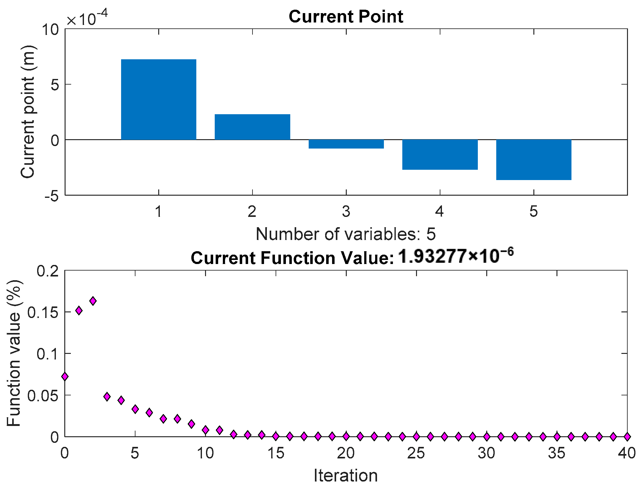
The results can be seen in
Figure 4, the minimization of the objective function is obtained. In
Figure 4, the ‘current point’ denotes the value of the optimization variables and is the best point the solver found in its run. The ‘current function value’ is the value of the objective function at the current point.
The small pieces of one permanent magnet based on the optimization variables are shown in
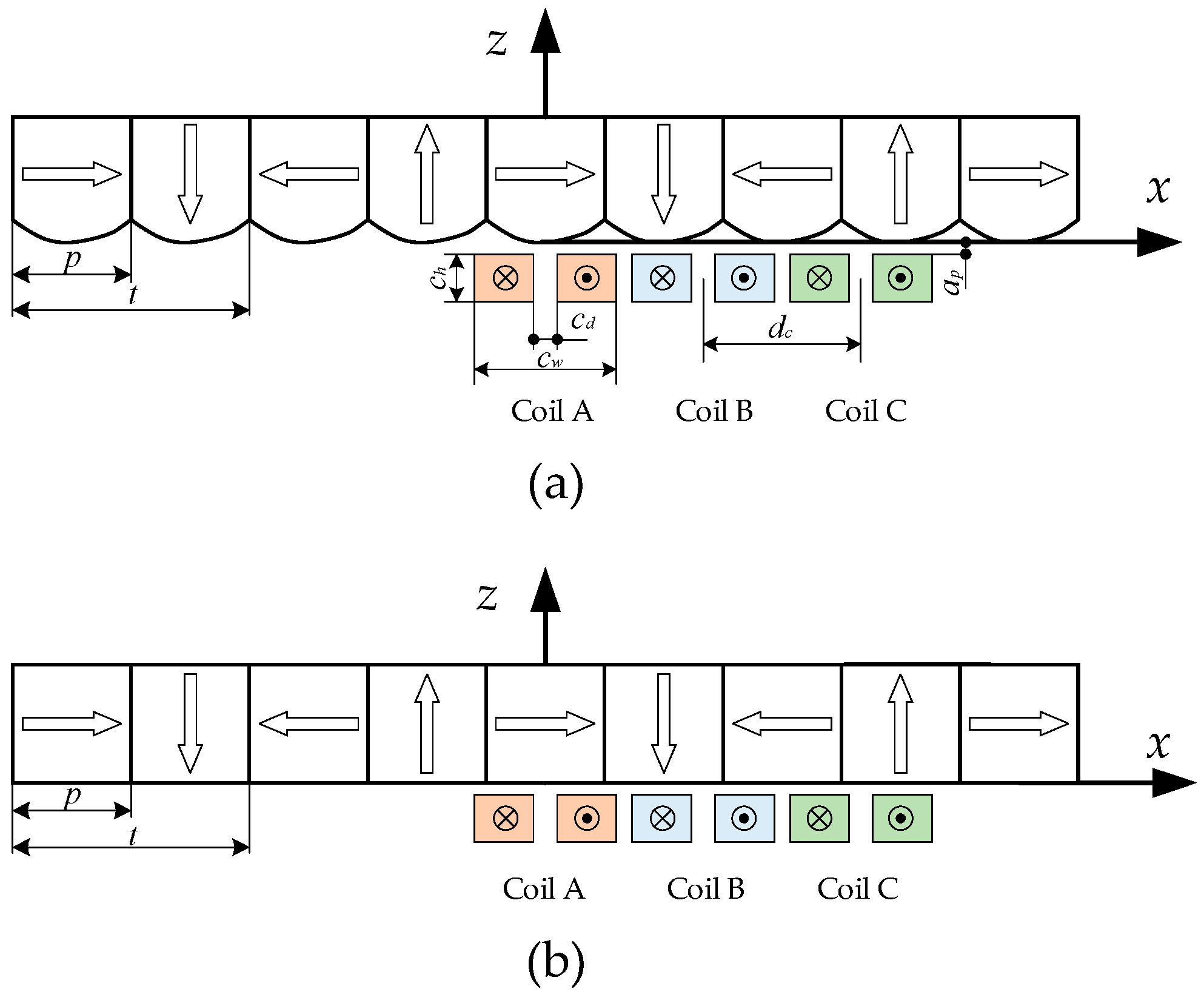
Figure 5. In the new magnet array, the optimized curved surfaces of permanent magnets in the
x and
z magnetization directions are the same. The symmetry axis of the curved surface is in the middle and both sides have a symmetrical distribution.
hp(1)~
hp(5) are the optimization variables and also the positions of bottom surfaces of small pieces of half of one permanent magnet. So the small pieces of one permanent magnet can be obtained according to symmetry.
We take the permanent magnet whose
x coordinate of the center is at zero as an example. The shape of the optimized curved surface of the permanent magnet is shown in
Figure 6. The data used to construct the curved surface shape are obtained according to the optimization results. It can be seen that the shape is similar to a sine or power function. The least squares polynomial fitting is used to fit the data. By comparing the results of a polynomial of degrees 2, 3, and 4, the fitting of the polynomial of degree 4 is more accurate. The polynomial of degree 4 is chosen. For better expression and without affecting the accuracy, the first- and third-order terms with very small coefficients are removed, and the sum of squares due to error (SSE) is 1.376 × 10
−10 m
2. The computed data of the polynomial is also shown in
Figure 6 and the expression is as follows
where
a1 = 3.763 × 10
5,
a2 = 34.28, and
a3 = −3.699 × 10
−4 are the coefficients, and the value range of
x is [−
p/2,
p/2].
According to the optimization and polynomial fitting, the analytical model of the magnetic flux density is simple and expressed as Equation (10).
3.2. Verification with FEM
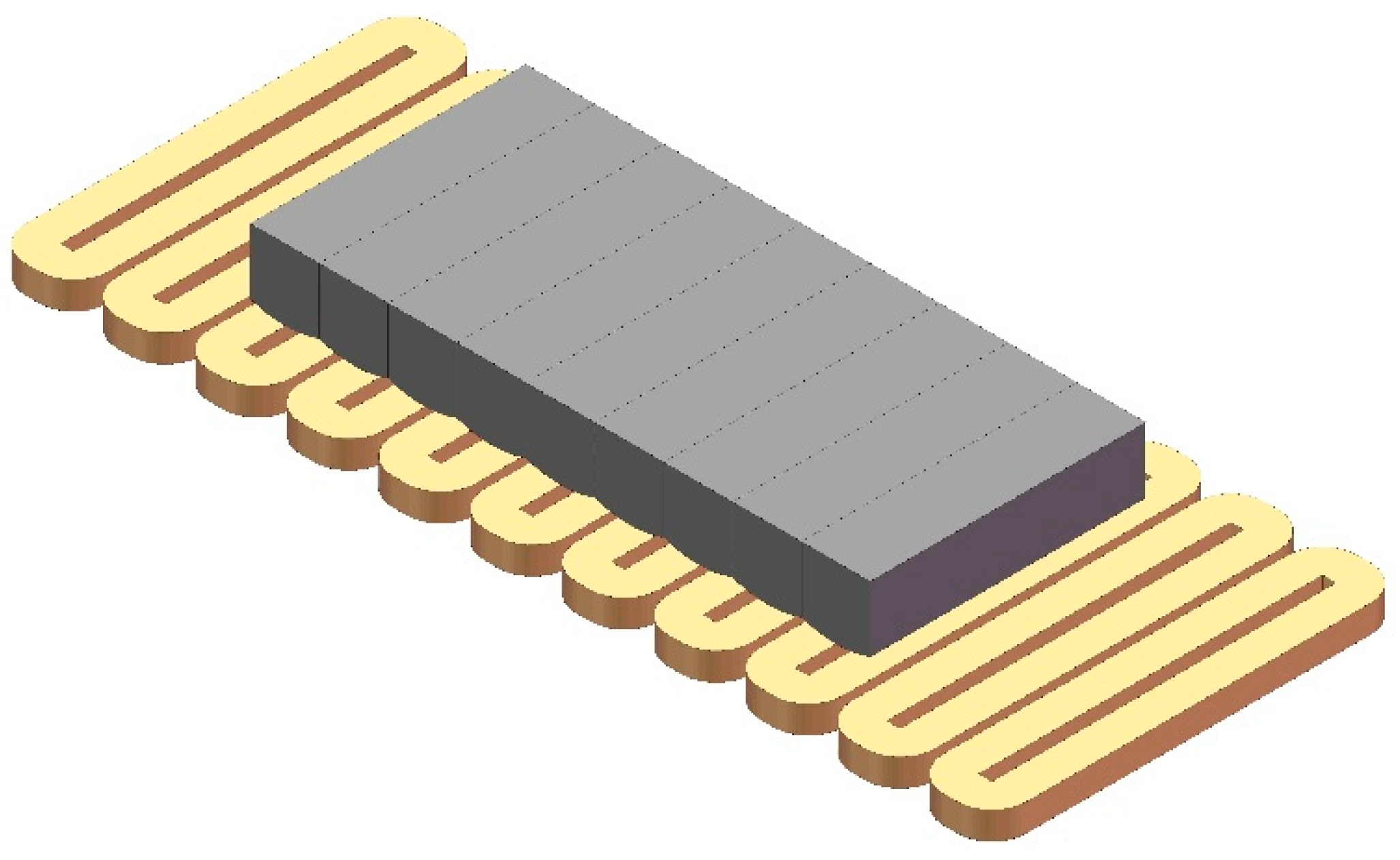
The new magnet array with a curved surface is obtained by applying the optimization results, and the axonometric drawing is shown in
Figure 7. In order to verify the optimization, the magnetic flux density with different
z coordinates are compared with the finite element model (FEM). The FEM is built and analyzed by the Ansoft Maxwell. With precision-driven adaptive subdivision technology and a powerful post-processor, Ansoft Maxwell is an excellent high-performance electromagnetic design software in the industry.
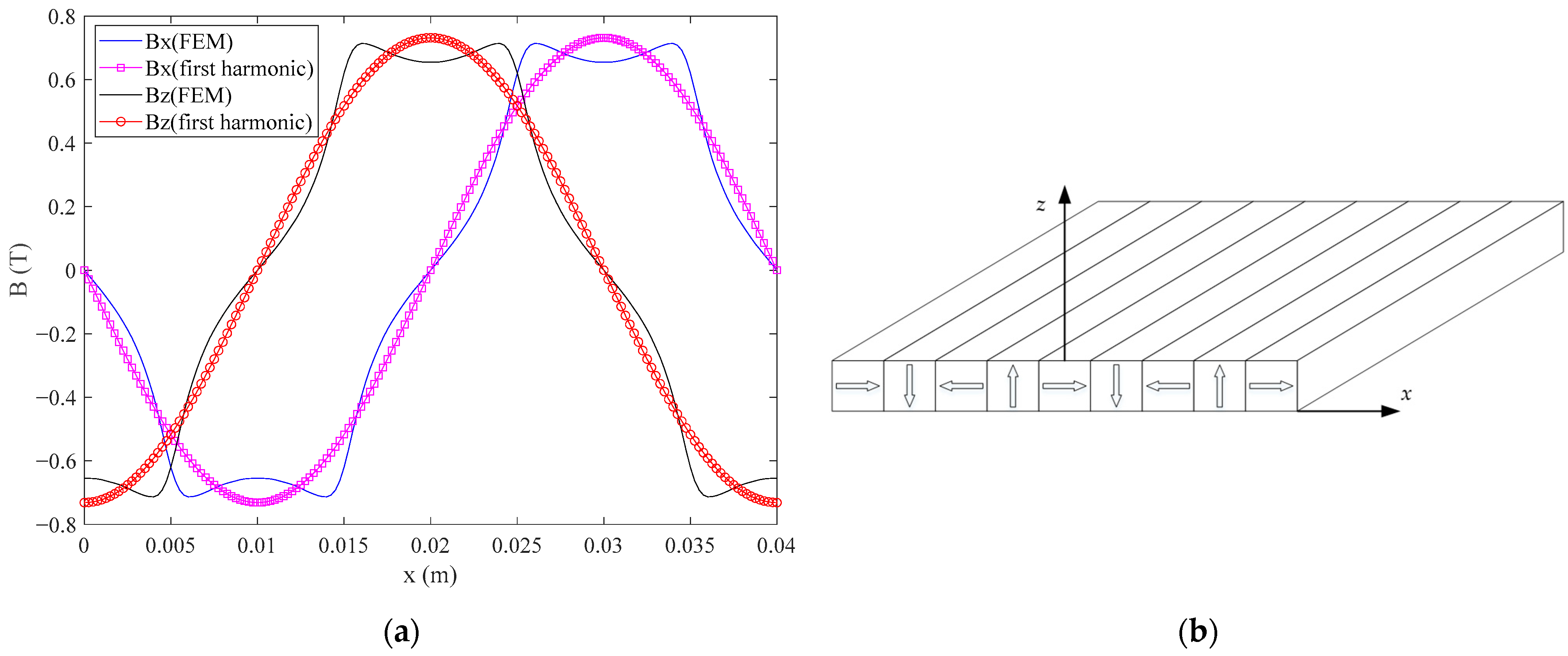
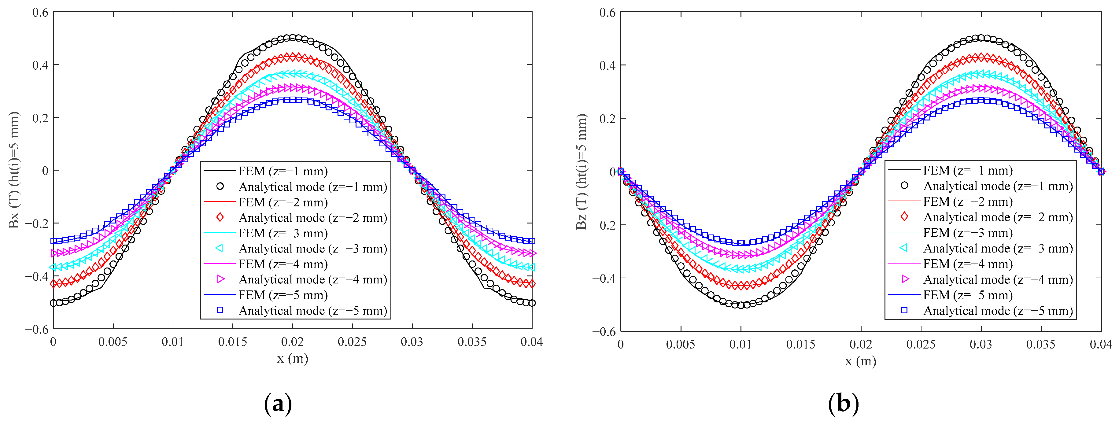
The magnetic flux density is obtained by the FEM and analytical model. The
x and
z components are shown in
Figure 8. It is found that the magnetic flux density has a good sinusoidal waveform. The analytical model results fit very well with the FEM results. The total harmonic distortion (THD) [
23] is introduced to evaluate the magnetic flux density. The root mean square (RMS) values of the error between the analytical model and FEM and THD of magnetic flux density are shown in
Table 3.
The RMS(ΔBx), RMS(ΔBz), THD(Bx) and THD(Bz) values for different z coordinates are very small. The maximum RMS(ΔBx) and RMS(ΔBz) values occurred when z is −1 mm, which are 2.19% and 2.14% of the peak value of Bx and Bz of FEM, respectively. The THD(Bx) and THD(Bz) values are the same according to Equation (7). The maximum THD(Bx) and THD(Bz) values occurred when z is −1 mm, which are both 2.69%. As a result, a new permanent magnet array with a good sinusoidal magnetic field and a simple analytical model of magnetic flux density is obtained.


