
Viscosity Measurement Sensor: A Prototype for a Novel Medical Diagnostic Method Based on Quartz Crystal Resonator

 , , ,
, , ,
Abstract
:
1. Introduction
2. Materials and Methods
2.1. Quartz Crystal Resonator
2.2. Measurement Setup
2.3. Samples
2.3.1. Artificial Synovial Fluid
2.3.2. Artificial Cerebrospinal Fluid
3. Results
3.1. Pure Fluids: Water, Alcohol, and Acetone
3.2. Test Dilutions: Glycerin, Sugar, and Salt Dilutions
3.3. aSF Results
3.4. aCSF Results
4. Discussion
5. Conclusions
Author Contributions
Funding
Institutional Review Board Statement
Informed Consent Statement
Data Availability Statement
Conflicts of Interest
References
- Brannan, S.R.; Jerrard, D.A. Synovial fluid analysis. J. Emerg. Med. 2006, 30, 331–339. [Google Scholar] [CrossRef] [PubMed]
- Stafford, C.T.; Niedermeier, W.; Holley, H.L.; Pigman, W. Studies on the concentration and intrinsic viscosity of hyaluronic acid in synovial fluids of patients with rheumatic diseases. Ann. Rheum. Dis. 1964, 23, 152–157. [Google Scholar] [CrossRef] [PubMed] [Green Version]
- Yetkin, F.; Kayabas, U.; Ersoy, Y.; Bayindir, Y.; Toplu, S.A.; Tek, I. Cerebrospinal fluid viscosity: A novel diagnostic measure for acute meningitis. South. Med. J. 2010, 103, 892–895. [Google Scholar] [CrossRef] [PubMed]
- Martinez-Castillo, A.; Núñez, C.; Cabiedes, J. Synovial fluid analysis. Reumatol. ClíNica 2010, 6, 316–321. [Google Scholar] [CrossRef]
- Sakka, L.; Coll, G.; Chazal, J. Anatomy and physiology of cerebrospinal fluid. Eur. Ann. Otorhinolaryngol. Head Neck Dis. 2011, 128, 309–316. [Google Scholar] [CrossRef] [Green Version]
- Damiano, J.; Bardin, T. Synovial fluid. EMC-Rhumatol.-Orthop. 2004, 1, 2–16. [Google Scholar] [CrossRef]
- Sangha, O. Epidemiology of rheumatic diseases. Rheumatology 2000, 39, 3–12. [Google Scholar] [CrossRef] [Green Version]
- Rojas, C. Estudio del Liquido Sinovial; Guías de Procedimientos en Reumatología: Bogotá, Colombia, 2011; pp. 41–47. [Google Scholar]
- West, S.G.; Kolfenbach, J. Rheumatology Secrets, 3rd ed.; Elsevier: Philadelphia, PA, USA, 2014. [Google Scholar]
- Wright, B.L.C.; Lai, J.T.F.; Sinclair, A.J. Cerebrospinal fluid and lumbar puncture: A practical review. J. Neurol. 2012, 259, 1530–1545. [Google Scholar] [CrossRef]
- Brouwer, M.C.; Tunkel, A.R.; van de Beek, D. Epidemiology, diagnosis, and antimicrobial treatment of acute bacterial meningitis. Clin. Microbiol. Rev. 2010, 23, 467–492. [Google Scholar] [CrossRef] [Green Version]
- Chadwick, D.R. Viral meningitis. Br. Med. Bull. 2005, 75–76, 1–14. [Google Scholar] [CrossRef]
- Dirri, F.; Palomba, E.; Longobardo, A.; Zampetti, E.; Saggin, B.; Scaccabarozzi, D. A review of quartz crystal microbalances for space applications. Sens. Actuators A Phys. 2019, 287, 48–75. [Google Scholar] [CrossRef]
- Wasilewski, T.; Szulczyński, B.; Wojciechowski, M.; Kamysz, W.; Gębicki, J. A Highly Selective Biosensor Based on Peptide Directly Derived from the HarmOBP7 Aldehyde Binding Site. Sensors 2019, 19, 4284. [Google Scholar] [CrossRef] [PubMed] [Green Version]
- Migoń, D.; Wasilewski, T.; Suchy, D. Application of QCM in Peptide and Protein-Based Drug Product Development. Molecules 2020, 25, 3950. [Google Scholar] [CrossRef] [PubMed]
- Huang, X.; Bai, Q.; Hu, J.; Hou, D. A practical model of quartz crystal microbalance in actual applications. Sensors 2017, 17, 1785. [Google Scholar] [CrossRef] [Green Version]
- Fort, A.; Panzardi, E.; Vignoli, V.; Tani, M.; Landi, E.; Mugnaini, M.; Vaccarella, P. An adaptive measurement system for the simultaneous evaluation of frequency shift and series resistance of QCM in liquid. Sensors 2021, 21, 678. [Google Scholar] [CrossRef]
- Kittle, J.; Levin, J.; Levin, N. Water Content of Polyelectrolyte Multilayer Films Measured by Quartz Crystal Microbalance and Deuterium Oxide Exchange. Sensors 2021, 21, 771. [Google Scholar] [CrossRef] [PubMed]
- Kömpf, D.; Held, J.; Müller, S.F.; Drechsel, H.R.; Tschan, S.C.; Northoff, H.; Gehring, F.K. Real-time measurement of Plasmodium falciparum-infected erythrocyte cytoadhesion with a quartz crystal microbalance. Malar. J. 2016, 15, 317. [Google Scholar] [CrossRef] [PubMed] [Green Version]
- Oberfrank, S.; Drechsel, H.; Sinn, S.; Northoff, H.; Gehring, F.K. Utilisation of quartz crystal microbalance sensors with dissipation (QCM-D) for a clauss fibrinogen assay in comparison with common coagulation reference methods. Sensors 2016, 16, 282. [Google Scholar] [CrossRef] [Green Version]
- Chen, Z.; Li, Q.; Chen, J.; Luo, R.; Maitz, M.F.; Huang, N. Immobilization of serum albumin and peptide aptamer for EPC on polydopamine coated titanium surface for enhanced in-situ self-endothelialization. Mater. Sci. Eng. C 2016, 60, 219–229. [Google Scholar] [CrossRef]
- Yang, Y.; Tu, Y.; Wang, X.; Pan, J.; Ding, Y. A label-free immunosensor for ultrasensitive detection of ketamine based on quartz crystal microbalance. Sensors 2015, 15, 8540–8549. [Google Scholar] [CrossRef] [PubMed] [Green Version]
- Kim, Y.K.; Lim, S.I.; Cho, Y.Y.; Choi, S.; Song, J.Y.; An, D.J. Detection of H3N2 canine influenza virus using a Quartz Crystal Microbalance. J. Virol. Methods 2014, 208, 16–20. [Google Scholar] [CrossRef] [PubMed]
- Lim, H.J.; Saha, T.; Tey, B.T.; Tan, W.S.; Ooi, C.W. Quartz crystal microbalance-based biosensors as rapid diagnostic devices for infectious diseases. Biosens. Bioelectron. 2020, 168, 112513. [Google Scholar] [CrossRef] [PubMed]
- Ash, D.C.; Joyce, M.J.; Barnes, C.; Booth, C.J.; Jefferies, A.C. Viscosity measurement of industrial oils using the droplet quartz crystal microbalance. Meas. Sci. Technol. 2003, 14, 1955. [Google Scholar] [CrossRef]
- Cao-Paz, A.M.; Rodríguez-Pardo, L.; Fariña, J.; Marcos-Acevedo, J. Resolution in QCM sensors for the viscosity and density of liquids: Application to lead acid batteries. Sensors 2012, 12, 10604–10620. [Google Scholar] [CrossRef] [PubMed]
- Tan, F.; Qiu, D.-Y.; Guo, L.-P.; Ye, P.; Zeng, H.; Jiang, J.; Zhang, Y.C. Separate density and viscosity measurements of unknown liquid using quartz crystal microbalance. Aip Adv. 2016, 6, 095313. [Google Scholar] [CrossRef] [Green Version]
- Ahumada, L.A.; González, M.X.; Sandoval, O.L.; Olmedo, J.J. Evaluation of Hyaluronic Acid Dilutions at Different Concentrations Using a Quartz Crystal Resonator (QCR) for the Potential Diagnosis of Arthritic Diseases. Sensors 2016, 16, 1959. [Google Scholar] [CrossRef] [Green Version]
- Sauerbrey, G. Verwendung von Schwingquarzen zur Wägung dünner Schichten und zur Mikrowägung. Z. für Phys. 1959, 155, 206–222. [Google Scholar] [CrossRef]
- Kanazawa, K.K.; Gordon, J.G., II. The oscillation frequency of a quartz resonator in contact with liquid. Anal. Chim. Acta 1985, 175, 99–105. [Google Scholar] [CrossRef]
- Johannsmann, D. Viscoelastic, mechanical, and dielectric measurements on complex samples with the quartz crystal microbalance. Phys. Chem. Chem. Phys. 2008, 10, 4516–4534. [Google Scholar] [CrossRef] [Green Version]
- Cassiède, M.; Daridon, J.L.; Paillol, J.H.; Pauly, J. Characterization of the behaviour of a quartz crystal resonator fully immersed in a Newtonian liquid by impedance analysis. Sens. Actuators A Phys. 2011, 167, 317–326. [Google Scholar] [CrossRef]
- Nakamoto, T.; Moriizumi, T. A Theory of a Quartz Crystal Microbalance Based upon a Mason Equivalent Circuit. Jpn. J. Appl. Phys. 1990, 29, 963–969. [Google Scholar] [CrossRef]
- Na Songkhla, S.; Nakamoto, T. Interpretation of Quartz Crystal Microbalance Behavior with Viscous Film Using a Mason Equivalent Circuit. Chemosensors 2021, 9, 9. [Google Scholar] [CrossRef]
- Songkhla, S.N.; Nakamoto, T. Signal Processing of Vector Network Analyzer Measurement for Quartz Crystal Microbalance With Viscous Damping. IEEE Sens. J. 2019, 19, 10386–10392. [Google Scholar] [CrossRef]
- Carvajal Ahumada, L.A.; Peña Pérez, N.; Herrera Sandoval, O.L.; del Pozo Guerrero, F.; Serrano Olmedo, J.J. A new way to find dielectric properties of liquid sample using the quartz crystal resonator (QCR). Sens. Actuators A Phys. 2016, 239, 153–160. [Google Scholar] [CrossRef]
- Open QCM. Available online: https://openqcm.com/about-openqcm-q-1 (accessed on 31 March 2021).
- Swan, A.; Amer, H.; Dieppe, P. The value of synovial fluid assays in the diagnosis of joint disease: A literature survey. Ann. Rheum. Dis. 2002, 61, 493–498. [Google Scholar] [CrossRef]
- Spector, R.; Snodgrass, S.R.; Johanson, C.E. A balanced view of the cerebrospinal fluid composition and functions: Focus on adult humans. Exp. Neurol. 2015, 273, 57–68. [Google Scholar] [CrossRef] [Green Version]
- Saini, M.; Sadhu, K.K. Two instantaneous fluorogenic steps for detection of nanomolar amyloid beta monomer and its interaction with stoichiometric copper(II) ion. Sens. Actuators B Chem. 2020, 303, 127086. [Google Scholar] [CrossRef]
- Rudell, J.B.; Rechs, A.J.; Jelman, T.J.; Ross-Inta, C.M.; Hao, S.; Gietzen, D.W. The Anterior Piriform Cortex Is Sufficient for Detecting Depletion of an Indispensable Amino Acid, Showing Independent Cortical Sensory Function. J. Neurosci. 2011, 31, 1583–1590. [Google Scholar] [CrossRef] [Green Version]
- Reguera, R.M. Interpretación del líquido cefalorraquídeo. An. Pediatr. Contin. 2014, 12, 30–33. [Google Scholar] [CrossRef]
- Codina, M.G.; de Cueto, M.; Vicente, D.; Echevarría, J.E.; Prats, G. Diagnóstico microbiológico de las infecciones del sistema nervioso central. Enfermedades Infecc. Microbiol. ClíNica 2011, 29, 127–134. [Google Scholar] [CrossRef]


| Fluid | H. A. Concentration (mg/mL) |
|---|---|
| Healthy aSF | 3.5 |
| aSF3 | 3.0 |
| aSF2 | 2.0 |
| OA aSF | 1.3 |
| aSF1 | 1.0 |
| RA aSF | 0.84 |
| Fluid | NaCl Concentration (mg/mL) | Concentration (mg/mL) | Albumin Concentration (mg/mL) |
|---|---|---|---|
| Healthy aCSF | 7.25 | 2.18 | 0.0 |
| VM aCSF | 7.25 | 2.18 | 0.5 |
| aCSF1 | 7.25 | 2.18 | 1.0 |
| aCSF2 | 7.25 | 2.18 | 2.0 |
| BM aCSF | 7.25 | 2.18 | 3.0 |
| Fluid | Density (Theory) (mg/mL) | Viscosity (Theory) (mPa · s) | ViSQCT | Open QCM® | ||||
|---|---|---|---|---|---|---|---|---|
(Hz) | Viscosity Obtained (mPa · s) | Difference Theory vs. ViSQCT (%) | (Hz) | Viscosity Obtained (mPa · s) | Difference Theory vs. Open QCM (%) | |||
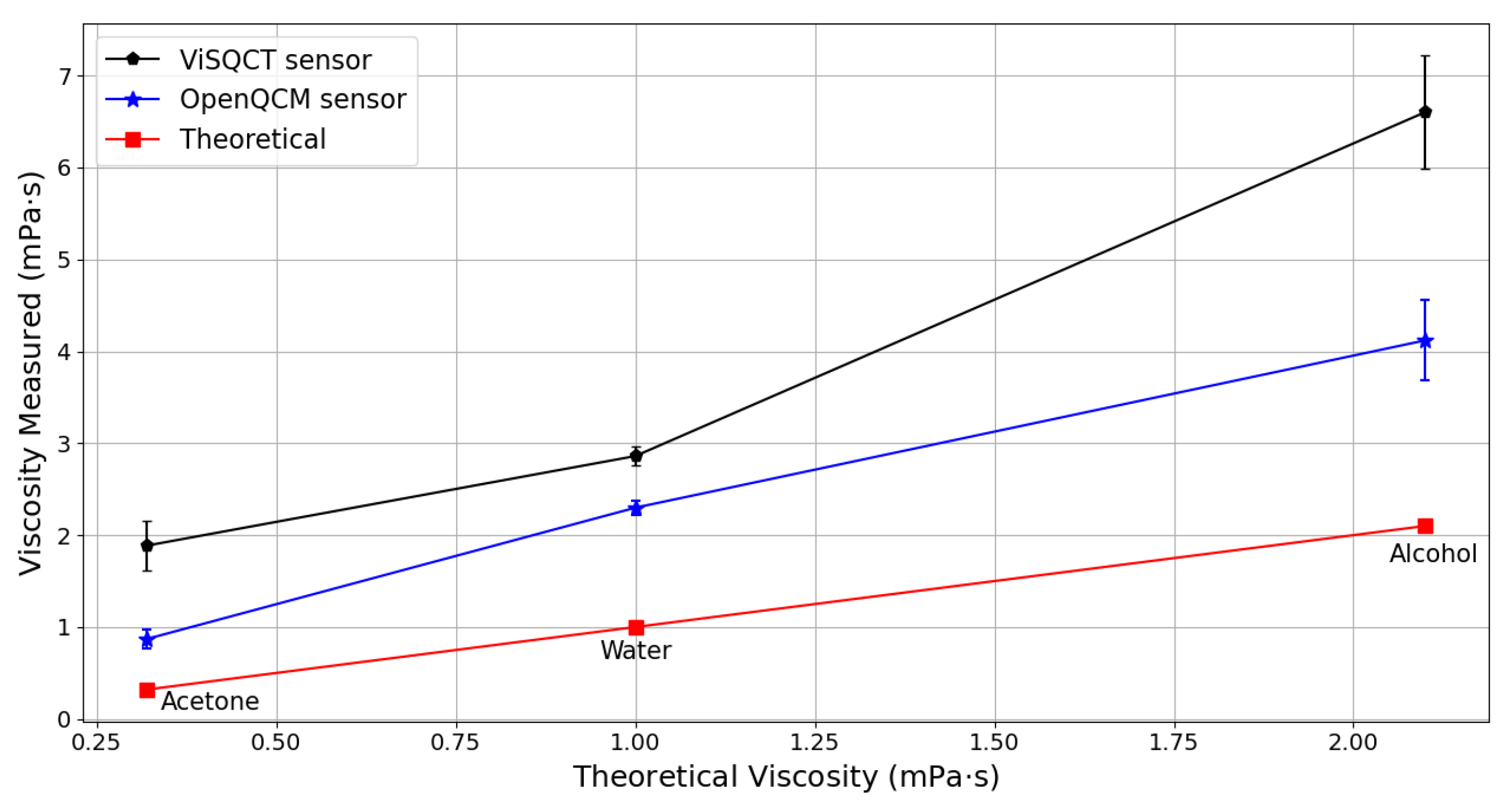
| Water | 1000 | 1.0 | 3416 ± 62 | 2.86 ± 0.10 | 186 | 3062 ± 54 | 2.298 ± 0.08 | 129 |
| Alcohol Isopropanol | 786 | 2.1 | 4601 ± 218 | 6.602 ± 0.62 | 214 | 3634 ± 196 | 4.119 ± 0.44 | 96 |
| Acetone | 791 | 0.32 | 2467 ± 179 | 1.886 ± 0.27 | 489 | 1676 ± 95 | 0.87 ± 0.10 | 171 |
| Fluid | Density (mg/mL) | Viscometer (mPa · s) | ViSQCT | Open QCM® | ||||
|---|---|---|---|---|---|---|---|---|
(Hz) | Viscosity Obtained (mPa · s) | Difference vs. Viscometer (%) | (Hz) | Viscosity Obtained (mPa · s) | Difference vs. Viscometer (%) | |||
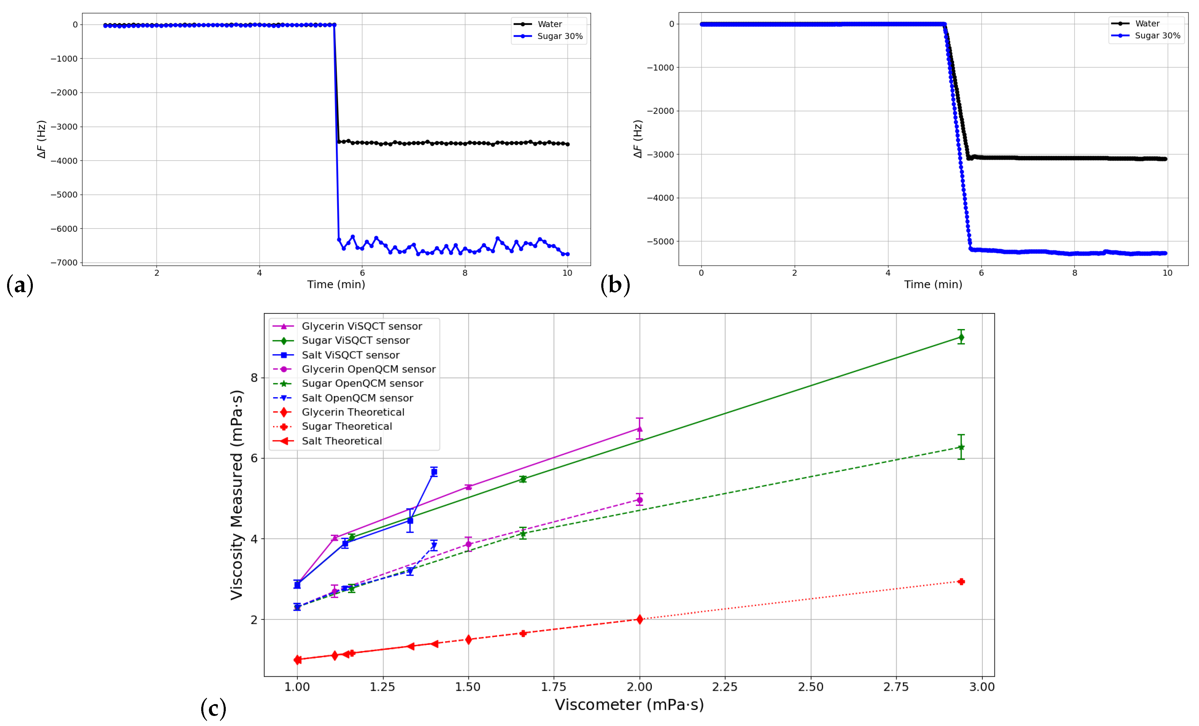
| Glycerin 10% | 1034 | 1.11 | 4115 ± 34 | 4.015 ± 0.06 | 261 | 3367 ± 95 | 2.687 ± 0.15 | 142 |
| Glycerin 20% | 1064 | 1.50 | 4789 ± 20 | 5.284 ± 0.04 | 252 | 4091 ± 96 | 3.856 ± 0.18 | 157 |
| Glycerin 30% | 1091 | 2.00 | 5475 ± 106 | 6.735 ± 0.26 | 236 | 4702 ± 67 | 4.968 ± 0.14 | 148 |
| Sugar 10% | 1045 | 1.16 | 4144 ± 46 | 4.028 ± 0.08 | 247 | 3432 ± 64 | 2.763 ± 0.10 | 138 |
| Sugar 20% | 1096 | 1.66 | 4949 ± 34 | 5.478 ± 0.07 | 230 | 4296 ± 74 | 4.128 ± 0.14 | 148 |
| Sugar 30% | 1139 | 2.94 | 6469 ± 65 | 9.007 ± 0.18 | 206 | 5398 ± 135 | 6.271 ± 0.30 | 113 |
| Salt 10% | 1088 | 1.14 | 4150 ± 64 | 3.880 ± 0.12 | 240 | 3502 ± 25 | 2.763 ± 0.04 | 142 |
| Salt 20% | 1145 | 1.33 | 4557 ± 149 | 4.446 ± 0.29 | 234 | 3855 ± 56 | 3.182 ± 0.09 | 139 |
| Salt 30% | 1194 | 1.40 | 5249 ± 52 | 5.657 ± 0.11 | 304 | 4317 ± 76 | 3.826 ± 0.13 | 173 |
| H. A. Concentration (mg/mL) | Density (mg/mL) | Viscosity (mPa · s) | ViSQCT | Open QCM® | ||||
|---|---|---|---|---|---|---|---|---|
| || (Hz) | Viscosity Obtained (mPa · s) | Difference vs. Viscometer (%) | || (Hz) | Viscosity Obtained (mPa · s) | Difference vs. Viscometer (%) | |||
| 0.84 (RA aSF) | 1007 | 94 | 3322 ± 31 | 2.686 ± 0.05 | 97 | 3103 ± 88 | 2.344 ± 0.13 | 97 |
| 1.0 | 1008 | 109 | 3417 ± 36 | 2.839 ± 0.06 | 97 | 3104 ± 99 | 2.343 ± 0.15 | 98 |
| 1.3 (OA aSF) | 1009 | 141 | 3439 ± 34 | 2.873 ± 0.06 | 98 | 3170 ± 75 | 2.441 ± 0.11 | 98 |
| 2.0 | 1013 | 342 | 3468 ± 48 | 2.91 ± 0.08 | 99 | 3146 ± 70 | 2.395 ± 0.10 | 99 |
| 3.0 | 1022 | 716 | 3525 ± 54 | 2.98 ± 0.10 | 99 | 3162 ± 78 | 2.398 ± 0.12 | 99 |
| 3.5 (Healthy aSF) | 1028 | 1133 | 3569 ± 69 | 3.037 ± 0.11 | 99 | 3216 ± 77 | 2.466 ± 0.12 | 99 |
| Fitting Curve Type | Function | Parameters | RMSE |
|---|---|---|---|
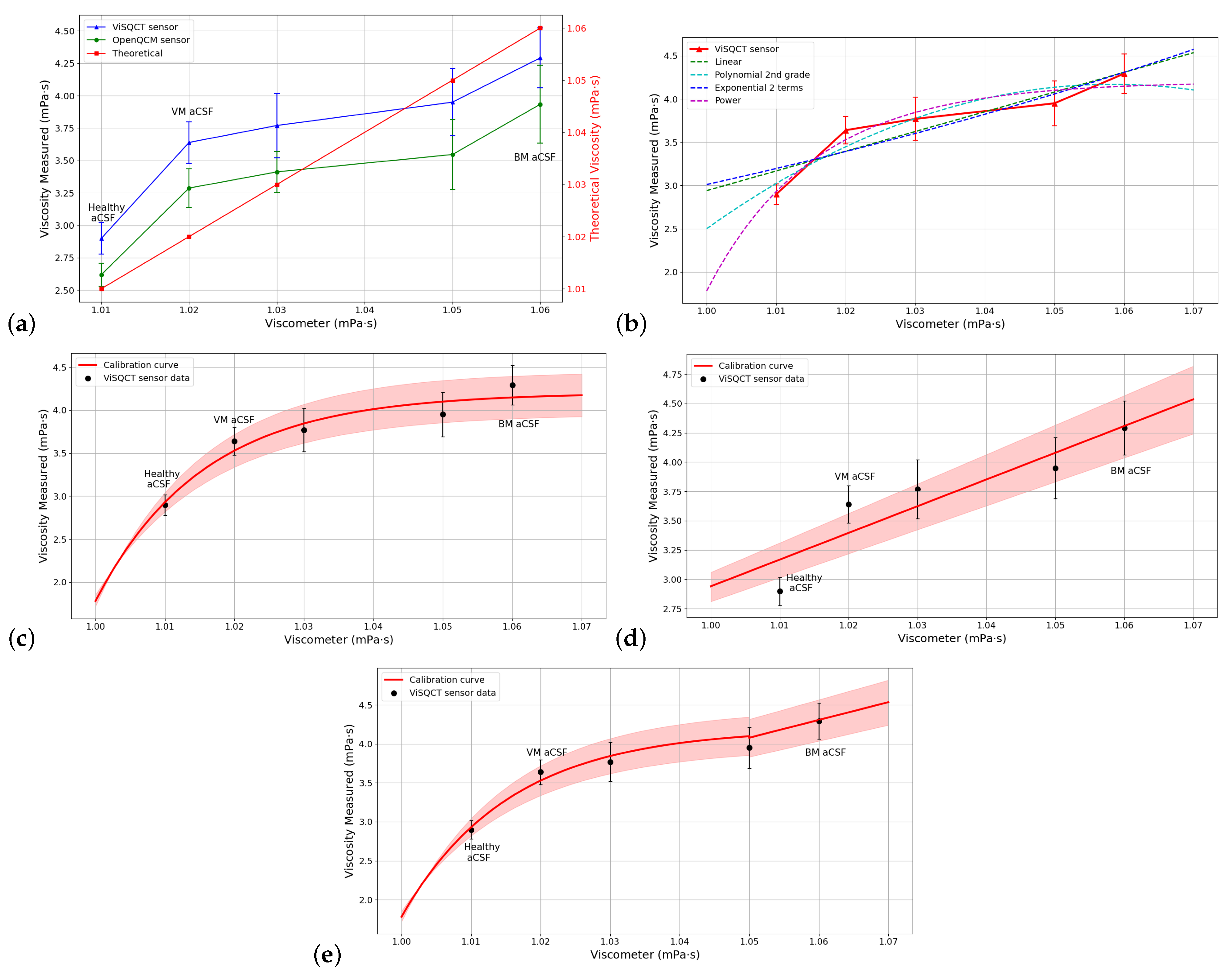
| Linear | f(x) = ax + b | a = b = 2.784 | 0.0728 |
| Polynomial 2nd grade | f(x) = + bx + c | a = b = c = 2.737 | 0.0747 |
| Exponential (2 terms) | a = 2.855 b = c = −7414 d = −0.1128 | 0.0073 | |
| Power | a = b = −2.438 c = 2.984 | 0.0563 |
| H. A. Concentration (mg/mL) | Viscosity Obtained (mPa · s) | Viscosity Calibrated (mPa · s) | Viscosity with Viscometer (mPa · s) | Error (%) |
|---|---|---|---|---|
| 0.84 (RA aSF) | 2.686 | 94.007 | 94 | 0.007 |
| 1.0 | 2.839 | 109.13 | 109 | 0.119 |
| 1.3 (OA aSF) | 2.873 | 130.70 | 141 | 7.305 |
| 2.0 | 2.91 | 341.50 | 342 | 0.146 |
| 3.0 | 2.98 | 767.00 | 716 | 7.123 |
| 3.5 (Healthy aSF) | 3.037 | 1106.00 | 1133 | 2.383 |
| H. A. Concentration (mg/mL) | Density (mg/mL) | Viscosity (mPa · s) | ViSQCT | Open QCM® | ||||
|---|---|---|---|---|---|---|---|---|
| || (Hz) | Viscosity Obtained (mPa · s) | Difference vs. Viscometer (%) | || (Hz) | Viscosity Obtained (mPa · s) | Difference vs. Viscometer (%) | |||
| 0.0 (aCSF) | 1008 | 1.01 | 3452 ± 75 | 2.898 ± 0.12 | 187 | 3281 ± 61 | 2.618 ± 0.09 | 159 |
| 0.5 (VM aCSF) | 1010 | 1.02 | 3872 ± 86 | 3.639 ± 0.16 | 256 | 3680 ± 88 | 3.287 ± 0.15 | 222 |
| 1.0 | 1012 | 1.03 | 3945 ± 134 | 3.77 ± 0.25 | 266 | 3753 ± 91 | 3.412 ± 0.16 | 231 |
| 2.0 | 1013 | 1.05 | 4040 ± 136 | 3.95 ± 0.26 | 276 | 3828 ± 145 | 3.546 ± 0.27 | 237 |
| 3.0 (BM aCSF) | 1017 | 1.06 | 4220 ± 118 | 4.292 ± 0.23 | 285 | 4040 ± 182 | 3.934 ± 0.30 | 271 |
| Fitting Curve Type | Function | Parameters | RMSE |
|---|---|---|---|
| Linear | f(x) = ax + b | a = 22.8 b = −19.86 | 0.2382 |
| Polynomial 2nd grade | a = −489.9 b = 1037 c = −544.6 | 0.2253 | |
| Exponential (2 terms) | a = 0.00768 b = 5.971 c = 0 d = −216.9 | 0.4358 | |
| Power | a = −2.422 b = −64.6 c = 4.203 | 0.1760 |
| Albumin (mg/mL) | Viscosity Obtained (mPa · s) | Viscosity Calibrated (mPa · s) | Viscosity with Viscometer (mPa · s) | Error (%) |
|---|---|---|---|---|
| 0.0 (aCSF) | 2.898 | 1.009 | 1.01 | 0.099 |
| 0.5 (VM aCSF) | 3.639 | 1.022 | 1.02 | 0.196 |
| 1.0 | 3.77 | 1.027 | 1.03 | 0.291 |
| 2.0 | 3.95 | 1.035 | 1.05 | 1.428 |
| 3.0 (BM aCSF) | 4.292 | 1.059 | 1.06 | 0.094 |
Publisher’s Note: MDPI stays neutral with regard to jurisdictional claims in published maps and institutional affiliations. |
© 2021 by the authors. Licensee MDPI, Basel, Switzerland. This article is an open access article distributed under the terms and conditions of the Creative Commons Attribution (CC BY) license (https://creativecommons.org/licenses/by/4.0/).
Share and Cite
Miranda-Martínez, A.; Rivera-González, M.X.; Zeinoun, M.; Carvajal-Ahumada, L.A.; Serrano-Olmedo, J.J. Viscosity Measurement Sensor: A Prototype for a Novel Medical Diagnostic Method Based on Quartz Crystal Resonator. Sensors 2021, 21, 2743. https://doi.org/10.3390/s21082743
Miranda-Martínez A, Rivera-González MX, Zeinoun M, Carvajal-Ahumada LA, Serrano-Olmedo JJ. Viscosity Measurement Sensor: A Prototype for a Novel Medical Diagnostic Method Based on Quartz Crystal Resonator. Sensors. 2021; 21(8):2743. https://doi.org/10.3390/s21082743
Chicago/Turabian StyleMiranda-Martínez, Andrés, Marco Xavier Rivera-González, Michael Zeinoun, Luis Armando Carvajal-Ahumada, and José Javier Serrano-Olmedo. 2021. "Viscosity Measurement Sensor: A Prototype for a Novel Medical Diagnostic Method Based on Quartz Crystal Resonator" Sensors 21, no. 8: 2743. https://doi.org/10.3390/s21082743
APA StyleMiranda-Martínez, A., Rivera-González, M. X., Zeinoun, M., Carvajal-Ahumada, L. A., & Serrano-Olmedo, J. J. (2021). Viscosity Measurement Sensor: A Prototype for a Novel Medical Diagnostic Method Based on Quartz Crystal Resonator. Sensors, 21(8), 2743. https://doi.org/10.3390/s21082743