
Sensor Data Fusion for a Mobile Robot Using Neural Networks


 ,
,  ,
,  and
and
Abstract
:
1. Introduction
2. Materials and Methods
2.1. Ultrasonic Sensor
Kalman Filter
2.2. Stereo Camera
2.3. LiDAR
2.4. Homogeneous Transformation Matrices
2.5. Data Fusion
2.6. Deep Feed forward Neural Networks
2.6.1. Gradient Stochastic Descent Optimizer
2.6.2. Neural Network Configuration
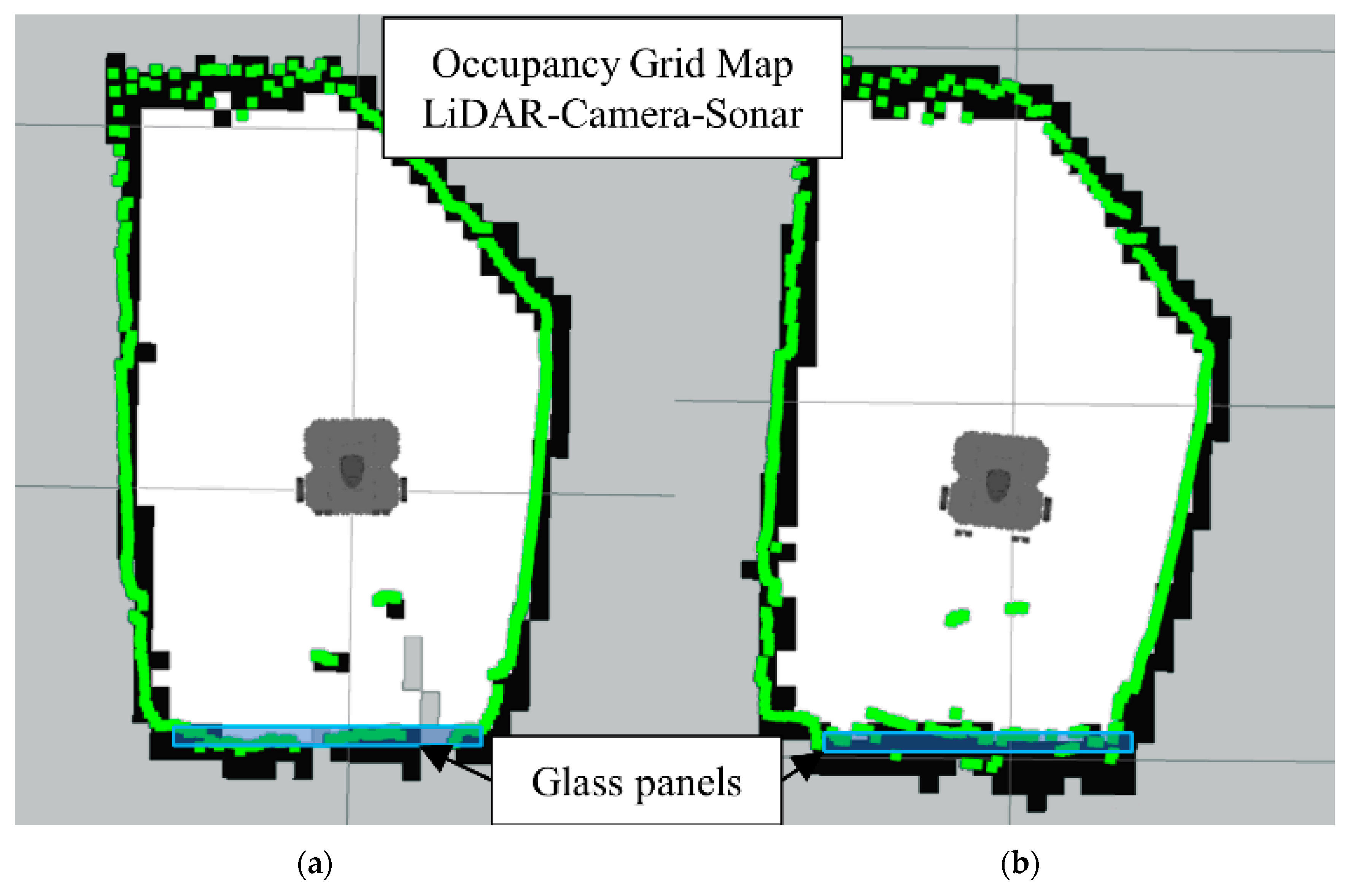
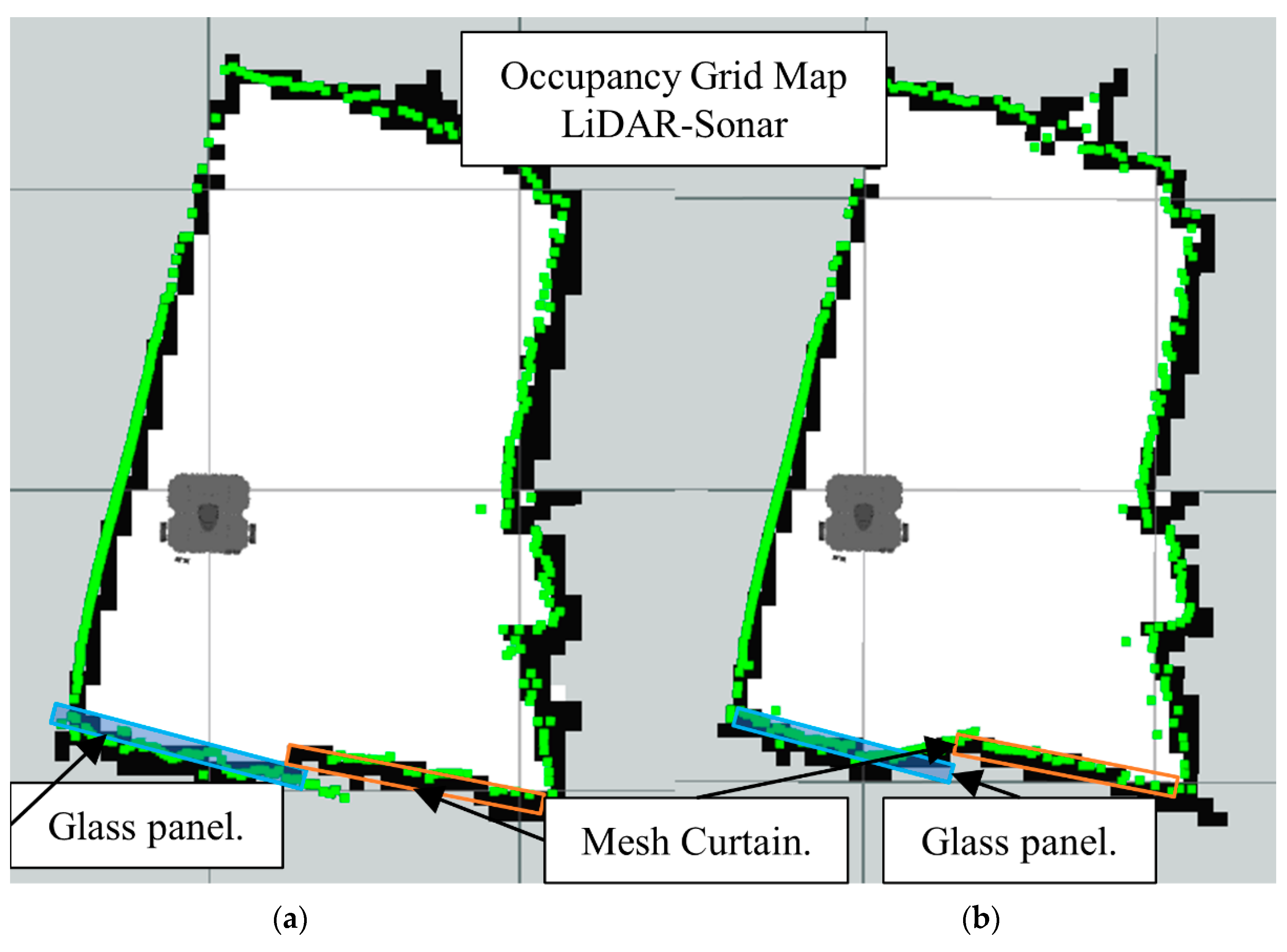
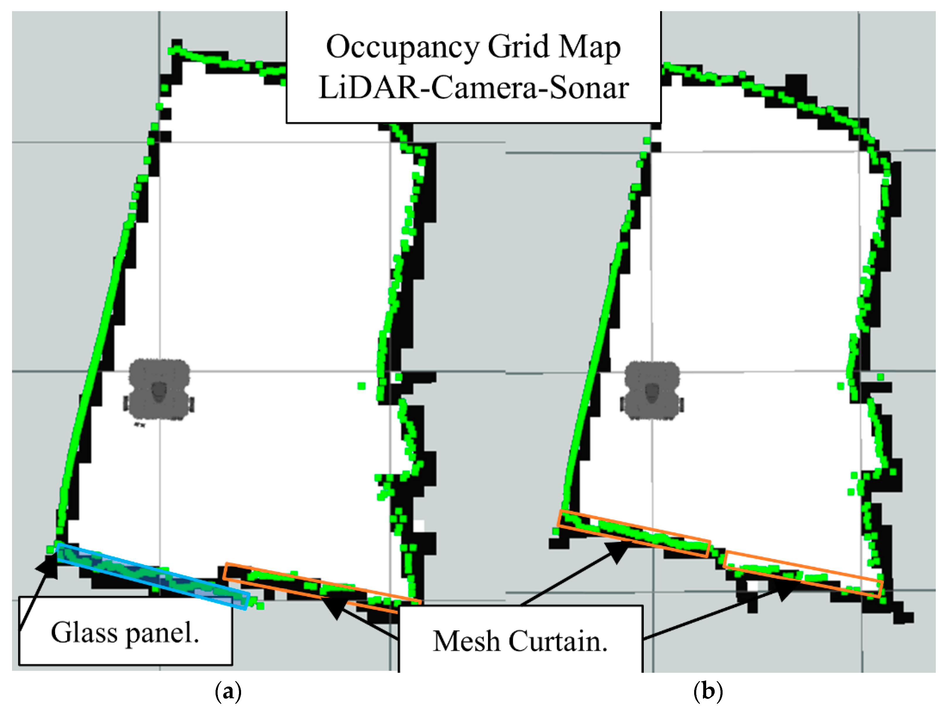
2.7. Occupancy Grid Map
3. Experimental Setup
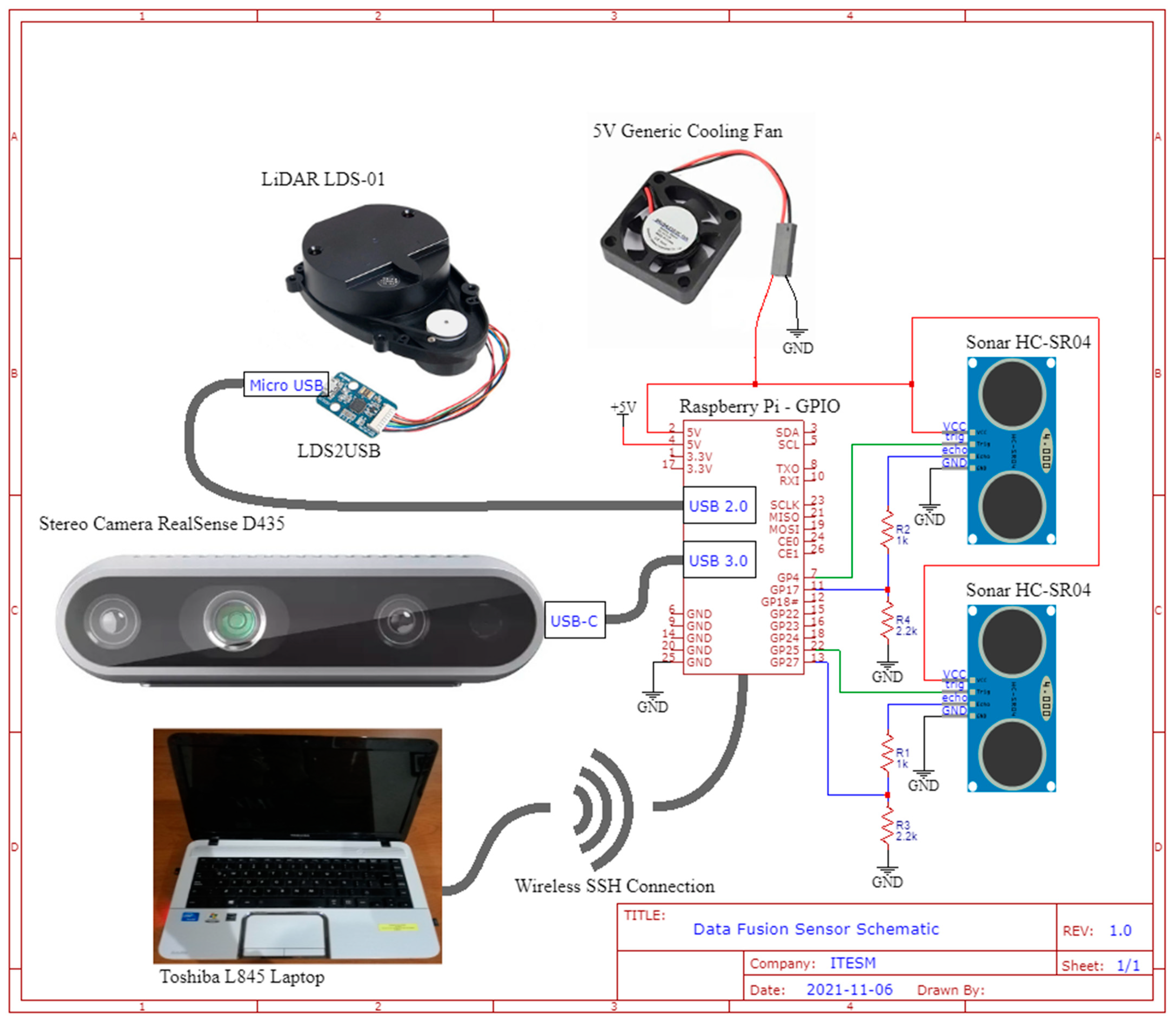
3.1. Hardware
3.2. Proving Ground
3.3. Software
3.3.1. Remote Server (Raspberry Pi 4)
3.3.2. Main Processing Unit (Toshiba Satellite L845 Laptop)
3.4. Training and Running the Network
4. Results
4.1. Scenario 1
4.2. Scenario 2
4.3. Scenario 3
5. Conclusions
Author Contributions
Funding
Institutional Review Board Statement
Informed Consent Statement
Acknowledgments
Conflicts of Interest
References
- Data Fusion Lexicon “The Data Fusion Subpanel of the Joint Directors of Laboratories, Technical Panel for C3 v}. 1991. Available online: https://apps.dtic.mil/sti/pdfs/ADA529661.pdf (accessed on 23 March 2020).
- Castanedo, F. A Review of Data Fusion Techniques. Sci. World J. 2013, 2013, 704504. [Google Scholar] [CrossRef] [PubMed]
- Xu, J.; Yang, G.; Sun, Y.; Picek, S. A Multi- Sensor Information Fusion Method Based on Factor Graph for Integrated Navigation System. IEEE Access 2021, 9, 12044–12054. [Google Scholar] [CrossRef]
- Kubelka, V.; Reinstein, M.; Svoboda, T. Improving multimodal data fusion for mobile robots by trajectory smoothing. Robot. Auton. Syst. 2016, 84, 88–96. [Google Scholar] [CrossRef]
- Wu, J.K.; Wong, Y.F. Bayesian approach for data fusion in sensor networks. In Proceedings of the 2006 9th International Conference on Information Fusion, Florence, Italy, 10–13 July 2006; Volume 1. Available online: https://www.proceedings.com/content/001/001016webtoc.pdf (accessed on 20 February 2020). [CrossRef]
- Buonocore, L.; Almeida, A.D.; Neto, C.L.N. A sensor data fusion algorithm for indoor slam using a low-cost mobile robot. Adapt. Mob. Robot. 2012, 2012, 762–769. [Google Scholar]
- Wei, P.; Cagle, L.; Reza, T.; Ball, J.; Gafford, J. LiDAR and Camera Detection Fusion in a Real-Time Industrial Multi- Sensor Collision Avoidance System. Electronics 2018, 7, 84. [Google Scholar] [CrossRef] [Green Version]
- Yi, Z.; Yuan, L. Application of fuzzy neural networks in data fusion for mobile robot wall-following. In Proceedings of the 2008 7th World Congress on Intelligent Control and Automation, Chongqing, China, 25–27 June 2008; pp. 6575–6579. [Google Scholar]
- Parasuraman, S. Sensor Fusion for Mobile Robot Navigation: Fuzzy Associative Memory. Procedia Eng. 2012, 41, 251–256. [Google Scholar] [CrossRef]
- Asvadi, A.; Garrote, L.; Premebida, C.; Peixoto, P.; Nunes, U.J. Multimodal vehicle detection: Fusing 3D-LIDAR and color camera data. Pattern Recognit. Lett. 2018, 115, 20–29. Available online: https://www.researchgate.net/publication/320089205_Multimodal_vehicle_detection_Fusing_3D-LIDAR_and_color_camera_data (accessed on 20 February 2020). [CrossRef]
- VPopov, L.; Ahmed, S.A.; Topalov, A.V.; Shakev, N.G. Development of Mobile Robot Target Recognition and Following Behaviour Using Deep Convolutional Neural Network and 2D Range Data. IFAC-PapersOnLine 2018, 51, 210–215. Available online: https://www.researchgate.net/publication/329148363_Development_of_Mobile_Robot_Target_Recognition_and_Following_Behaviour_Using_Deep_Convolutional_Neural_Network_and_2D_Range_Data (accessed on 20 February 2020). [CrossRef]
- Lv, M.; Xu, W.; Chen, T. A hybrid deep convolutional and recurrent neural network for complex activity recognition using multimodal sensors. Neurocomputing 2019, 362, 33–40. Available online: https://www.researchgate.net/publication/334538447_A_Hybrid_Deep_Convolutional_and_Recurrent_Neural_Network_for_Complex_Activity_Recognition_Using_Multimodal_Sensors (accessed on 13 October 2019). [CrossRef]
- Dobrev, Y.; Gulden, P.; Vossiek, M. An Indoor Positioning System Based on Wireless Range and Angle Measurements Assisted by Multi-Modal Sensor Fusion for Service Robot Applications. IEEE Access 2018, 6, 69036–69052. [Google Scholar] [CrossRef]
- Jing, L.; Wang, T.; Zhao, M.; Wang, P. An adaptive multi-sensor data fusion method based on deep convolutional neural networks for fault diagnosis of planetary gearbox. Sensors 2017, 17, 414. [Google Scholar] [CrossRef] [Green Version]
- Campos-Taberner, M. Processing of Extremely High-Resolution Li- DAR and RGB Data: Outcome of the 2015 IEEE GRSS Data Fusion Contest-Part A: 2-D Contest. IEEE J. Sel. Top. Appl. Earth Obs. Remote Sens. 2016, 9, 5547–5559. [Google Scholar] [CrossRef] [Green Version]
- Hua, B.; Hossain, D.; Capi, G.; Jindai, M.; Yoshida, I. Human-like Artificial Intelligent Wheelchair Robot Navigated by Multi-Sensor Models in Indoor Environments and Error Analysis. Procedia Comput. Sci. 2017, 105, 14–19. [Google Scholar] [CrossRef]
- Mancini, A.; Frontoni, E.; Zingaretti, P. Embedded Multisensor System for Safe Point-to-Point Navigation of Impaired Users. In Proceedings of the IEEE Transactions on Intelligent Transportation Systems; IEEE: Piscataway, NJ, USA, 2015; Volume 16, pp. 3543–3555. Available online: https://www.researchgate.net/publication/283473016_Embedded_Multisensor_System_for_Safe_Point-to-Point_Navigation_of_Impaired_Users (accessed on 12 October 2020). [CrossRef]
- Li, J.; He, X.; Li, J. 2D LiDAR and camera fusion in 3D modeling of indoor environment. In Proceedings of the IEEE National Aerospace Electronics Conference, NAECON, Dayton, OH, USA, 15–19 June 2015; pp. 379–383. Available online: https://www.researchgate.net/publication/304012423_2D_LiDAR_and_Camera_Fusion_in_3D_Modeling_of_Indoor_Environment (accessed on 21 November 2019). [CrossRef]
- Kellalib, B.; Achour, N.; Coelen, V.; Nemra, A. Towards simultaneous localization and mapping tolerant to sensors and software faults: Application to omnidirectional mobile robot. Proc. Inst. Mech. Eng. Part I J. Syst. Control Eng. 2021, 235, 269–288. [Google Scholar] [CrossRef]
- Sasiadek, J.Z.; Hartana, P. Odometry and Sonar Data Fusion for Mobile Robot Navigation. IFAC Proc. Vol. 2020, 33, 411–416. [Google Scholar] [CrossRef]
- Popov, V.L.; Shakev, N.G.; Topalov, A.V.; Ahmed, S.A. Detection and Following of Moving Target by an Indoor Mobile Robot using Multi-sensor Information. IFAC-PapersOnLine 2021, 54, 357–362. [Google Scholar] [CrossRef]
- Tibebu, H.; Roche, J.; de Silva, V.; Kondoz, A. Lidar-based glass detection for improved occupancy grid mapping. Sensors 2021, 21, 2263. [Google Scholar] [CrossRef]
- Wang, X.; Liu, W.; Deng, Z. Robust weighted fusion Kalman estimators for multi-model multisensor systems with uncertain-variance multiplicative and linearly correlated additive white noises. Signal Processing 2017, 137, 339–355. [Google Scholar] [CrossRef]
- Kingma, D.P.; Ba, J.L. Adam: A method for stochastic optimization. In Proceedings of the 3rd International Conference on Learning Representations, ICLR 2015-Conference Track Proceedings, San Diego, CA, USA, 7–9 May 2015; pp. 1–15. Available online: https://www.researchgate.net/publication/269935079_Adam_A_Method_for_Stochastic_Optimization (accessed on 19 April 2021).
- Xu, N. Dual-Stream Recurrent Neural Network for Video Captioning. IEEE Trans. Circuits Syst. Video Technol. 2018, 29, 2482–2493. [Google Scholar] [CrossRef]
- Uddin, M.Z.; Hassan, M.M.; Alsanad, A.; Savaglio, C. A body sensor data fusion and deep recurrent neural network-based behavior recognition approach for robust healthcare. Inf. Fusion 2020, 55, 105–115. [Google Scholar] [CrossRef]
- Tahtawi, A.R.A. Kalman Filter Algorithm Design for HC-SR04 Ultrasonic Sensor Data Acquisition System. IJITEE 2018, 2, 2–6. Available online: https://www.researchgate.net/publication/330540064_Kalman_Filter_Algorithm_Design_for_HC-SR04_Ultrasonic_Sensor_Data_Acquisition_System (accessed on 5 April 2021). [CrossRef]
- Bischoff, O.; Wang, X.; Heidmann, N.; Laur, R.; Paul, S. Implementation of an ultrasonic distance measuring system with kalman filtering in wireless sensor networks for transport logistics. Procedia Eng. 2010, 5, 196–199. [Google Scholar] [CrossRef] [Green Version]
- Yadav, R.K. PSO-GA based hybrid with Adam Optimization for ANN with application in Medical Diagnosis. Cogn. Syst. Res. 2020, 64, 191–199. [Google Scholar] [CrossRef]
- Kumar, R.; Aggarwal, J.S.R.K. Comparison of regression and artificial neural network models for estimation of global solar radiations. Renew. Sustain. Energy Rev. 2015, 52, 1294–1299. [Google Scholar] [CrossRef]
- Chang, Z.; Zhang, Y.; Chen, W. Electricity proce prediction based on hybrid model of adam optimizer LSTM neural network and wavelet transform. Energy 2019, 187, 115804. [Google Scholar] [CrossRef]
- Hassanipour, S.; Ghaem, H.; Arab-Zozani, M. Comparison of artificial neural networks and logistic regression models for prediction of outcomes in trauma patients. Injury 2019, 50, 244–250. [Google Scholar] [CrossRef]
- Grisetti, G.; Stachniss, C.; Burgard, W. Improved techniques for grid mapping with Rao-Blackwellized particle filters. IEEE Trans. Robot. 2007, 23, 34–46. [Google Scholar] [CrossRef] [Green Version]


| Variable Name | Representation | Initial Value |
|---|---|---|
| State vector | - | |
| Feedback | - | |
| Measurement | - | |
| Constant Matrix State | [1] | |
| Feedback | [0] | |
| Measurement | [1] | |
| Noise covariance of matrix | 0.1 | |
| Covariance measurement. | R | 0.4 |
| A priori state estimation | [1] | |
| Covariance matrix a priori | [1] |
| No. Criteria | Detail | Topology |
|---|---|---|
| 1. | Relation between the input data sources. | Complementary. |
| Redundant. | ||
| Cooperative. | ||
| 2. | Type of employed data | Raw measurements. |
| Signals. | ||
| Characteristics or decisions. | ||
| 3. | Architecture type | Centralized. |
| Decentralized. | ||
| Distributed. |
| Angular Position of Distance Measurement | True Distance (Using Opaque Masking Tape) | Detected Distance (Not Using Opaque Electric Tape) | ||
|---|---|---|---|---|
| LiDAR | LiDAR | Sonar | Camera | |
| 20 cm | 200 cm | 22 cm | 190 cm | |
| 23 cm | 190 cm | 22 cm | 180 cm | |
| 25 cm | 24 cm | 22 cm | 21 cm | |
| 30 cm | 31 cm | 22 cm | 23 cm | |
| … | … | … | … | … |
| 39 cm | 38 cm | 40 cm | 38 cm | |
| 40 cm | 39 cm | 40 cm | 40 cm | |
| 41 cm | 120 cm | 40 cm | 42 cm | |
| 43 cm | 170 cm | 40 cm | 43 cm | |
| ADAM Parameter | Description | Value | |
|---|---|---|---|
| Lidar-Camera-Sonar | Lidar-Sonar | ||
| Step size | −0.008 | −0.0015 | |
| Exponential decay rate for 1st moment estimate | |||
| Exponential decay rate for 2nd moment estimate | |||
| Stochastic objective function with parameters | MSE | ||
| Initial parameter vector | Zeros | ||
| Initialize 1st moment vector | Zeros | ||
| Initialize 2nd moment vector | Zeros | ||
| Initialize timestep | 0 | ||
| ANN Parameter | LiDAR-Sonar-Camera | LiDAR-Sonar |
|---|---|---|
| Inputs | 3 | 2 |
| Outputs | 1 | 1 |
| Hidden Layers | 50 | 6 |
| Neuron per Hidden Layer | 80 | 60 |
| Optimizer | Adam | Adam |
| Activation Function | ReLu | ReLu |
| Epochs | 150 | 35 |
| Loss function | MSE | MSE |
| Metric of Loss function | mse | mse |
| Batch size | 4 | 2 |
| kernel_initializer | he_uniform | he_uniform |
| BIAS_initializer | zeros | zeros |
| Color | Legend |
|---|---|
| Green | Live sensory data |
| Blue | Glass panels |
| Black | Known obstacles |
| White | Empty area |
| Gray | Unknown area |
| Data | LiDAR-Sonar | LiDAR-Sonar-Camera |
|---|---|---|
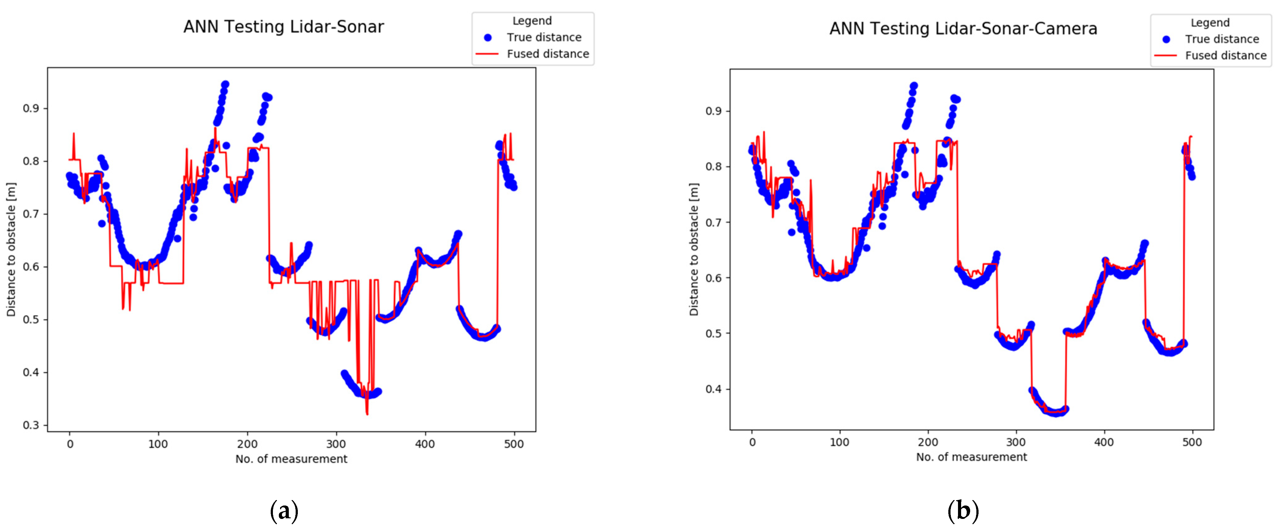
| Train Dataset | 0.03289 m | 0.026143 m |
| Test Dataset | 0.03567 m | 0.029696 m |
| LiDAR Dataset | 2.12175 m | 2.121759 m |
Publisher’s Note: MDPI stays neutral with regard to jurisdictional claims in published maps and institutional affiliations. |
© 2021 by the authors. Licensee MDPI, Basel, Switzerland. This article is an open access article distributed under the terms and conditions of the Creative Commons Attribution (CC BY) license (https://creativecommons.org/licenses/by/4.0/).
Share and Cite
Barreto-Cubero, A.J.; Gómez-Espinosa, A.; Escobedo Cabello, J.A.; Cuan-Urquizo, E.; Cruz-Ramírez, S.R. Sensor Data Fusion for a Mobile Robot Using Neural Networks. Sensors 2022, 22, 305. https://doi.org/10.3390/s22010305
Barreto-Cubero AJ, Gómez-Espinosa A, Escobedo Cabello JA, Cuan-Urquizo E, Cruz-Ramírez SR. Sensor Data Fusion for a Mobile Robot Using Neural Networks. Sensors. 2022; 22(1):305. https://doi.org/10.3390/s22010305
Chicago/Turabian StyleBarreto-Cubero, Andres J., Alfonso Gómez-Espinosa, Jesús Arturo Escobedo Cabello, Enrique Cuan-Urquizo, and Sergio R. Cruz-Ramírez. 2022. "Sensor Data Fusion for a Mobile Robot Using Neural Networks" Sensors 22, no. 1: 305. https://doi.org/10.3390/s22010305