
A Comparison of Three Airborne Laser Scanner Types for Species Identification of Individual Trees

 and
and
Abstract
:1. Introduction
2. Materials
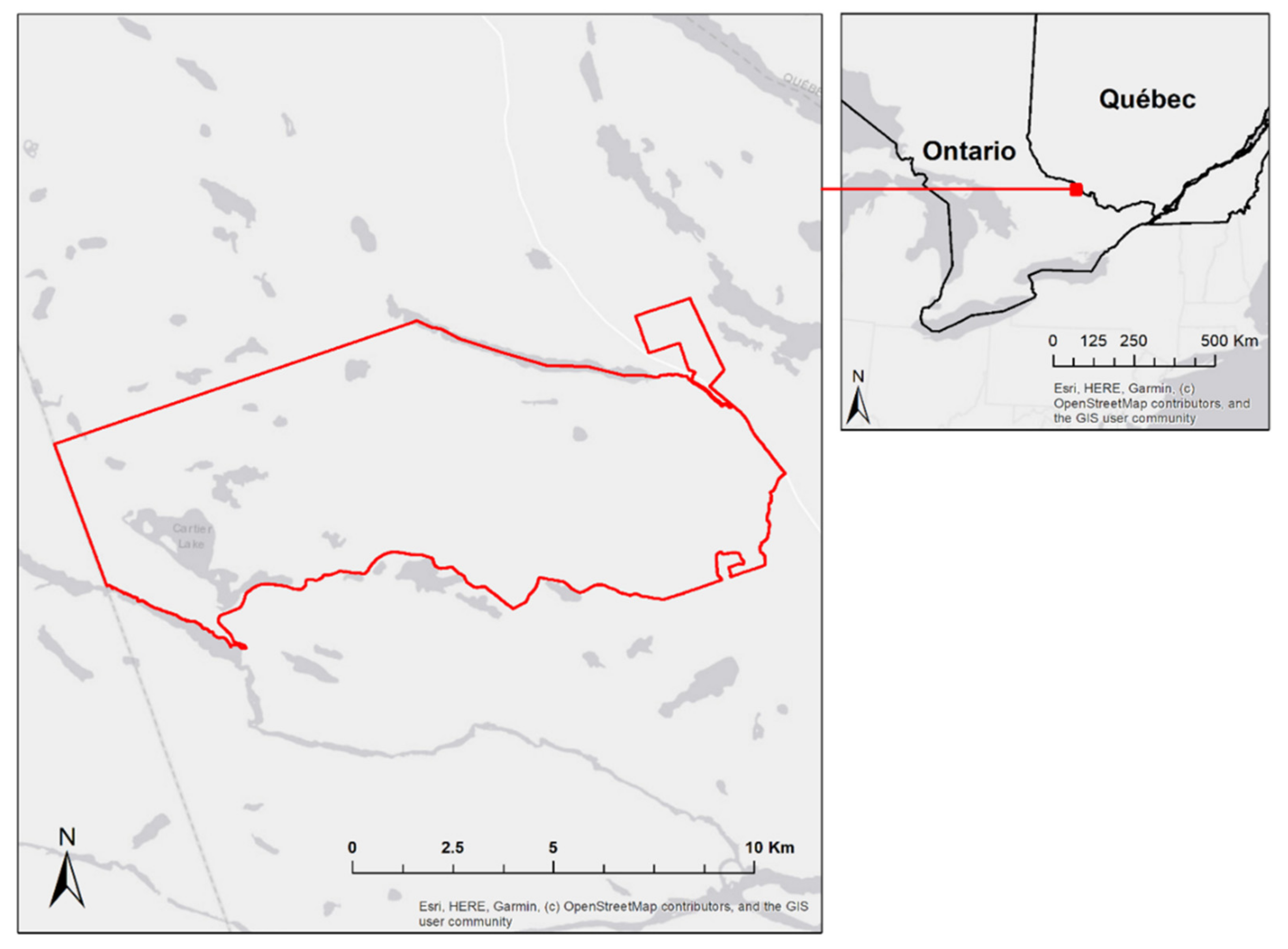
2.1. Study Area
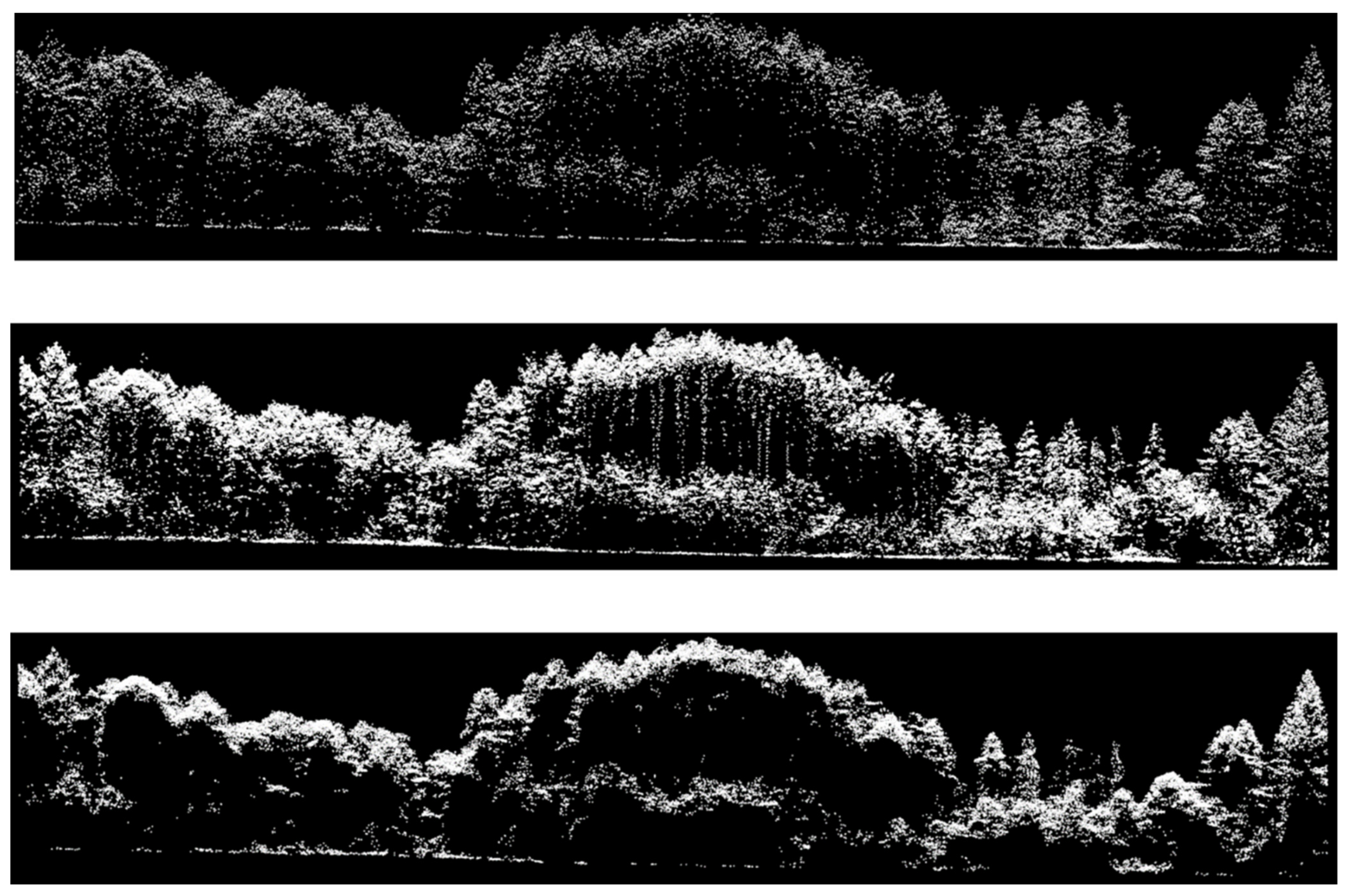
2.2. Airborne Laser Scanning Data
3. Methods
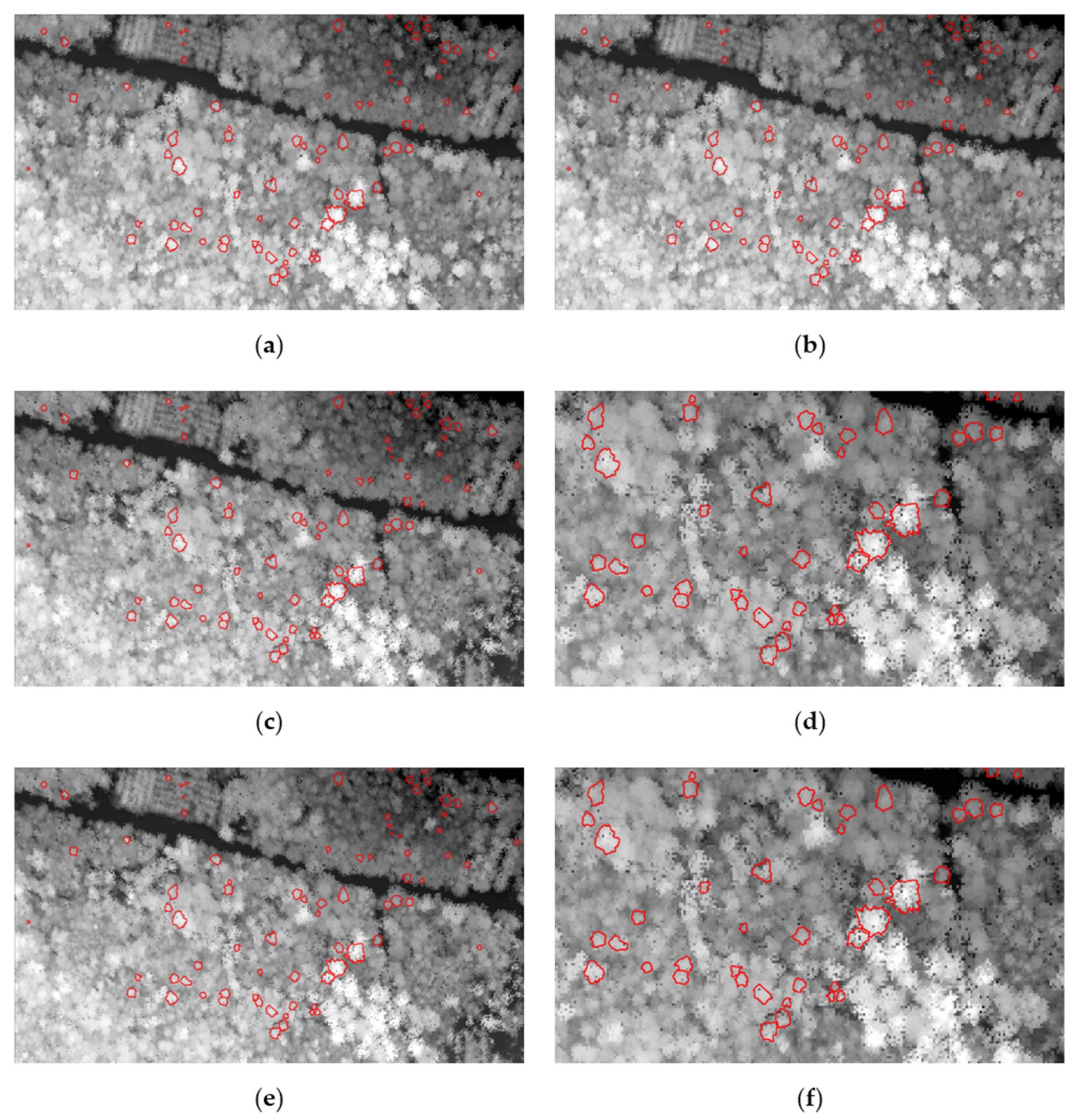
3.1. Individual Tree Crown (ITC) Segmentation
3.2. Feature Calculation
3.3. Species Classification Model
3.3.1. Training Crown Selection
3.3.2. Classification Groupings
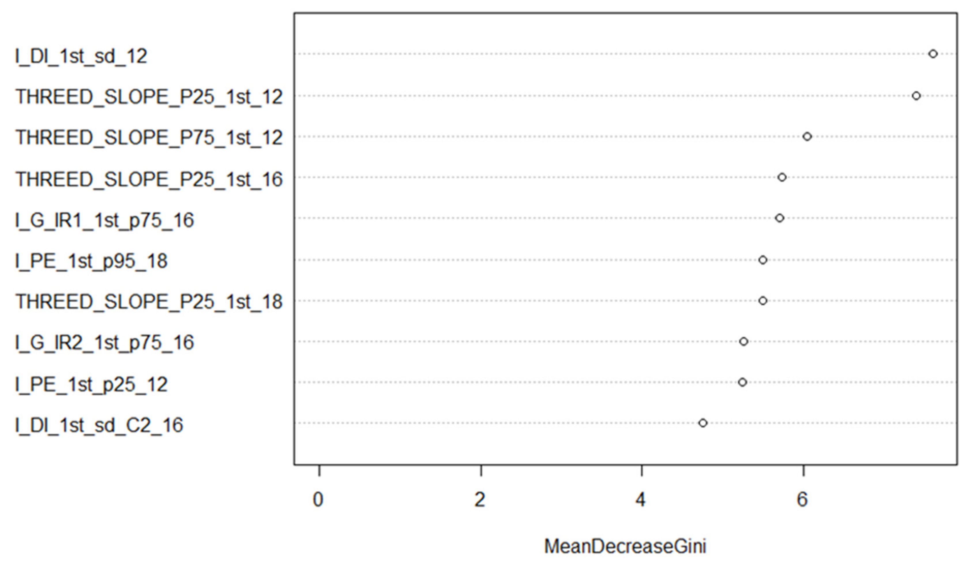
3.3.3. Random Forest Training and Feature Selection
4. Results
5. Discussion
5.1. Factors Influencing Tree Identification Accuracy
5.2. Implications for Forest Inventory
5.3. Limitations and Research Avenues
6. Conclusions
Author Contributions
Funding
Institutional Review Board Statement
Informed Consent Statement
Data Availability Statement
Acknowledgments
Conflicts of Interest
References
- Xu, C.; Morgenroth, J.; Manley, B. Integrating Data from Discrete Return Airborne LiDAR and Optical Sensors to Enhance the Accuracy of Forest Description: A Review. Curr. For. Rep. 2015, 1, 206–219. [Google Scholar] [CrossRef] [Green Version]
- Cao, L.; Coops, N.C.; Hermosilla, T.; Innes, J.L.; Dai, J.; She, G. Using Small-Footprint Discrete and Full-Waveform Airborne LiDAR Metrics to Estimate Total Biomass and Biomass Components in Subtropical Forests. Remote Sens. 2014, 6, 7110–7135. [Google Scholar] [CrossRef] [Green Version]
- Felbermeier, B.; Hahn, A.; Schneider, T.; München, T.U.; Management, F. Study on User Requirements for Remote Sensing Applications in Forestry. In Proceedings of the ISPRS TC VII Symposium—100 Years ISPRS, Vienna, Austria, 5–7 July 2010; Wagner, W., Székely, B., Eds.; IAPRS: Vienna, Austria, 2010; Volume XXXVIII, pp. 210–212. [Google Scholar]
- Shang, X.; Chisholm, L.A. Classification of Australian native forest species using hyperspectral remote sensing and machine-learning classification algorithms. IEEE J. Sel. Top. Appl. Earth Obs. Remote Sens. 2014, 7, 2481–2489. [Google Scholar] [CrossRef]
- Vastaranta, M.; Saarinen, N.; Kankare, V.; Holopainen, M.; Kaartinen, H.; Hyyppä, J.; Hyyppä, H. Multisource single-tree inventory in the prediction of tree quality variables and logging recoveries. Remote Sens. 2014, 6, 3475–3491. [Google Scholar] [CrossRef] [Green Version]
- Yu, X.; Hyyppä, J.; Litkey, P.; Kaartinen, H.; Vastaranta, M.; Holopainen, M. Single-Sensor Solution to Tree Species Classification Using Multispectral Airborne Laser Scanning. Remote Sens. 2017, 9, 108. [Google Scholar] [CrossRef] [Green Version]
- Holopainen, M.; Vastaranta, M.; Hyyppä, J. Outlook for the next generation’s precision forestry in Finland. Forests 2014, 5, 1682–1694. [Google Scholar] [CrossRef] [Green Version]
- White, J.C.; Coops, N.C.; Wulder, M.A.; Vastaranta, M.; Hilker, T.; Tompalski, P. Remote Sensing Technologies for Enhancing Forest Inventories: A Review. Can. J. Remote Sens. 2016, 42, 619–641. [Google Scholar] [CrossRef] [Green Version]
- White, J.C.; Wulder, M.A.; Varhola, A.; Vastaranta, M.; Coops, N.C.; Cook, B.D.; Pitt, D.; Woods, M. A best practices guide for generating forest inventory attributes from airborne laser scanning data using an area-based approach. For. Chron. 2013, 89, 722–723. [Google Scholar] [CrossRef] [Green Version]
- Yu, Q.; Gong, P.; Clinton, N.; Biging, G.; Kelly, M.; Schirokauer, D. Object-based detailed vegetation classification with airborne high spatial resolution remote sensing imagery. Photogramm. Eng. Remote Sens. 2006, 72, 799–811. [Google Scholar] [CrossRef] [Green Version]
- Fassnacht, F.E.; Latifi, H.; Stereńczak, K.; Modzelewska, A.; Lefsky, M.A.; Waser, L.T.; Straub, C.; Ghosh, A. Review of studies on tree species classification from remotely sensed data. Remote Sens. Environ. 2016, 186, 64–87. [Google Scholar] [CrossRef]
- Van Aardt, J.A.N.; Wynne, R.H. Examining pine spectral separability using hyperspectral data from an airborne sensor: An extension of field-based results. Int. J. Remote Sens. 2007, 28, 431–436. [Google Scholar] [CrossRef]
- Pant, P.; Heikkinen, V.; Hovi, A.; Korpela, I.; Hauta-Kasari, M.; Tokola, T. Evaluation of simulated bands in airborne optical sensors for tree species identification. Remote Sens. Environ. 2013, 138, 27–37. [Google Scholar] [CrossRef]
- Schaepman-Strub, G.; Schaepman, M.E.; Painter, T.H.; Dangel, S.; Martonchik, J.V. Reflectance quantities in optical remote sensing—definitions and case studies. Remote Sens. Environ. 2006, 103, 27–42. [Google Scholar] [CrossRef]
- Fassnacht, F.E.; Koch, B. Review of forestry oriented multi-angular remote sensing techniques. Int. For. Rev. 2012, 14, 285–298. [Google Scholar] [CrossRef]
- Leitold, V.; Keller, M.; Morton, D.C.; Cook, B.D.; Shimabukuro, Y.E. Airborne lidar-based estimates of tropical forest structure in complex terrain: Opportunities and trade-offs for REDD+. Carbon Balance Manag. 2015, 10, 3. [Google Scholar] [CrossRef] [PubMed]
- Stoker, J.M.; Abdullah, Q.A.; Nayegandhi, A.; Winehouse, J. Evaluation of single photon and Geiger mode lidar for the 3D Elevation Program. Remote Sens. 2016, 8, 767. [Google Scholar] [CrossRef] [Green Version]
- Woodhouse, I.H.; Nichol, C.; Sinclair, P.; Jack, J.; Morsdorf, F.; Malthus, T.J.; Patenaude, G. A multispectral canopy LiDAR demonstrator project. IEEE Geosci. Remote Sens. Lett. 2011, 8, 839–843. [Google Scholar] [CrossRef]
- Coops, N.C.; Hilker, T.; Wulder, M.A.; St-Onge, B.; Newnham, G.; Siggins, A.; Trofymow, J.A. Estimating canopy structure of Douglas-fir forest stands from discrete-return LiDAR. Trees-Struct. Funct. 2007, 21, 295–310. [Google Scholar] [CrossRef] [Green Version]
- Suratno, A.; Seielstad, C.; Queen, L. Tree species identification in mixed coniferous forest using airborne laser scanning. ISPRS J. Photogramm. Remote Sens. 2009, 64, 683–693. [Google Scholar] [CrossRef]
- Kim, S.; McGaughey, R.J.; Andersen, H.E.; Schreuder, G. Tree species differentiation using intensity data derived from leaf-on and leaf-off airborne laser scanner data. Remote Sens. Environ. 2009, 113, 1575–1586. [Google Scholar] [CrossRef]
- Korpela, I.; Ørka, H.O.; Maltamo, M.; Tokola, T.; Hyyppä, J. Tree species classification using airborne LiDAR—Effects of stand and tree parameters, downsizing of training set, intensity normalization, and sensor type. Silva Fenn. 2010, 44, 319–339. [Google Scholar] [CrossRef] [Green Version]
- Fernandez-Diaz, J.; Carter, W.; Glennie, C.; Shrestha, R.; Pan, Z.; Ekhtari, N.; Singhania, A.; Hauser, D.; Sartori, M. Capability Assessment and Performance Metrics for the Titan Multispectral Mapping Lidar. Remote Sens. 2016, 8, 936. [Google Scholar] [CrossRef] [Green Version]
- Næsset, E.; Gobakken, T.; Holmgren, J.; Hyyppä, H.; Hyyppä, J.; Maltamo, M.; Nilsson, M.; Olsson, H.; Persson, Å.; Söderman, U. Laser scanning of forest resources: The nordic experience. Scand. J. For. Res. 2004, 19, 482–499. [Google Scholar] [CrossRef]
- Priedhorsky, W.C.; Smith, R.C.; Ho, C. Laser ranging and mapping with a photon-counting detector. Appl. Opt. 1996, 35, 441–452. [Google Scholar] [CrossRef]
- Li, Q.; Degnan, J.; Barrett, T.; Shan, J. First Evaluation on Single Photon-Sensitive Lidar Data. Photogramm. Eng. Remote Sens. 2016, 82, 455–463. [Google Scholar] [CrossRef]
- Swatantran, A.; Tang, H.; Barrett, T.; Decola, P.; Dubayah, R. Rapid, high-resolution forest structure and terrain mapping over large areas using single photon lidar. Sci. Rep. 2016, 6, 1–12. [Google Scholar] [CrossRef] [Green Version]
- Degnan, J.; Machan, R.; Leventhal, E.; Lawrence, D.; Jodor, G.; Field, C. Inflight performance of a second-generation photon-counting 3D imaging lidar. In Laser Radar Technology and Applications XIII; International Society for Optics and Photonics: Bellingham, WA, USA, 2008; Volume 6950, p. 695007. [Google Scholar]
- Shrestha, K.Y.; Carter, W.E.; Slatton, K.C.; Cossio, T.K. Shallow bathymetric mapping via multistop single photoelectron sensitivity laser ranging. IEEE Trans. Geosci. Remote Sens. 2012, 50, 4771–4790. [Google Scholar] [CrossRef]
- Harding, D. Pulsed laser altimeter ranging techniques and implications for terrain mapping. In Topographic Laser Ranging and Scanning: Principles and Processing; Shan, J., Toth, C., Eds.; CRC Press: Boca Raton, FL, USA, 2018; pp. 173–194. [Google Scholar]
- Degnan, J.J. Scanning, multibeam, single photon lidars for rapid, large scale, high resolution, topographic and bathymetric mapping. Remote Sens. 2016, 8, 958. [Google Scholar] [CrossRef] [Green Version]
- Yu, X.; Kukko, A.; Kaartinen, H.; Wang, Y.; Liang, X.; Matikainen, L.; Hyyppä, J. Comparing features of single and multi-photon lidar in boreal forests. ISPRS J. Photogramm. Remote Sens. 2020, 168, 268–276. [Google Scholar] [CrossRef]
- White, J.C.; Penner, M.; Woods, M. Assessing single photon LiDAR for operational implementation of an enhanced forest inventory in diverse mixedwood forests. For. Chron. 2021, 97, 78–96. [Google Scholar] [CrossRef]
- Wästlund, A.; Holmgren, J.; Lindberg, E.; Olsson, H. Forest Variable Estimation Using a High Altitude Single Photon Lidar System. Remote Sens. 2018, 10, 1422. [Google Scholar] [CrossRef] [Green Version]
- Rowe, J.S. Forest Regions of Canada; Information Canada: Ottawa, ON, Canada, 1972; ISBN Fo47-1300. [Google Scholar]
- Environment Canada Canadian Climate Normals 1981–2010. Available online: http://climate.weather.gc.ca/climate_normals/index_e.html (accessed on 13 August 2019).
- Woods, M.; Lim, K.; Treitz, P. Predicting forest stand variables from LiDAR data in the Great Lakes—St. Lawrence forest of Ontario. For. Chron. 2008, 84, 827–839. [Google Scholar] [CrossRef] [Green Version]
- Budei, B.C.; St-Onge, B.; Hopkinson, C.; Audet, F.-A. Identifying the genus or species of individual trees using a three-wavelength airborne lidar system. Remote Sens. Environ. 2018, 204, 632–647. [Google Scholar] [CrossRef]
- Breiman, L. Random forests. Mach. Learn. 2001, 45, 5–32. [Google Scholar] [CrossRef] [Green Version]
- Georganos, S.; Grippa, T.; Vanhuysse, S.; Lennert, M.; Shimoni, M.; Kalogirou, S.; Wolff, E. Less is more: Optimizing classification performance through feature selection in a very-high-resolution remote sensing object-based urban application. GIScience Remote Sens. 2018, 55, 221–242. [Google Scholar] [CrossRef]
- Lindsay, J.B. Whitebox GAT: A case study in geomorphometric analysis. Comput. Geosci. 2016, 95, 75–84. [Google Scholar] [CrossRef]
- Sadeghi, Y.; St-Onge, B.; Leblon, B.; Simard, M. Canopy Height Model (CHM) Derived from a TanDEM-X InSAR DSM and an Airborne Lidar DTM in Boreal Forest. IEEE J. Sel. Top. Appl. Earth Obs. Remote Sens. 2016, 9, 381–397. [Google Scholar] [CrossRef]
- Vega, C.; Hamrouni, A.; El Mokhtari, A.; Morel, M.; Bock, J.; Renaud, J.P.; Bouvier, M.; Durrieue, S. PTrees: A point-based approach to forest tree extractionfrom lidar data. Int. J. Appl. Earth Obs. Geoinf. 2014, 33, 98–108. [Google Scholar] [CrossRef]
- Budei, B.C.; St-Onge, B. Variability of Multispectral Lidar 3D and Intensity Features with Individual Tree Height and Its Influence on Needleleaf Tree Species Identification. Can. J. Remote Sens. 2018, 263-286, 263–286. [Google Scholar] [CrossRef]
- Okhrimenko, M.; Coburn, C.; Hopkinson, C. Multi-spectral lidar: Radiometric calibration, canopy spectral reflectance, and vegetation vertical SVI profiles. Remote Sens. 2019, 11, 1556. [Google Scholar] [CrossRef] [Green Version]
- Brown, R.; Hartzell, P.; Glennie, C. Evaluation of SPL100 single photon lidar data. Remote Sens. 2020, 12, 722. [Google Scholar] [CrossRef] [Green Version]
- Fernandez-Delgado, M.; Cernadas, E.; Barro, S. Do we Need Hundreds of Classifiers to Solve Real World Classification Problems? J. Mach. Learn. 2014, 15, 3133–3181. [Google Scholar]
- Ørka, H.O.; Dalponte, M.; Gobakken, T.; Næsset, E.; Ene, L.T. Characterizing forest species composition using multiple remote sensing data sources and inventory approaches. Scand. J. For. Res. 2013, 28, 677–688. [Google Scholar] [CrossRef]
- Immitzer, M.; Atzberger, C.; Koukal, T. Tree species classification with Random forest using very high spatial resolution 8-band worldView-2 satellite data. Remote Sens. 2012, 4, 2661–2693. [Google Scholar] [CrossRef] [Green Version]
- Chen, C.; Liaw, A.; Breiman, L. Using Random Forest to Learn Imbalanced Data. Available online: http://statistics.berkeley.edu/sites/default/files/tech-reports/666.pdf (accessed on 15 August 2019).
- Hughes, G.F. On the Mean Accuracy of Statistical Pattern Recognizers. IEEE Trans. Inf. Theory 1968, 14, 55–63. [Google Scholar] [CrossRef] [Green Version]
- Guyon, I.; Elisseeff, A. An introduction to variable and feature selection. J. Mach. Learn. Res. 2003, 3, 1157–1182. [Google Scholar]
- Liaw, A.; Wiener, M. Classification and Regression by randomForest. R News 2002, 2, 18–22. [Google Scholar]
- R Core Team. R: A Language and Environment for Statistical Computing; R Foundation for Statistical Computing: Vienna, Austria, 2019; Available online: http://www.R-project.org/ (accessed on 24 September 2019).
- Genuer, R.; Poggi, J.M.; Tuleau-Malot, C. VSURF: An R package for variable selection using random forests. R J. 2015, 7, 19–33. [Google Scholar] [CrossRef] [Green Version]
- Axelsson, A.; Lindberg, E.; Olsson, H. Exploring multispectral ALS data for tree species classification. Remote Sens. 2018, 10, 183. [Google Scholar] [CrossRef] [Green Version]
- Hartzell, P.; Dang, Z.; Pan, Z.; Glennie, C. Radiometric evaluation of an airborne single photon LiDAR sensor. IEEE Geosci. Remote Sens. Lett. 2018, 15, 1466–1470. [Google Scholar] [CrossRef]
- Jones, T.G.; Coops, N.C.; Sharma, T. Assessing the utility of airborne hyperspectral and LiDAR data for species distribution mapping in the coastal Pacific Northwest, Canada. Remote Sens. Environ. 2010, 114, 2841–2852. [Google Scholar] [CrossRef]
- Sasaki, T.; Imanishi, J.; Ioki, K.; Morimoto, Y.; Kitada, K. Object-based classification of land cover and tree species by integrating airborne LiDAR and high spatial resolution imagery data. Landsc. Ecol. Eng. 2012, 8, 157–171. [Google Scholar] [CrossRef]
- Zhang, C.; Qiu, F. Mapping Individual Tree Species in an Urban Forest Using Airborne Lidar Data and Hyperspectral Imagery. Photogramm. Eng. Remote Sens. 2012, 78, 1079–1087. [Google Scholar] [CrossRef] [Green Version]
- White, J.C.; Woods, M. Exploring the Innovation Potential of Single Photon Lidar for Ontario’s eFRI: Final Report to the Ontario Forestry Futures Trust; Ontario Forestry Futures Trust: Thunder Bay, ON, Canada, 2018. [Google Scholar]
- Naidoo, L.; Cho, M.A.; Mathieu, R.; Asner, G. Classification of savanna tree species, in the Greater Kruger National Park region, by integrating hyperspectral and LiDAR data in a Random Forest data mining environment. ISPRS J. Photogramm. Remote Sens. 2012, 69, 167–179. [Google Scholar] [CrossRef]
- Packalen, P.; Suvanto, A.; Maltamo, M. A two stage method to estimate species-specific growing stock. Photogramm. Eng. Remote Sens. 2009, 75, 1451–1460. [Google Scholar] [CrossRef]
- Puttonen, E.; Suomalainen, J.; Hakala, T.; Räikkönen, E.; Kaartinen, H.; Kaasalainen, S.; Litkey, P. Tree species classification from fused active hyperspectral reflectance and LIDAR measurements. For. Ecol. Manag. 2010, 260, 1843–1852. [Google Scholar] [CrossRef]
- White, J.C.; Woods, M.; Krahn, T.; Papasodoro, C.; Bélanger, D.; Onafrychuk, C.; Sinclair, I. Evaluating the capacity of single photon lidar for terrain characterization under a range of forest conditions. Remote Sens. Environ. 2021, 252, 112169. [Google Scholar] [CrossRef]
- Foody, G.M.; Mathur, A. Toward intelligent training of supervised image classifications: Directing training data acquisition for SVM classification. Remote Sens. Environ. 2004, 93, 107–117. [Google Scholar] [CrossRef]
- Kim, S.Y. Effects of sample size on robustness and prediction accuracy of a prognostic gene signature. BMC Bioinform. 2009, 10, 4–7. [Google Scholar] [CrossRef] [PubMed] [Green Version]
- Millard, K.; Richardson, M. On the importance of training data sample selection in Random Forest image classification: A case study in peatland ecosystem mapping. Remote Sens. 2015, 7, 8489–8515. [Google Scholar] [CrossRef] [Green Version]
- LeCun, Y.; Bengio, Y.; Hinton, G. Deep learning. Nature 2015, 521, 436–444. [Google Scholar] [CrossRef]
- Frénay, B.; Verleysen, M. Classification in the presence of label noise: A survey. IEEE Trans. Neural Netw. Learn. Syst. 2014, 25, 845–869. [Google Scholar] [CrossRef] [PubMed]
- Pelletier, C.; Valero, S.; Inglada, J.; Champion, N.; Sicre, C.M.; Dedieu, G. Effect of training class label noise on classification performances for land cover mapping with satellite image time series. Remote Sens. 2017, 9, 173. [Google Scholar] [CrossRef] [Green Version]
- Maas, A.; Rottensteiner, F.; Heipke, C. Using Label Noise Robust Logistic Regression for Automated Updating of Topographic Geospatial Databases. ISPRS Ann. Photogramm. Remote Sens. Spat. Inf. Sci. 2016, 3, 133–140. [Google Scholar] [CrossRef] [Green Version]


| Parameter | ALS12 | MSL16 | SPL18 |
|---|---|---|---|
| Acquisition date | 17–20 August 2012 | 20 July 2016 | 1–2 July 2018 |
| Sensor | Riegl 680i | Optech Titan | Leica SPL100 |
| Laser wavelength (nm) | 1550 | 532/1064/1550 | 532 |
| Laser beam divergence (mrad) | 0.5 | 0.7/0.7/0.35 | 0.08 |
| Avg. flying altitude (m AGL) | 750 | 600 | 3760 |
| Avg. flying speed (kts) | <100 | <140 | <180 |
| Pulse repetition frequency (kHz) | 150 | 375 (3 channels) | 60 |
| Frequency (Hz) | 76.67 | 40 | 23 |
| Scan angle (degrees) | ±20 | ±35 | ±15 |
| Field-of-View (degrees) | 40 | 30 | 30 |
| Aggregate point density (points/m2) | 5.8 | 4.8/12.4/11.9 ~30 (combined) | 28.6 |
| Symbol | Description | Return Types | Statistics |
|---|---|---|---|
| DI | Dispersion (coefficient of variation of return heights) | all, 1st | cv |
| SLOPE | Slope of the lines connecting the highest return to each of the other returns | all, 1st | mn, sd, cv, p25, p50, p75 |
| RB | Ratio of the number of returns in different height bins (% of height) over total number of returns | all | Counts: 60_80, 80_90, 90_100, 95_100 |
| CH | Ratio of the convex hull volume over maximum height cubed | all | N/A |
| RM | Ratio between different statistics and different types of return | all, 1st, 2nd | mn, p50 |
| Symbol | Description | Return Types | Statistics |
|---|---|---|---|
| DI | Dispersion (coefficient of variation of intensity) | 1st | sd, cv |
| PE | Intensity values at given height percentiles | 1st | p5, p10, p25, p50, p75, p90, p95 |
| MI | Mean intensity of returns between interval of percentiles | 1st | mn: all, p5_95, p10_90, |
| RM | Ratio between different statistics | all, 1st, 2nd | mn, p50 |
| G_IR1 (MSL) | Type 1 Green Normalised Difference Vegetation Index (532 nm and 1064) | 1st | mn, p50, p75 |
| G_IR2 (MSL) | Type 2 Green Normalised Difference Vegetation Index (532 nm and 1550 nm) | 1st | mn, p50, p75 |
| NDIR (MSL) | IR Normalised Difference Vegetation Index (1064 nm and 1550 nm) | 1st | mn, p50, p75 |
| Simple ratios of 3 MSL wavelengths | 1st | mn, p50, p75 |
| Species | n |
|---|---|
| Black ash | 45 |
| White ash | 40 |
| Basswood | 56 |
| Beech | 70 |
| Balsam fir | 78 |
| Paper birch | 53 |
| Yellow birch | 40 |
| Eastern white cedar | 44 |
| Eastern larch | 46 |
| Sugar maple | 137 |
| Red maple | 54 |
| Red oak | 72 |
| Jack pine | 89 |
| Bigtooth aspen | 100 |
| Red pine | 109 |
| Trembling aspen | 48 |
| White pine | 159 |
| Black spruce | 65 |
| White spruce | 108 |
| HW/SW | ALS12 | MSL16 | SPL18 |
|---|---|---|---|
| Hardwood | 683 | 614 | 596 |
| Softwood | 673 | 566 | 546 |
| Four Genera | |||
| Acer (maple) | 185 | 175 | 155 |
| Pinus (pine) | 345 | 280 | 302 |
| Populus (poplar) | 135 | 102 | 139 |
| Picea (spruce) | 171 | 154 | 130 |
| Functional Group (Fct. Gr.) | |||
| Hardwood | 308 | 297 | 262 |
| Intolerant hardwood | 375 | 317 | 334 |
| Other softwood | 157 | 132 | 114 |
| Pine | 345 | 280 | 302 |
| Spruce | 171 | 154 | 130 |
| 12 Species | |||
| Ash (Black/White) (AS) | 81 | 70 | 66 |
| Basswood (BA) | 56 | 53 | 48 |
| American Beech (BE) | 67 | 69 | 59 |
| Birch (Paper/Yellow) (BI) | 89 | 80 | 77 |
| Eastern White Cedar (CE) | 44 | 43 | 36 |
| Balsam Fir (BF) | 69 | 53 | 43 |
| Eastern Larch (LA) | 44 | 36 | 35 |
| Maple (Red/Sugar) (MA) | 185 | 175 | 155 |
| Red Oak (OK) | 70 | 65 | 52 |
| Pine (Red/White) (PI) | 345 | 280 | 302 |
| Trembling Aspen (PO) | 135 | 102 | 139 |
| Spruce (Black/White) (SP) | 171 | 254 | 130 |
| ALS12 | MSL16 | SPL18 | ALL ALS | |||||||
|---|---|---|---|---|---|---|---|---|---|---|
| 3D | I | All | 3D | I | All | 3D | I | All | All | |
| Type (HW/SW) | ||||||||||
| All features | 84.0 | 76.2 | 86.4 | 82.9 | 85.2 | 90.4 | 80.1 | 59.1 | 82.9 | 90.3 |
| 25 features | N/A | N/A | 86.1 | N/A | 85.2 | 90.4 | N/A | N/A | N/A | 91.1 |
| 15 features | 84.1 | N/A | 86.3 | 82.9 | 85.0 | 89.9 | 80.1 | N/A | 82.7 | 91.0 |
| 4 genera | ||||||||||
| All features | 65.4 | 64.7 | 75.1 | 67.8 | 71.7 | 78.6 | 64.5 | 50.1 | 68.3 | 83.4 |
| 25 features | 65.5 | N/A | 74.3 | N/A | 71.8 | 78.1 | N/A | N/A | N/A | 83.5 |
| 15 features | 63.6 | N/A | 74.2 | 66.4 | 71.8 | 76.8 | 63.5 | N/A | 68.1 | 81.4 |
| Functional Group | ||||||||||
| All features | 55.7 | 52.5 | 68.9 | 54.3 | 64.1 | 69.6 | 50.4 | 43.3 | 63.6 | 75.0 |
| 25 features | N/A | N/A | 67.4 | N/A | 64.3 | 69.2 | N/A | N/A | N/A | 73.0 |
| 15 features | 55.3 | N/A | 66.2 | 54.1 | 64.1 | 68.6 | 50.0 | N/A | 64.4 | 72.5 |
| 12 species | ||||||||||
| All features | 38.9 | 33.2 | 50.7 | 36.8 | 48.2 | 53.2 | 37.8 | 25.8 | 44.5 | 58.0 |
| 25 features | N/A | N/A | 51.3 | N/A | 48.5 | 53.5 | N/A | N/A | N/A | 57.0 |
| 15 features | 38.3 | N/A | 48.7 | 37.3 | 47.5 | 51.5 | 38.4 | N/A | 44.8 | 54.2 |
| AS | BA | BE | BI | CE | BF | LA | MA | OK | PI | PO | SP | OOB Accuracy % | |
| AS | 22 | 4 | 1 | 5 | 0 | 0 | 1 | 5 | 9 | 4 | 4 | 1 | 39 |
| BA | 10 | 13 | 3 | 2 | 0 | 0 | 1 | 3 | 4 | 5 | 4 | 1 | 28 |
| BE | 1 | 0 | 36 | 2 | 0 | 0 | 0 | 14 | 0 | 0 | 2 | 1 | 64 |
| BI | 7 | 1 | 4 | 21 | 3 | 0 | 0 | 6 | 9 | 5 | 10 | 1 | 31 |
| CE | 4 | 1 | 0 | 1 | 26 | 0 | 1 | 0 | 0 | 0 | 0 | 3 | 72 |
| BF | 0 | 1 | 1 | 0 | 2 | 22 | 1 | 0 | 2 | 0 | 0 | 5 | 65 |
| LA | 0 | 0 | 0 | 0 | 4 | 0 | 10 | 0 | 0 | 4 | 0 | 11 | 35 |
| MA | 4 | 5 | 28 | 5 | 1 | 1 | 0 | 81 | 2 | 7 | 10 | 2 | 56 |
| OK | 5 | 2 | 0 | 3 | 0 | 0 | 0 | 2 | 31 | 1 | 2 | 1 | 66 |
| PI | 3 | 6 | 0 | 1 | 13 | 4 | 10 | 1 | 2 | 185 | 16 | 10 | 74 |
| PO | 11 | 5 | 4 | 10 | 4 | 4 | 1 | 2 | 3 | 6 | 42 | 4 | 44 |
| SP | 0 | 3 | 0 | 0 | 5 | 7 | 3 | 1 | 0 | 7 | 3 | 88 | 75 |
Publisher’s Note: MDPI stays neutral with regard to jurisdictional claims in published maps and institutional affiliations. |
© 2021 by the authors. Licensee MDPI, Basel, Switzerland. This article is an open access article distributed under the terms and conditions of the Creative Commons Attribution (CC BY) license (https://creativecommons.org/licenses/by/4.0/).
Share and Cite
Prieur, J.-F.; St-Onge, B.; Fournier, R.A.; Woods, M.E.; Rana, P.; Kneeshaw, D. A Comparison of Three Airborne Laser Scanner Types for Species Identification of Individual Trees. Sensors 2022, 22, 35. https://doi.org/10.3390/s22010035
Prieur J-F, St-Onge B, Fournier RA, Woods ME, Rana P, Kneeshaw D. A Comparison of Three Airborne Laser Scanner Types for Species Identification of Individual Trees. Sensors. 2022; 22(1):35. https://doi.org/10.3390/s22010035
Chicago/Turabian StylePrieur, Jean-François, Benoît St-Onge, Richard A. Fournier, Murray E. Woods, Parvez Rana, and Daniel Kneeshaw. 2022. "A Comparison of Three Airborne Laser Scanner Types for Species Identification of Individual Trees" Sensors 22, no. 1: 35. https://doi.org/10.3390/s22010035
APA StylePrieur, J.-F., St-Onge, B., Fournier, R. A., Woods, M. E., Rana, P., & Kneeshaw, D. (2022). A Comparison of Three Airborne Laser Scanner Types for Species Identification of Individual Trees. Sensors, 22(1), 35. https://doi.org/10.3390/s22010035