
QADI as a New Method and Alternative to Kappa for Accuracy Assessment of Remote Sensing-Based Image Classification


Abstract
:1. Introduction
2. From Kappa to QADI: The Proposed Approach
2.1. Cohen’s Kappa Coefficient
2.2. Criticisms of Kappa
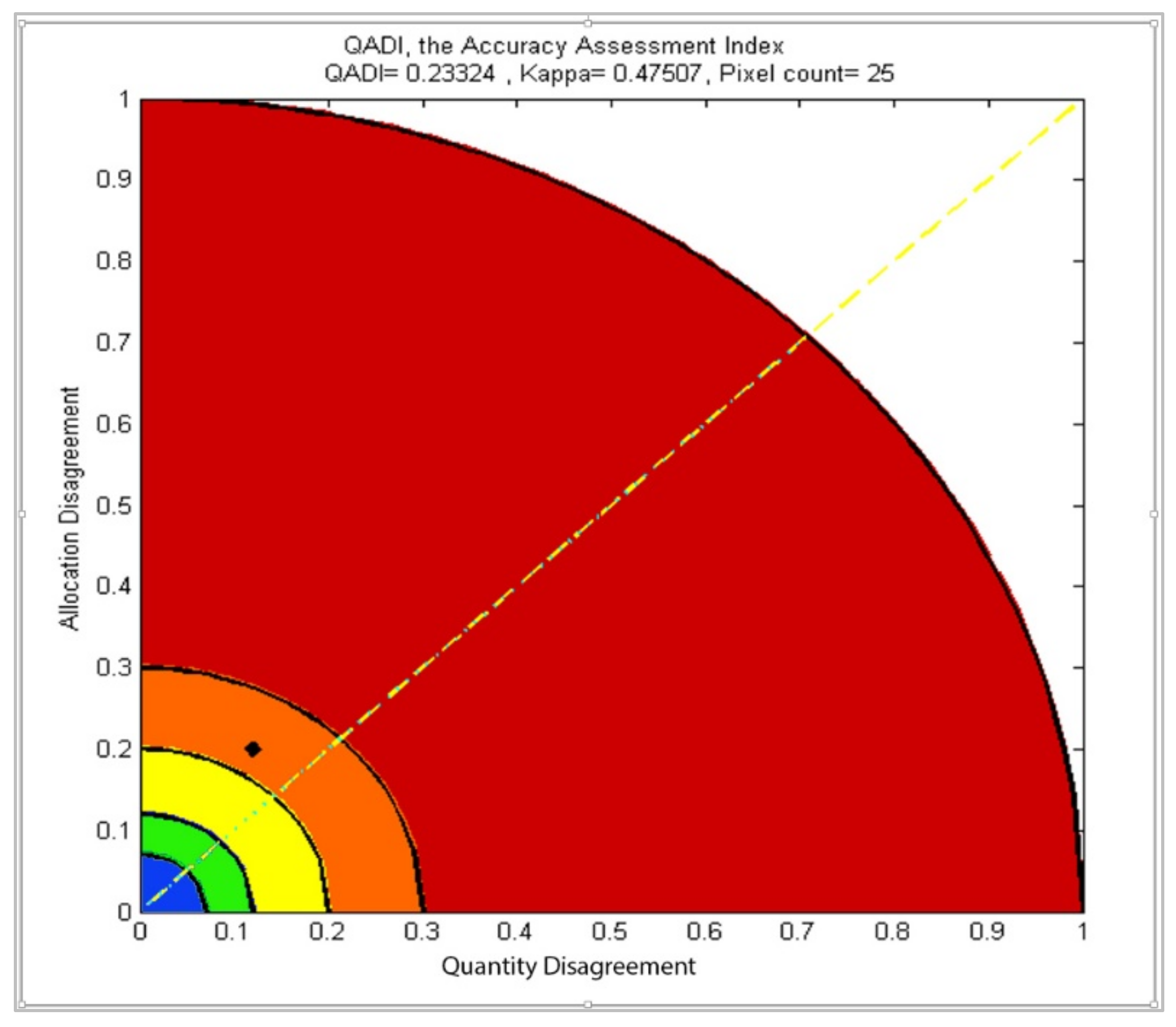
2.3. The Proposed QADI Index for Accuracy Assessment
2.4. The Validation Experiments
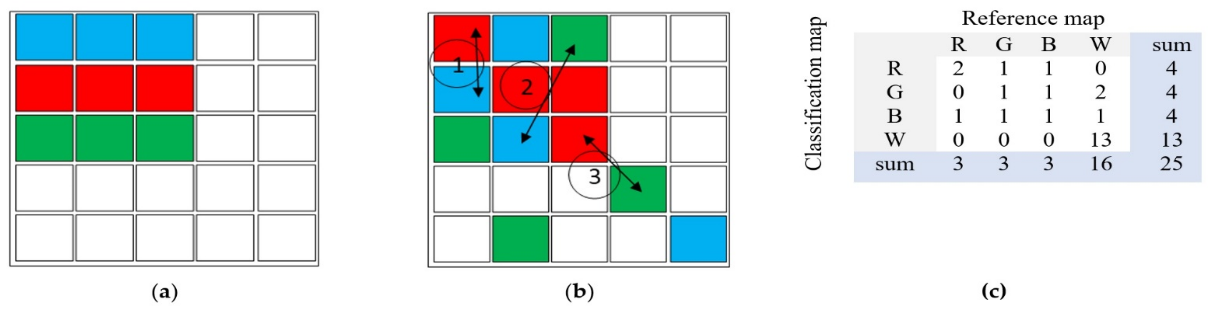
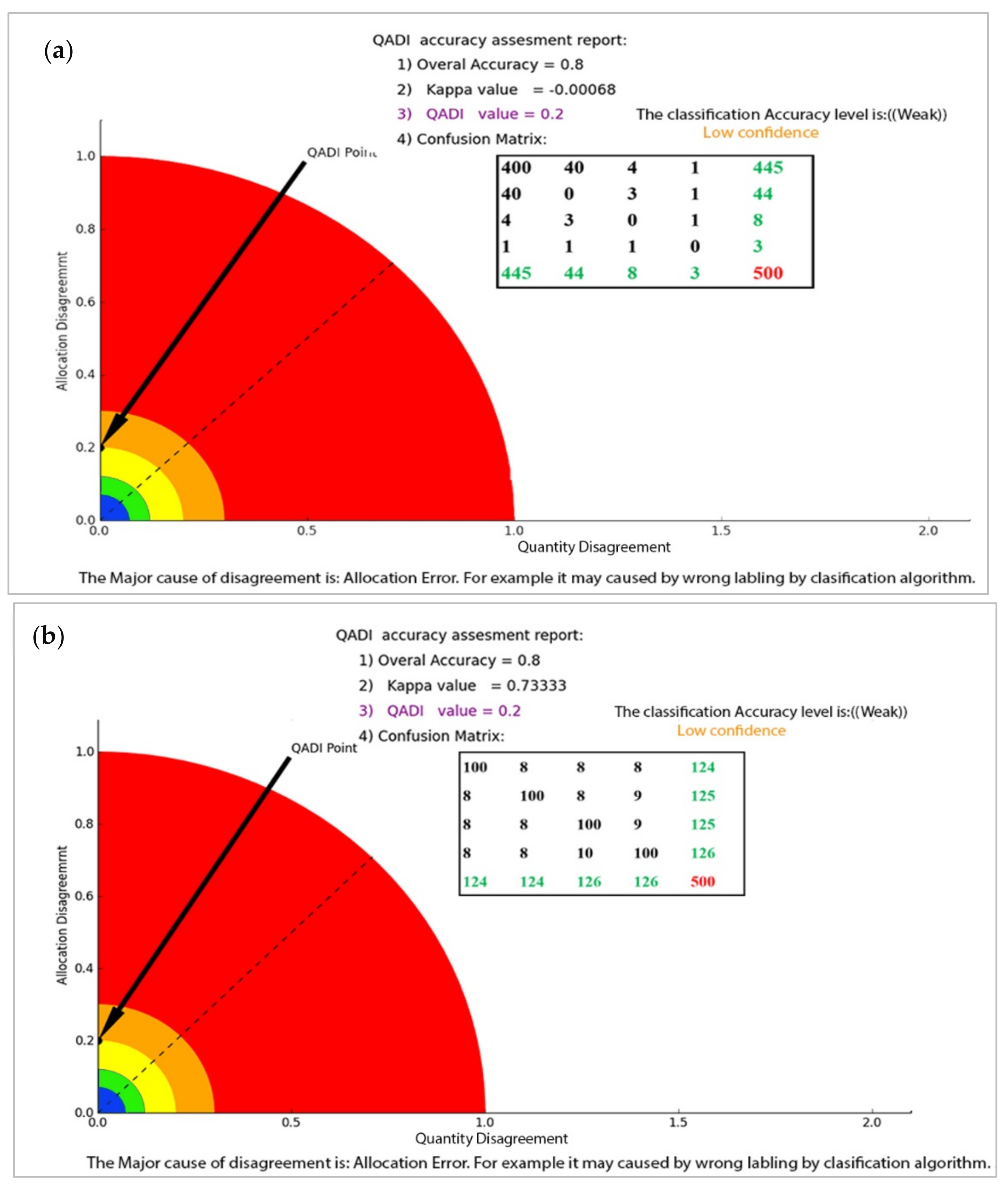
2.5. Confusion Matrix with a Balanced Distribution
2.6. Confusion Matrix with a Skewed Distribution
3. Results
4. Discussion
4.1. Kappa Index and Issues
4.2. Significance of QADI
5. Conclusions
Supplementary Materials
Author Contributions
Funding
Data Availability Statement
Acknowledgments
Conflicts of Interest
References
- Cresson, R. A Framework for Remote Sensing Images Processing Using Deep Learning Techniques. IEEE Geosci. Remote Sens. Lett. 2018, 16, 25–29. [Google Scholar] [CrossRef] [Green Version]
- Sudmanns, M.; Tiede, D.; Lang, S.; Bergstedt, H.; Trost, G.; Augustin, H.; Baraldi, A.; Blaschke, T. Big Earth data: Disruptive changes in Earth observation data management and analysis? Int. J. Digit. Earth 2020, 13, 832–850. [Google Scholar] [CrossRef] [PubMed]
- Chen, Z.; Wagner, M.; Das, J.; Doe, R.; Cerveny, R. Data-Driven Approaches for Tornado Damage Estimation with Unpiloted Aerial Systems. Remote Sens. 2021, 13, 1669. [Google Scholar] [CrossRef]
- Yu, X.; Wu, X.; Luo, C.; Ren, P. Deep learning in remote sensing scene classification: A data augmentation enhanced convolutional neural network framework. GISci. Remote Sens. 2017, 54, 741–758. [Google Scholar] [CrossRef] [Green Version]
- Kussul, N.; Lavreniuk, M.; Skakun, S.; Shelestov, A. Deep Learning Classification of Land Cover and Crop Types Using Remote Sensing Data. IEEE Geosci. Remote Sens. Lett. 2017, 14, 778–782. [Google Scholar] [CrossRef]
- Sharma, A.; Liu, X.; Yang, X.; Shi, D. A patch-based convolutional neural network for remote sensing image classification. Neural Netw. 2017, 95, 19–28. [Google Scholar] [CrossRef]
- Maxwell, A.E.; Warner, T.A.; Fang, F. Implementation of machine-learning classification in remote sensing: An applied review. Int. J. Remote Sens. 2018, 39, 2784–2817. [Google Scholar] [CrossRef] [Green Version]
- Vetrivel, A.; Gerke, M.; Kerle, N.; Nex, F.; Vosselman, G. Disaster damage detection through synergistic use of deep learning and 3D point cloud features derived from very high resolution oblique aerial images, and multiple-kernel-learning. ISPRS J. Photogramm. Remote Sens. 2018, 140, 45–59. [Google Scholar] [CrossRef]
- Talukdar, S.; Singha, P.; Mahato, S.; Shahfahad; Pal, S.; Liou, Y.-A.; Rahman, A. Land-Use Land-Cover Classification by Machine Learning Classifiers for Satellite Observations—A Review. Remote Sens. 2020, 12, 1135. [Google Scholar] [CrossRef] [Green Version]
- Xia, M.; Tian, N.; Zhang, Y.; Xu, Y.; Zhang, X. Dilated multi-scale cascade forest for satellite image classification. Int. J. Remote Sens. 2020, 41, 7779–7800. [Google Scholar] [CrossRef]
- Najafi, P.; Feizizadeh, B.; Navid, H. A Comparative Approach of Fuzzy Object Based Image Analysis and Machine Learning Techniques Which Are Applied to Crop Residue Cover Mapping by Using Sentinel-2 Satellite and UAV Imagery. Remote Sens. 2021, 13, 937. [Google Scholar] [CrossRef]
- Kamran, K.V.; Feizizadeh, B.; Khorrami, B.; Ebadi, Y. A comparative approach of support vector machine kernel functions for GIS-based landslide susceptibility mapping. Appl. Geomat. 2021, 13, 837–851. [Google Scholar] [CrossRef]
- Feizizadeh, B.; Alajujeh, K.M.; Lakes, T.; Blaschke, T.; Omarzadeh, D. A comparison of the integrated fuzzy object-based deep learning approach and three machine learning techniques for land use/cover change monitoring and environmental impacts assessment. GISci. Remote Sens. 2021, 58, 1543–1570. [Google Scholar] [CrossRef]
- Feizizadeh, B.; Garajeh, M.K.; Lakes, T.; Blaschke, T. A deep learning convolutional neural network algorithm for detecting saline flow sources and mapping the environmental impacts of the Urmia Lake drought in Iran. CATENA 2021, 207, 105585. [Google Scholar] [CrossRef]
- Garajeh, M.K.; Malakyar, F.; Weng, Q.; Feizizadeh, B.; Blaschke, T.; Lakes, T. An automated deep learning convolutional neural network algorithm applied for soil salinity distribution mapping in Lake Urmia. Iran. Sci. Total Environ. 2021, 778, 146253. [Google Scholar] [CrossRef]
- Lillesand, T.M.; Kiefer, R.W. Remote Sensing and Image Interpretation, 4th ed.; John Wiley and Sons: Hoboken, NJ, USA, 2001. [Google Scholar]
- Feizizadeh, B. A Novel Approach of Fuzzy Dempster–Shafer Theory for Spatial Uncertainty Analysis and Accuracy Assessment of Object-Based Image Classification. IEEE Geosci. Remote Sens. Lett. 2018, 15, 18–22. [Google Scholar] [CrossRef]
- Maxwell, A.; Warner, T.; Guillén, L. Accuracy Assessment in Convolutional Neural Network-Based Deep Learning Remote Sensing Studies—Part 2: Recommendations and Best Practices. Remote Sens. 2021, 13, 2591. [Google Scholar] [CrossRef]
- Foody, G.M. Status of land cover classification accuracy assessment. Remote Sens. Environ. 2002, 80, 185–201. [Google Scholar] [CrossRef]
- Piper, S.E. The evaluation of the spatial accuracy of computer classification. In Machine Processing of Remotely Sensed Data Symposium; Purdue University: West Lafayette, IN, USA, 1983; pp. 303–310. [Google Scholar]
- Aronoff, S. The minimum accuracy value as an index of classification accuracy. Photogramm. Eng. Remote Sens. 1985, 51, 99–111. [Google Scholar]
- Rosenfield, G.H.; Fitzpatrick-Lins, K. A coefficient of agreement as a measure of thematic classification accuracy. Photogramm. Eng. Remote Sens. 1986, 52, 223–227. [Google Scholar]
- Kalkhan, M.A.; Reich, R.M.; Czaplewski, R.L. Statistical properties of five indices in assessing the accuracy of remotely sensed data using simple random sampling. Proc. ACSM/ASPRS Annu. Conv. Expo. 1995, 2, 246–257. [Google Scholar]
- Emami, H.; Mojaradi, B. A New Method for Accuracy Assessment of Sub-Pixel Classification Results. Am. J. Eng. Appl. Sci. 2009, 2, 456–465. [Google Scholar] [CrossRef] [Green Version]
- Li, W.; Guo, Q. A New Accuracy Assessment Method for One-Class Remote Sensing Classification. IEEE Trans. Geosci. Remote Sens. 2014, 52, 4621–4632. [Google Scholar] [CrossRef]
- Waldner, F. The T Index: Measuring the Reliability of Accuracy Estimates Obtained from Non-Probability Samples. Remote Sens. 2020, 12, 2483. [Google Scholar] [CrossRef]
- Radoux, J.; Bogaert, P. About the Pitfall of Erroneous Validation Data in the Estimation of Confusion Matrices. Remote Sens. 2020, 12, 4128. [Google Scholar] [CrossRef]
- Zhou, W.; Troy, A.; Grove, J. Measuring Urban Parcel Lawn Greenness by Using an Object-oriented Classification Approach. In Proceedings of the 2006 IEEE International Symposium on Geoscience and Remote Sensing, Denver, CO, USA, 31 July–4 August 2006. [Google Scholar]
- Comber, A.; Fisher, P.; Brunsdon, C.; Khmag, A. Spatial analysis of remote sensing image classification accuracy. Remote Sens. Environ. 2012, 127, 237–246. [Google Scholar] [CrossRef] [Green Version]
- Foody, G.M. The evaluation and comparison of thematic maps derived from remote sensing. In Proceedings of the 7th International Symposium on Spatial Accuracy Assessment in Natural Resources and Environmental Sciences, Lisbon, Portugal, 5–7 July 2006; pp. 18–31. [Google Scholar]
- Foody, G.M. Explaining the unsuitability of the kappa coefficient in the assessment and comparison of the accuracy of thematic maps obtained by image classification. Remote Sens. Environ. 2020, 239, 111630. [Google Scholar] [CrossRef]
- Feizizadeh, B.; Blaschke, T.; Tiede, D.; Moghaddam, M.H.R. Evaluating fuzzy operators of an object-based image analysis for detecting landslides and their changes. Geomorphology 2017, 293, 240–254. [Google Scholar] [CrossRef]
- Di Eugenio, B.; Glass, M. The Kappa Statistic: A Second Look. Comput. Linguist. 2006, 30, 95–101. [Google Scholar] [CrossRef]
- Kvålseth, T.O. Measurement of Interobserver Disagreement: Correction of Cohen’s Kappa for Negative Values. J. Probab. Stat. 2015, 2015, 751803. [Google Scholar] [CrossRef] [Green Version]
- Cohen, J. A Coefficient of Agreement for Nominal Scales. Educ. Psychol. Meas. 1960, 20, 37–46. [Google Scholar] [CrossRef]
- McHugh, M.L. Interrater reliability: The kappa statistic. Biochem. Med. 2012, 22, 276–282. [Google Scholar] [CrossRef]
- Stehman, S.V.; Foody, G.M. Key issues in rigorous accuracy assessment of landcover products. Remote Sens. Environ. 2019, 231, 111199. [Google Scholar] [CrossRef]
- Pontius, R.G., Jr.; Millones, M. Death to Kappa: Birth of quantity disagreement and allocation disagreement for accuracy assessment. Int. J. Remote Sens. 2011, 32, 4407–4429. [Google Scholar] [CrossRef]
- Albrecht, F.; Lang, S.; Hölbling, D. Spatial accuracy assessment of object boundaries for object-based image analysis. Int. Arch. Photogramm. Remote Sens. Spat. Inf. Sci. 2010, 38, C7. [Google Scholar]
- Brennan, R.; Prediger, D. Coefficient kappa: Some uses, misuses, and alternatives. Educ. Psychol. Meas. 1981, 41, 687–699. [Google Scholar] [CrossRef]
- Landis, J.R.; Koch, G.G. The Measurement of Observer Agreement for Categorical Data. Biometrics 1977, 33, 159–174. [Google Scholar] [CrossRef] [Green Version]
- Fleiss, J.L.; Levin, B.; Paik, M.C. Statistical Methods for Rates and Proportions, 3rd ed.; Wiley: Hoboken, NJ, USA, 2003. [Google Scholar]
- Altman, D. Practical Statistics for Medical Research; CRC Press: Boca Raton, FL, USA, 1999. [Google Scholar]
- Krippendorff, K. Reliability in Content Analysis: Some Common Misconceptions and Recommendations. Hum. Commun. Res. 2004, 30, 411–433. [Google Scholar] [CrossRef]
- Feinstein, A.R.; Cicchetti, D.V. High agreement but low kappa, the problems of two paradoxes. J. Clin. Epidemiol. 1989, 43, 543–549. [Google Scholar] [CrossRef]
- Naboureh, A.; Moghaddam, M.H.R.; Feizizadeh, B.; Blaschke, T. An integrated object-based image analysis and CA-Markov model approach for modeling land use/land cover trends in the Sarab plain. Arab. J. Geosci. 2017, 10, 259. [Google Scholar] [CrossRef]
- Rousset, G.; Despinoy, M.; Schindler, K.; Mangeas, M. Assessment of Deep Learning Techniques for Land Use Land Cover Classification in Southern New Caledonia. Remote Sens. 2021, 13, 2257. [Google Scholar] [CrossRef]
- Van Leeuwen, B.; Tobak, Z.; Kovács, F. Machine Learning Techniques for Land Use/Land Cover Classification of Medium Resolution Optical Satellite Imagery Focusing on Temporary Inundated Areas. J. Environ. Geogr. 2020, 13, 43–52. [Google Scholar] [CrossRef]
- Thompson, W.; Walter, S.D. Response Kappa and the concept of independent errors. J. Clin. Epidemiol. 1988, 41, 969–970. [Google Scholar] [CrossRef]
- Gwet, K.L. Kappa Statistic is not Satisfactory for Assessing the Extent of Agreement Between Raters. Stat. Methods Inter-Rater Reliab. Assess. 2002, 1, 1–5. [Google Scholar]
- Gwet, K.L. Computing inter-rater reliability and its variance in the presence of high agreement. Br. J. Math. Stat. Psychol. 2008, 61, 29–48. [Google Scholar] [CrossRef] [Green Version]
- Ye, S.; Pontius, R.G., Jr.; Rakshit, R. A review of accuracy assessment for object-based image analysis: From per-pixel to per-polygon approaches. ISPRS J. Photogramm. Remote Sens. 2018, 141, 137–147. [Google Scholar] [CrossRef]
- Feizizadeh, B.; Omarzadeh, D.; Kazemi Garajeh, M.; Lakes, T.; Blaschke, T. Machine learning data-driven approaches for land use/cover mapping and trend analysis using Google Earth Engine. J. Environ. Plan. Manag. 2021. [Google Scholar] [CrossRef]
- Feizizadeh, B.; Lakes, T.; Omarzadeh, D.; Sharifi, A.; Blaschke, T.; Karmizadeh, S.M. Scenario-based analysis of the impacts of lake drying on sustainable food production. Nat. Sci. Rep. 2022. [Google Scholar] [CrossRef]
- Zhang, L.; Wu, J.; Fan, Y.; Gao, H.; Shao, Y. An efficient building extraction method from high spatial resolution remote sensing images based on improved mask R-CNN. Sensors 2020, 20, 1465. [Google Scholar] [CrossRef] [Green Version]
- Zhao, W.; Persello, C.; Stein, A. Building outline delineation: From aerial images to polygons with an improved end-to-end learning framework. ISPRS J. Photogramm. Remote Sens. 2021, 175, 119–131. [Google Scholar] [CrossRef]


| Landis and Koch Benchmark Scale for the Kappa Index | Fleiss’s Benchmark Scale for the Kappa Index | Altman’s Benchmark Scale for the Kappa Index | |||
|---|---|---|---|---|---|
| <0.40 0.40 to 0.75 More than 0.75 | Poor Intermediate to good Excellent | <0.0 | Poor | <0.20 | Poor |
| 0.21 to 0.40 | Fair | 0.21 to 0.40 | Fair | ||
| 0.41 to 0.60 | Moderate | 0.41 to 0.60 | Moderate | ||
| 0.61 to 0.80 | Substantial | 0.61 to 0.80 | Good | ||
| 0.81 to 1.00 | Almost perfect | 0.81 to 1.00 | Very good | ||
| QADI Scale | Color Scheme | Classification Accuracy |
|---|---|---|
| Blue | Very high confidence/(Very low disagreement) | |
| Green | High confidence/(Low disagreement) | |
| Yellow | Moderate confidence/(Moderate disagreement) | |
| Orange | Low confidence/(High level of disagreement) | |
| Red | Very low confidence/(lack of accuracy) |
| (a) Balanced distribution | |||||
| Rater B (Practice) | Rater A (Reference Map) | Sum | |||
| W | S | V | U | ||
| Water body | 100 | 8 | 8 | 8 | 124 |
| Soil | 8 | 100 | 8 | 9 | 125 |
| Vegetation | 8 | 8 | 100 | 9 | 125 |
| Urban area | 8 | 8 | 10 | 100 | 126 |
| sum | 124 | 124 | 126 | 126 | 500 |
| (b) Skewed distribution | |||||
| Rater B (Algorithm) | Rater A (Reference Map) | Sum | |||
| W | S | V | U | ||
| Water | 400 | 40 | 4 | 1 | 445 |
| Soil | 40 | 0 | 3 | 1 | 44 |
| Vegetation | 4 | 3 | 0 | 1 | 8 |
| Urban | 1 | 1 | 1 | 0 | 3 |
| sum | 445 | 44 | 8 | 3 | 500 |
| Satellite images | Resolution of 1.6 m |
| Segmentation parameters | Scale of 30, shape index of 0.8 and compactness of 0.5 |
| LULC classes | Grass, Trees, Algae, Roads, Water body, Built up area, Bare soil |
| Features and algorithms | Shape indexes, GLCM textural parameters, normalized difference vegetation index (0.24> and <0.3), ratio of green (<0.3), length/width (0.9>), rectangular fit indexes (1.3–1.6 and 0.3–0.05), shape indexes, GLCM textural parameters, normalized difference vegetation index (0.3> and <0.8), ratio of green (0.4>), brightness (135>), length/width (0.9>), rectangular fit (1.2–1.5), mean (1.6>) |
| Classification algorithm | Sample-based supervised classification based on nearest neighbor |
| Accuracy assessment | Control points for the error matrix and to calculate the Kappa and QADI |
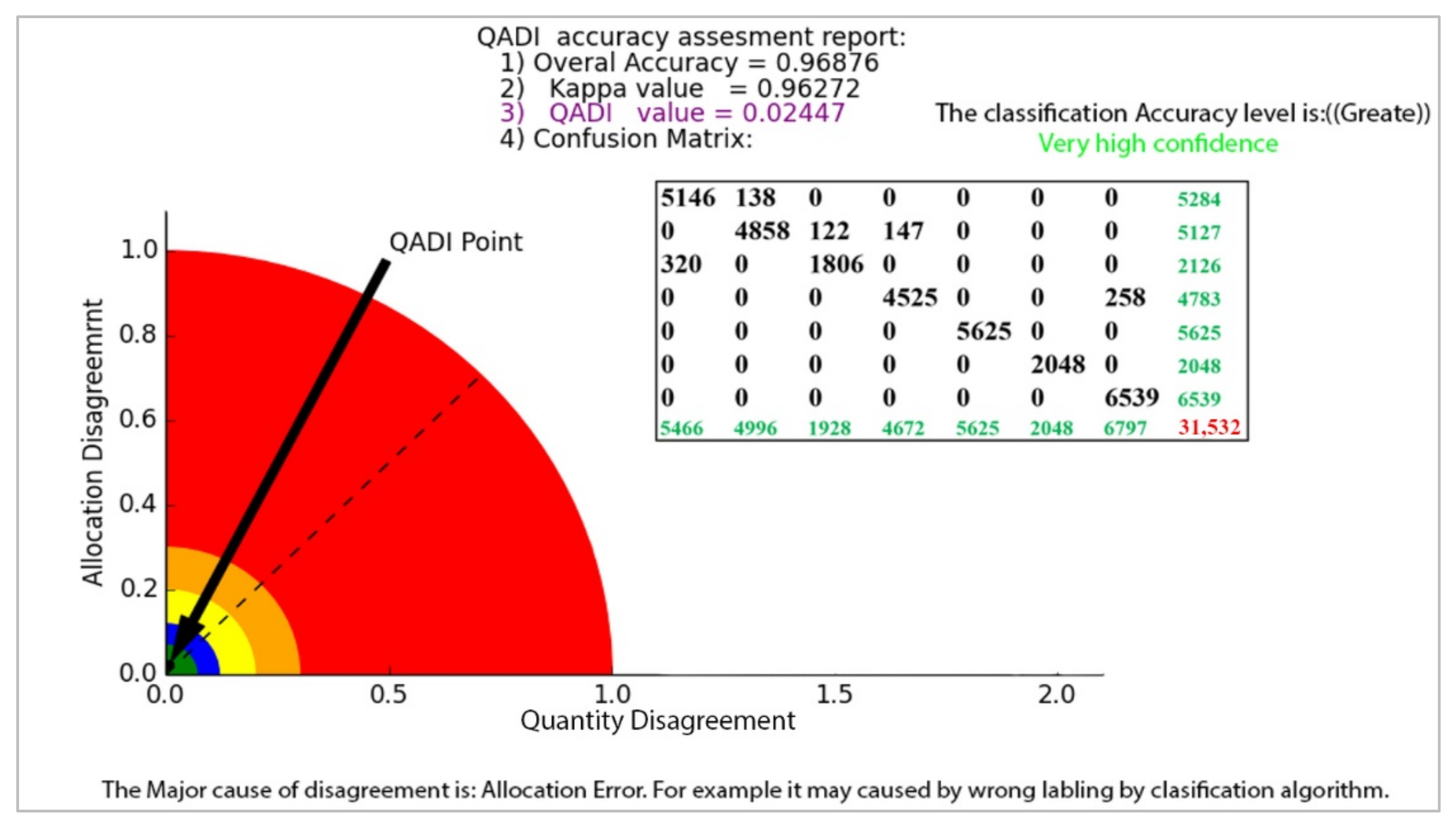
| User/Reference | Grass | Trees | Algae | Roads | Water Body | Bare Soil | Built up Area | Sum |
|---|---|---|---|---|---|---|---|---|
| Grass | 5146 | 138 | 0 | 0 | 0 | 0 | 0 | 5284 |
| Trees | 0 | 4858 | 122 | 147 | 0 | 0 | 0 | 5127 |
| Algae | 320 | 0 | 1806 | 0 | 0 | 0 | 0 | 2126 |
| Roads | 0 | 0 | 0 | 4525 | 0 | 0 | 258 | 4783 |
| Water body | 0 | 0 | 0 | 0 | 5625 | 0 | 0 | 5625 |
| Bare Soil | 0 | 0 | 0 | 0 | 0 | 2048 | 0 | 2048 |
| Built up area | 0 | 0 | 0 | 0 | 0 | 0 | 6539 | 6539 |
| Column total | 5466 | 4996 | 1928 | 4672 | 5625 | 2048 | 6797 | 31,532 |
| Overall accuracy | 0.97 | |||||||
| Kappa | 0.93 | |||||||
| User/Reference | W | RA | SL | FA | BL | OIA | Sum |
|---|---|---|---|---|---|---|---|
| Water(W) | 11 | 0 | 1 | 1 | 0 | 0 | 13 |
| Residential area (RA) | 0 | 48 | 0 | 0 | 2 | 1 | 51 |
| Salty lands (SL) | 1 | 0 | 39 | 2 | 0 | 0 | 42 |
| Farm agriculture (FA) | 0 | 2 | 0 | 72 | 1 | 1 | 76 |
| Bare lands (BL) | 1 | 0 | 2 | 0 | 65 | 1 | 69 |
| Orchard and irrigated agriculture (OIA) | 0 | 1 | 0 | 2 | 1 | 66 | 70 |
| Column total | 13 | 51 | 42 | 77 | 69 | 69 | 320 |
| Accuracy | 0.84 | 0.94 | 0.92 | 0.93 | 0.94 | 0.95 | |
| Overall Accuracy = 0.94 | |||||||
| Kappa = 0.92 | |||||||
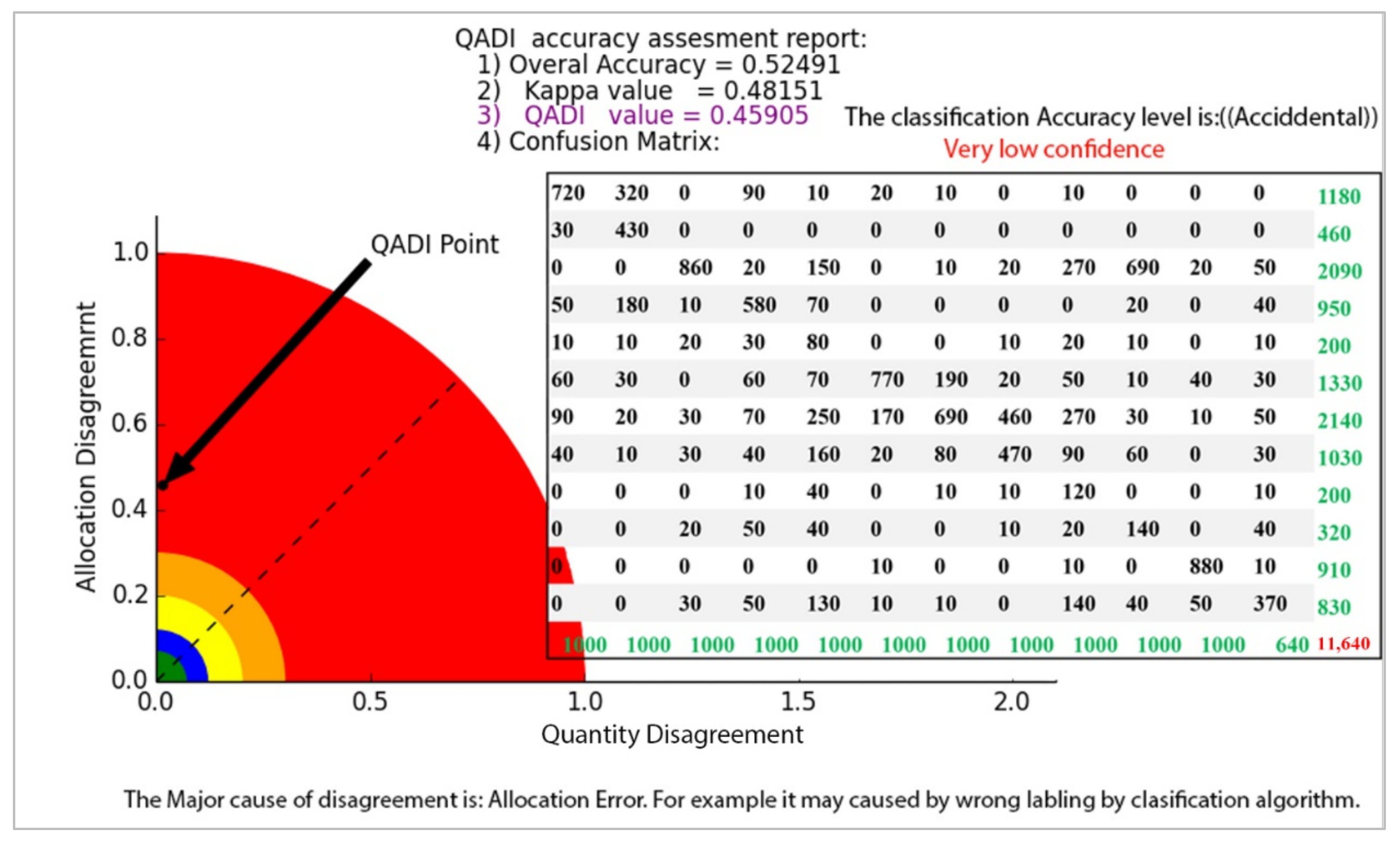
| a | b | c | d | e | f | g | h | i | j | k | l | |
|---|---|---|---|---|---|---|---|---|---|---|---|---|
| Urban areas (a) | 720 | 320 | 0 | 90 | 10 | 20 | 10 | 0 | 10 | 0 | 0 | 0 |
| Industrial Areas (b) | 30 | 430 | 0 | 0 | 0 | 0 | 0 | 0 | 0 | 0 | 0 | 0 |
| Worksites and mines (c) | 0 | 0 | 860 | 20 | 150 | 0 | 10 | 20 | 270 | 690 | 20 | 50 |
| Road Networks (d) | 50 | 180 | 10 | 580 | 70 | 0 | 0 | 0 | 0 | 20 | 0 | 40 |
| Trails (e) | 10 | 10 | 20 | 30 | 80 | 0 | 0 | 10 | 20 | 10 | 0 | 10 |
| Forests (f) | 60 | 30 | 0 | 60 | 70 | 770 | 190 | 20 | 50 | 10 | 40 | 30 |
| Medium-density Vegetation (g) | 90 | 20 | 30 | 70 | 250 | 170 | 690 | 460 | 270 | 30 | 10 | 50 |
| Low-density vegetation (h) | 40 | 10 | 30 | 40 | 160 | 20 | 80 | 470 | 90 | 60 | 0 | 30 |
| Bare rocks (i) | 0 | 0 | 0 | 10 | 40 | 0 | 10 | 10 | 120 | 0 | 0 | 10 |
| Bare soil (j) | 0 | 0 | 20 | 50 | 40 | 0 | 0 | 10 | 20 | 140 | 0 | 40 |
| Water surfaces (k) | 0 | 0 | 0 | 0 | 0 | 10 | 0 | 0 | 10 | 0 | 880 | 10 |
| Engravements (l) | 0 | 0 | 30 | 50 | 130 | 10 | 10 | 0 | 140 | 40 | 50 | 370 |
| Column total | ||||||||||||
| Overall accuracy | 0.52 | |||||||||||
| Kappa | 0.48 | |||||||||||
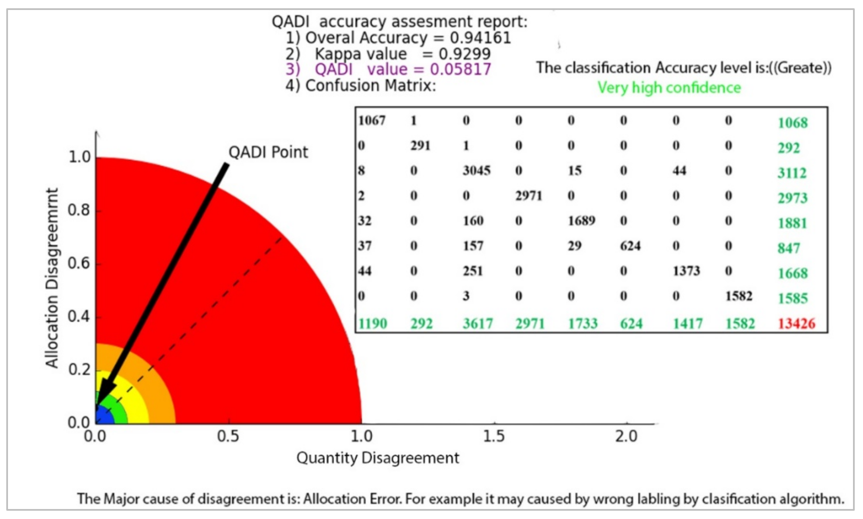
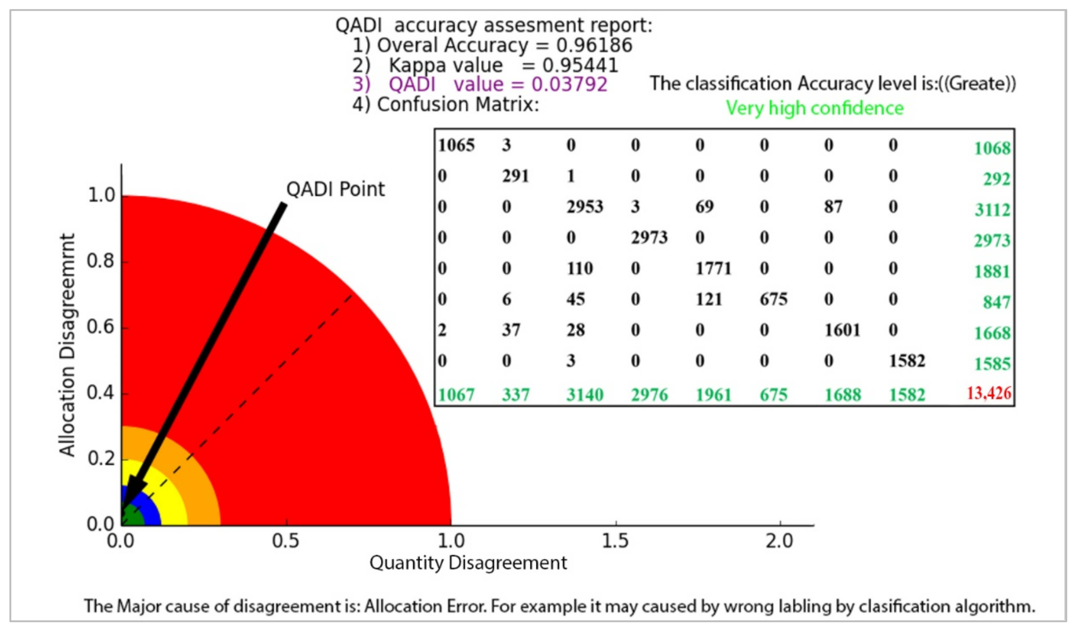
| LULC | Deep Water | Shallow Water | Urban | Bare Soil | Agricultural Land | Grassland | Forest | Cloud | Sum |
|---|---|---|---|---|---|---|---|---|---|
| Deep water | 1067 | 1 | 0 | 0 | 0 | 0 | 0 | 0 | 1068 |
| Shallow water | 0 | 291 | 1 | 0 | 0 | 0 | 0 | 0 | 292 |
| Urban | 8 | 0 | 3045 | 0 | 15 | 0 | 44 | 0 | 3112 |
| Bare soil | 2 | 0 | 0 | 2971 | 0 | 0 | 0 | 0 | 2973 |
| Agricultural land | 32 | 0 | 160 | 0 | 1689 | 0 | 0 | 0 | 1881 |
| Grassland | 37 | 0 | 157 | 0 | 29 | 624 | 0 | 0 | 847 |
| Forest | 44 | 0 | 251 | 0 | 0 | 0 | 1373 | 0 | 1668 |
| Cloud | 0 | 0 | 3 | 0 | 0 | 0 | 0 | 1582 | 1585 |
| Sum | 1190 | 292 | 3617 | 2971 | 1733 | 624 | 1417 | 1582 | 13,426 |
| Overall accuracy | 0.94 | ||||||||
| Kappa | 0.93 | ||||||||
| LULC | Deep Water | Shallow Water | Urban | Bare Soil | Agricultural Land | Grassland | Forest | Cloud | Sum |
|---|---|---|---|---|---|---|---|---|---|
| 1066 | 1 | 0 | 0 | 0 | 0 | 1 | 0 | 1068 | |
| Shallow water | 0 | 289 | 1 | 0 | 0 | 1 | 1 | 0 | 292 |
| Urban | 0 | 0 | 3000 | 0 | 29 | 0 | 83 | 0 | 3112 |
| Bare soil | 0 | 0 | 0 | 2973 | 0 | 0 | 0 | 0 | 2973 |
| Agricultural land | 0 | 0 | 130 | 0 | 1751 | 0 | 0 | 0 | 1881 |
| Grassland | 0 | 0 | 71 | 0 | 103 | 673 | 0 | 0 | 847 |
| Forest | 0 | 0 | 21 | 0 | 0 | 1 | 1646 | 0 | 1668 |
| Cloud | 0 | 0 | 16 | 0 | 0 | 0 | 0 | 1569 | 1585 |
| Sum | 1066 | 290 | 3239 | 2973 | 1883 | 675 | 1731 | 1569 | 13,426 |
| Overall accuracy | 0.97 | ||||||||
| Kappa | 0.96 | ||||||||
| LULC | Deep Water | Shallow Water | Urban | Bare Soil | Agricultural Land | Grassland | Forest | Cloud | Sum |
|---|---|---|---|---|---|---|---|---|---|
| Deep water | 1065 | 3 | 0 | 0 | 0 | 0 | 0 | 0 | 1068 |
| Shallow water | 0 | 291 | 1 | 0 | 0 | 0 | 0 | 0 | 292 |
| Urban | 0 | 0 | 2953 | 3 | 69 | 0 | 87 | 0 | 3112 |
| Bare soil | 0 | 0 | 0 | 2973 | 0 | 0 | 0 | 0 | 2973 |
| Agricultural land | 0 | 0 | 110 | 0 | 1771 | 0 | 0 | 0 | 1881 |
| Grassland | 0 | 6 | 45 | 0 | 121 | 675 | 0 | 0 | 847 |
| Forest | 2 | 37 | 28 | 0 | 0 | 0 | 1601 | 0 | 1668 |
| Cloud | 0 | 0 | 3 | 0 | 0 | 0 | 0 | 1582 | 1585 |
| Sum | 1067 | 337 | 3140 | 2976 | 1961 | 675 | 1688 | 1582 | 13,426 |
| Overall accuracy | 0.96 | ||||||||
| Kappa | 0.95 | ||||||||
| Confusion Matrix with a Balanced Distribution | Confusion Matrix with a Skewed Distribution | ||
|---|---|---|---|
| Kappa | 0.73 | Kappa | −0.00068 |
| QADI | 0.2 | QADI | 0.2 |
Publisher’s Note: MDPI stays neutral with regard to jurisdictional claims in published maps and institutional affiliations. |
© 2022 by the authors. Licensee MDPI, Basel, Switzerland. This article is an open access article distributed under the terms and conditions of the Creative Commons Attribution (CC BY) license (https://creativecommons.org/licenses/by/4.0/).
Share and Cite
Feizizadeh, B.; Darabi, S.; Blaschke, T.; Lakes, T. QADI as a New Method and Alternative to Kappa for Accuracy Assessment of Remote Sensing-Based Image Classification. Sensors 2022, 22, 4506. https://doi.org/10.3390/s22124506
Feizizadeh B, Darabi S, Blaschke T, Lakes T. QADI as a New Method and Alternative to Kappa for Accuracy Assessment of Remote Sensing-Based Image Classification. Sensors. 2022; 22(12):4506. https://doi.org/10.3390/s22124506
Chicago/Turabian StyleFeizizadeh, Bakhtiar, Sadrolah Darabi, Thomas Blaschke, and Tobia Lakes. 2022. "QADI as a New Method and Alternative to Kappa for Accuracy Assessment of Remote Sensing-Based Image Classification" Sensors 22, no. 12: 4506. https://doi.org/10.3390/s22124506
APA StyleFeizizadeh, B., Darabi, S., Blaschke, T., & Lakes, T. (2022). QADI as a New Method and Alternative to Kappa for Accuracy Assessment of Remote Sensing-Based Image Classification. Sensors, 22(12), 4506. https://doi.org/10.3390/s22124506