
Wheel Slip Control Applied to an Electric Tractor for Improving Tractive Efficiency and Reducing Energy Consumption

 ,
,
Abstract
:1. Introduction
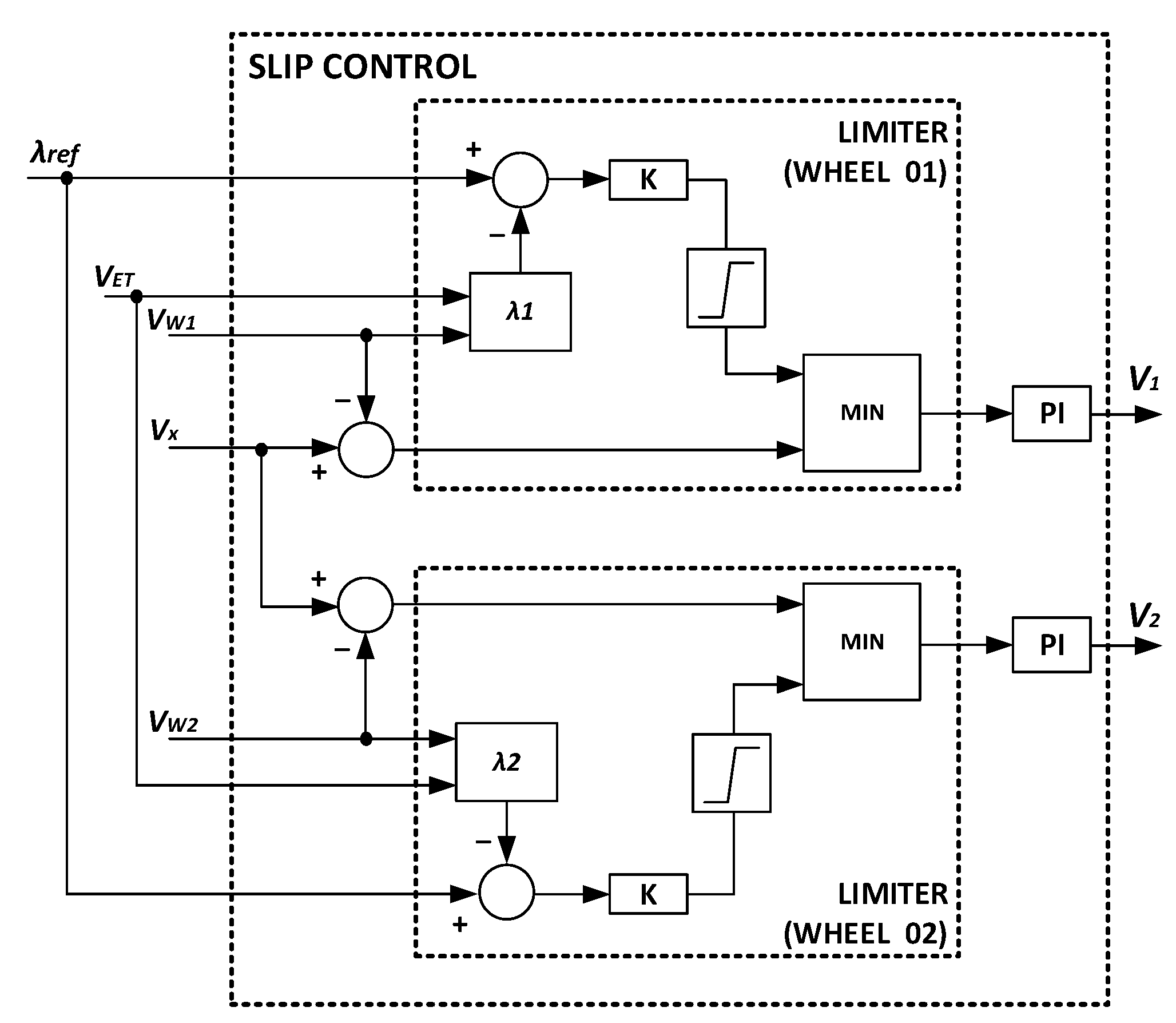
2. Proposed Control System
2.1. Tractor Model
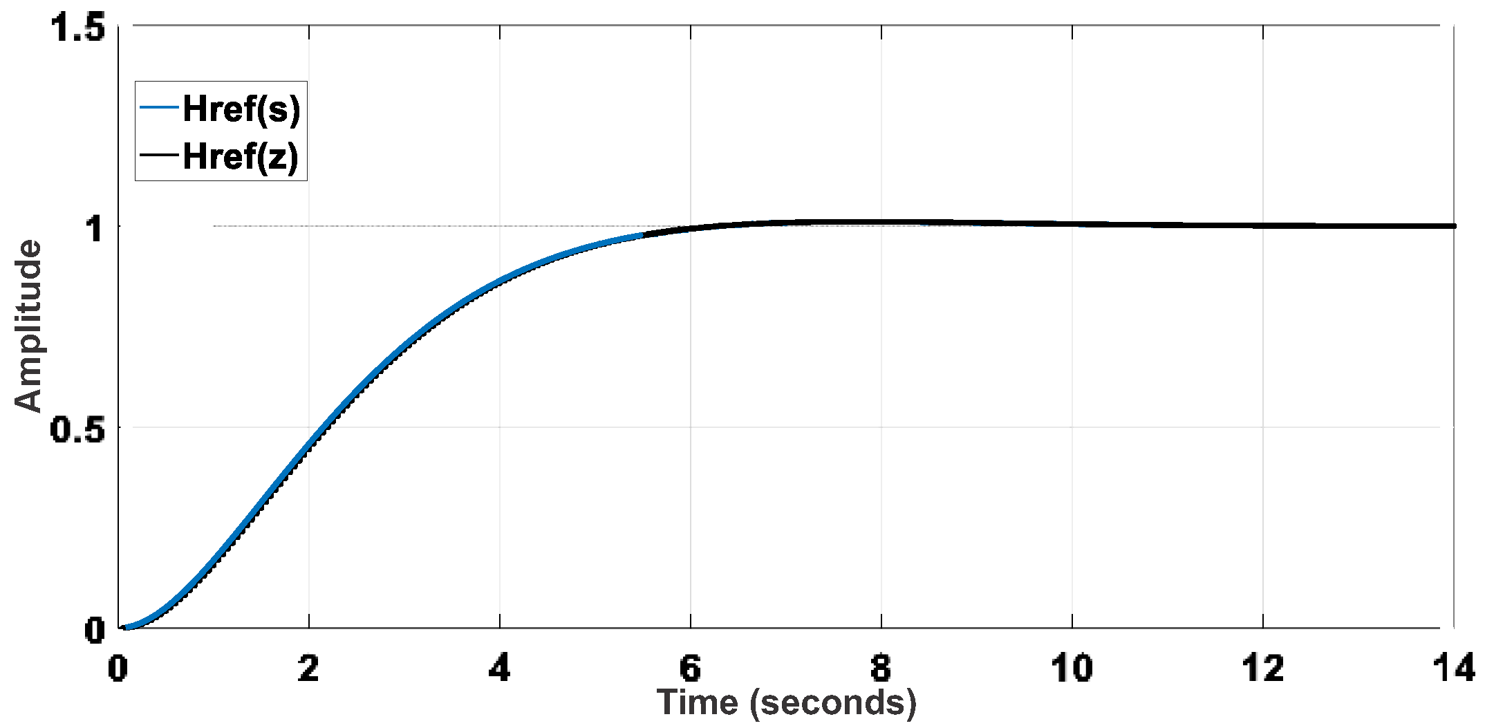
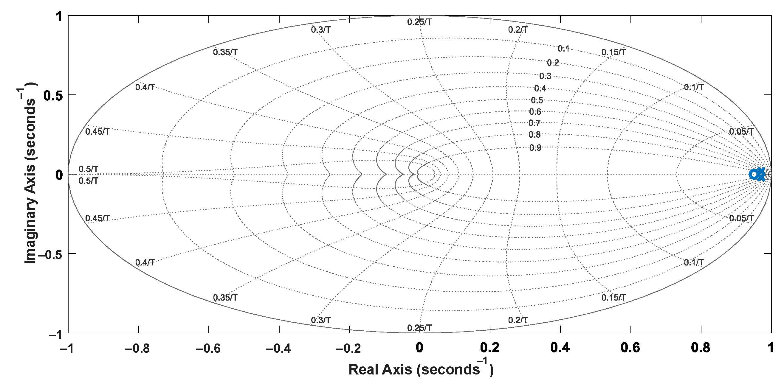
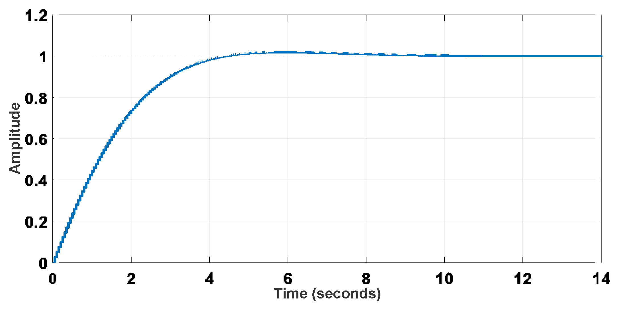
2.2. System Identification
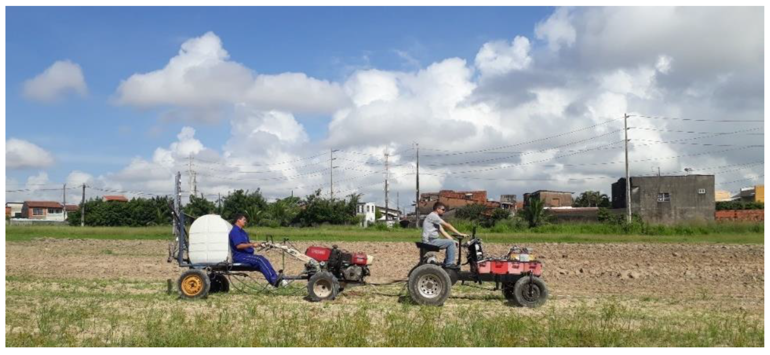
3. Experimental Results
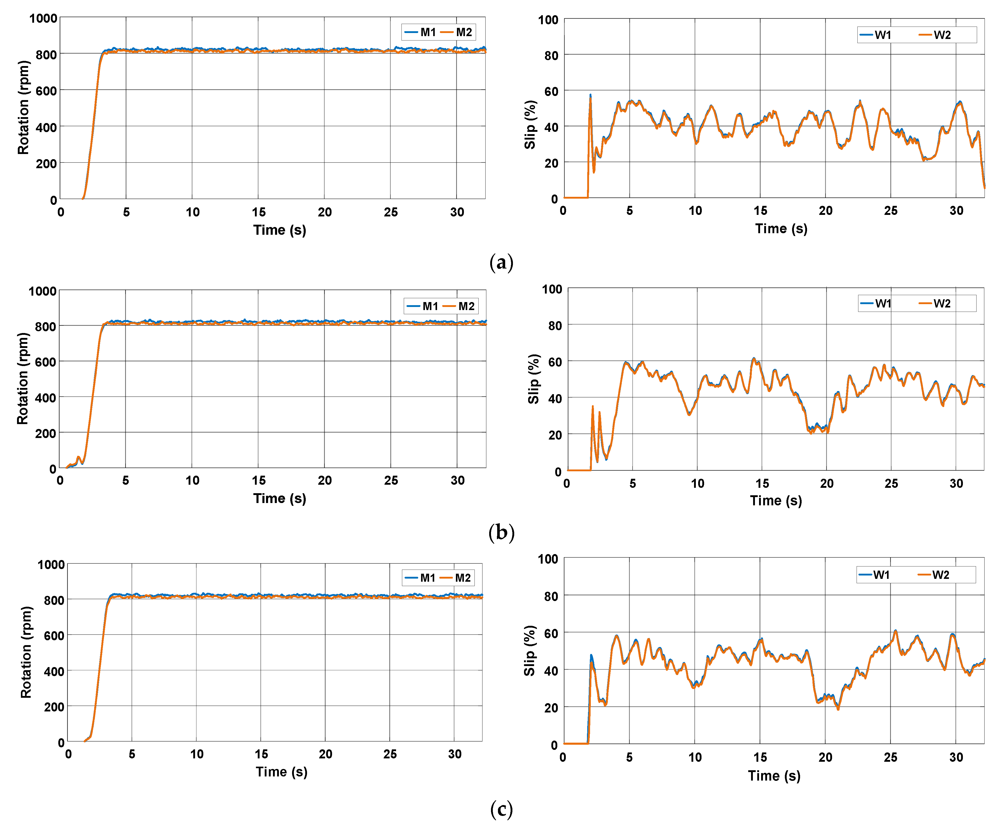
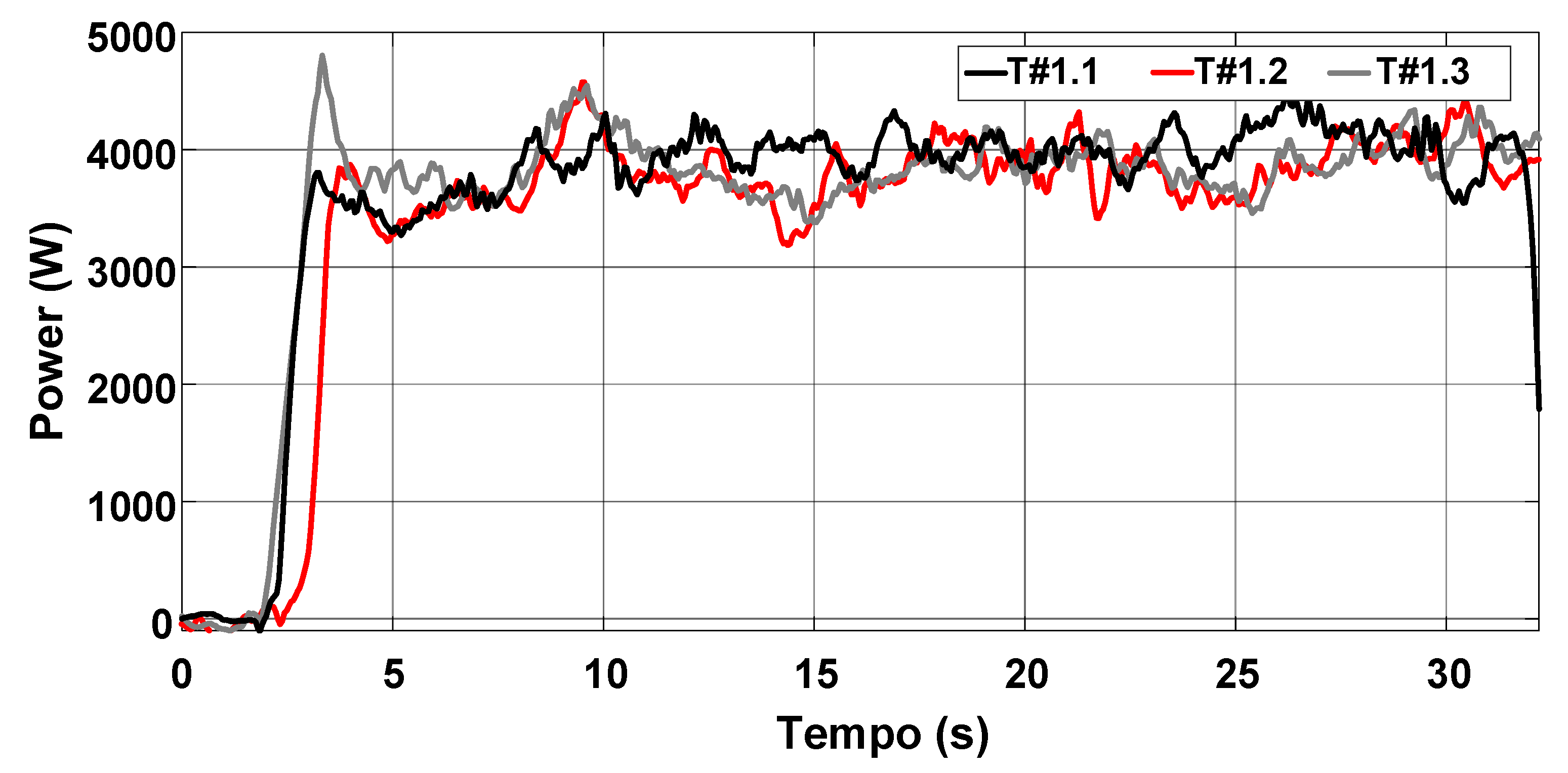
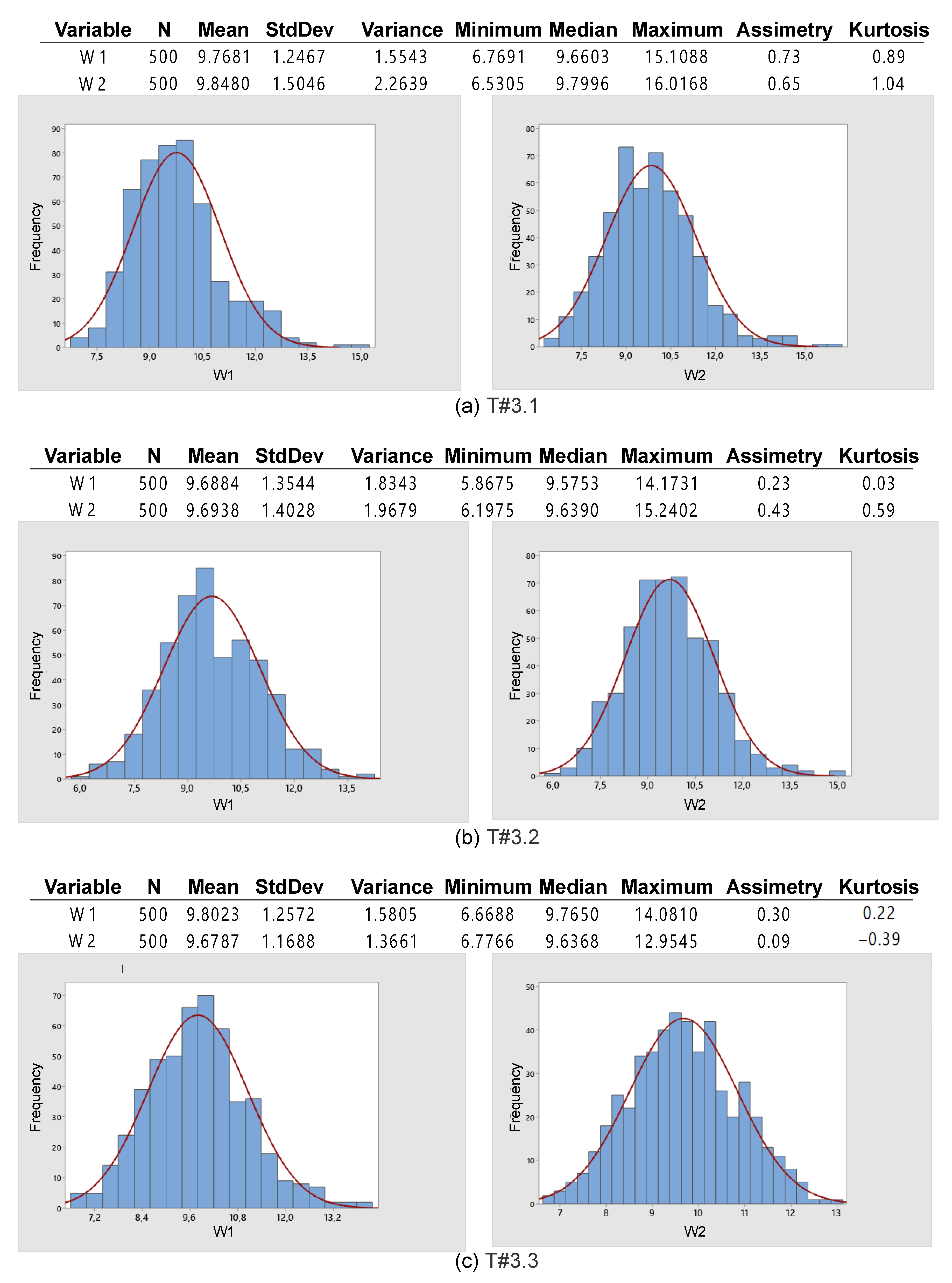
3.1. Test on Firm Soil without Slip Control
3.2. Test on Firm Soil with Slip Controlled by the Operator
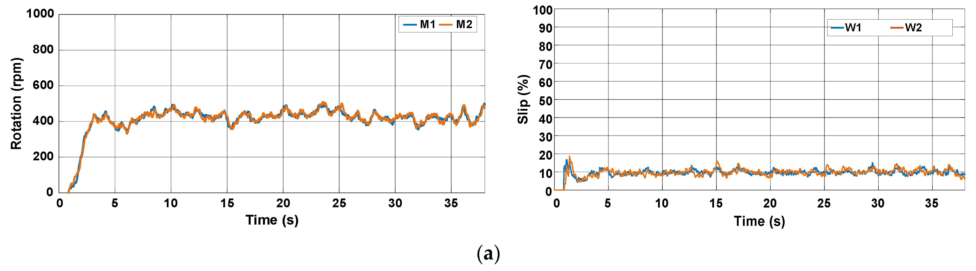
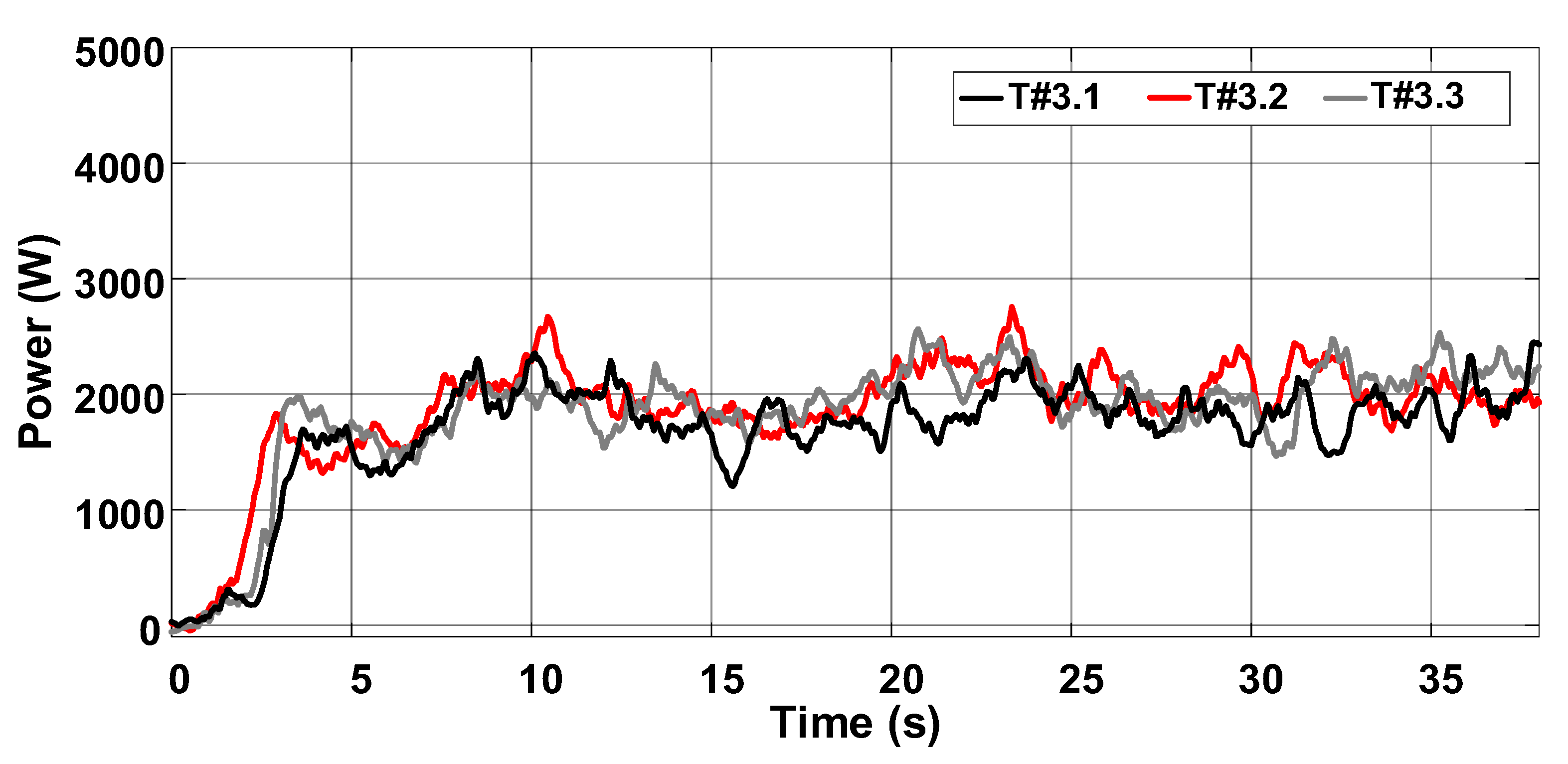
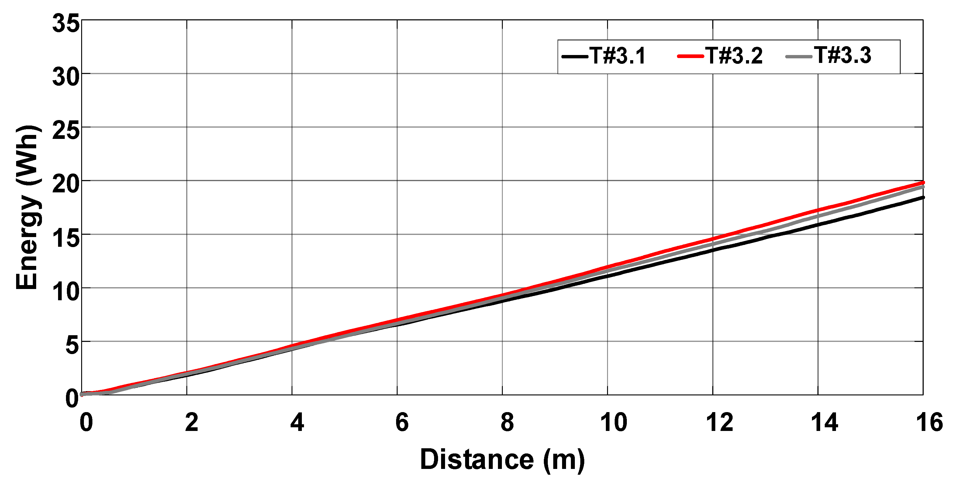
3.3. Test on Firm Soil with Slip Control
4. Conclusions
Author Contributions
Funding
Institutional Review Board Statement
Informed Consent Statement
Data Availability Statement
Conflicts of Interest
References
- Hensh, S.; Tewari, V.K.; Upadhyay, G. A novel wireless instrumentation system for measurement of PTO (power take-off) torque requirement during rotary tillage. Biosyst. Eng. 2021, 212, 241–251. [Google Scholar] [CrossRef]
- Osinenko, P.V.; Geissler, M.; Herlitzius, T. A method of optimal traction control for farm tractors with feedback of drive torque. Biosyst. Eng. 2015, 129, 20–33. [Google Scholar] [CrossRef]
- Gorjian, S.; Ebadi, H.; Trommsdorff, M.; Sharon, H.; Demant, M.; Schindele, S. The advent of modern solar-powered electric agricultural machinery: A solution for sustainable farm operations. J. Clean. Prod. 2021, 292, 126030. [Google Scholar] [CrossRef]
- Ghobadpour, A.; Mousazadeh, H.; Kelouwani, S.; Zioui, N.; Kandidayeni, M.; Boulon, L. An intelligent energy management strategy for an off-road plug-in hybrid electric tractor based on farm operation recognition. IET Electr. Syst. Transp. 2021, 11, 333–347. [Google Scholar] [CrossRef]
- Moreda, G.P.; Muñoz-García, M.A.; Barreiro, P. High voltage electrification of tractor and agricultural machinery—A review. Energy Convers. Manag. 2016, 115, 117–131. [Google Scholar] [CrossRef]
- Mocera, F.; Somà, A. Analysis of a parallel hybrid electric tractor for agricultural applications. Energies 2020, 13, 3055. [Google Scholar] [CrossRef]
- Mocera, F. A model-based design approach for a parallel hybrid electric tractor energy management strategy using hardware in the loop technique. Vehicles 2021, 3, 1–19. [Google Scholar] [CrossRef]
- Ueka, Y.; Yamashita, J.; Sato, K.; Doi, Y. Study on the development of the electric tractor: Specifications and traveling and tilling performance of a prototype electric tractor. Eng. Agric. Environ. Food 2013, 6, 160–164. [Google Scholar] [CrossRef]
- Chen, Y.; Xie, B.; Mao, E. Electric Tractor Motor Drive Control Based on FPGA. IFAC Pap. 2016, 49, 271–276. [Google Scholar] [CrossRef]
- Mousazadeh, H.; Keyhani, A.; Javadi, A.; Mobli, H.; Abrinia, K.; Sharifi, A. Life-cycle assessment of a solar assist plug-in hybrid electric tractor (SAPHT) in comparison with a conventional tractor. Energy Convers. Manag. 2011, 52, 1700–1710. [Google Scholar] [CrossRef]
- Wu, Z.; Xie, B.; Li, Z.; Chi, R.; Ren, Z.; Du, Y.; Inoue, E.; Mitsuoka, M.; Okayasu, T.; Hirai, Y. Modelling and verification of driving torque management for electric tractor: Dual-mode driving intention interpretation with torque demand restriction. Biosyst. Eng. 2019, 182, 65–83. [Google Scholar] [CrossRef]
- Liu, M.; Xu, L.; Zhou, Z. Design of a load torque based control strategy for improving electric tractor motor energy conversion efficiency. Math. Probl. Eng. 2016, 2016, 2548967. [Google Scholar] [CrossRef] [Green Version]
- Kim, W.-S.; Kim, Y.-J.; Park, S.-U.; Kim, Y.-S. Influence of soil moisture content on the traction performance of a 78-kW agricultural tractor during plow tillage. Soil Tillage Res. 2021, 207, 104851. [Google Scholar] [CrossRef]
- Ekinci, Ş.; Çarman, K. Effects of some properties of drive tires used in horticultural tractors on tractive performance. J. Agric. Sci. 2017, 23, 84–94. [Google Scholar]
- Shafaei, S.M.; Loghavi, M.; Kamgar, S. Fundamental realization of longitudinal slip efficiency of tractor wheels in a tillage practice. Soil Tillage Res. 2021, 205, 104765. [Google Scholar] [CrossRef]
- Osinenko, P.; Geißler, M.; Herlitzius, T.; Streif, S. Experimental results of slip control with a fuzzy-logic-assisted unscented Kalman filter for state estimation. In Proceedings of the 2016 IEEE International Conference on Fuzzy Systems (FUZZ-IEEE), Vancouver, DC, Canada, 24–29 July 2016; pp. 501–507. [Google Scholar]
- Xie, B.; Wang, S.; Wu, X.; Wen, C.; Zhang, S.; Zhao, X. Design and hardware-in-the-loop test of a coupled drive system for electric tractor. Biosyst. Eng. 2022, 216, 165–185. [Google Scholar] [CrossRef]
- Wen, C.-K.; Zhang, S.-L.; Xie, B.; Song, Z.-H.; Li, T.-H.; Jia, F.; Han, J.-G. Design and verification innovative approach of dual-motor power coupling drive systems for electric tractors. Energy 2022, 247, 123538. [Google Scholar] [CrossRef]
- Zhang, S.; Xie, B.; Wen, C.; Zhao, Y.; Du, Y.; Zhu, Z.; Song, Z.; Li, L. Intelligent ballast control system with active load-transfer for electric tractors. Biosyst. Eng. 2022, 215, 143–155. [Google Scholar] [CrossRef]
- Sun, C.; Sun, P.; Zhou, J.; Mao, J. Travel reduction control of distributed drive electric agricultural vehicles based on multi-information fusion. Agriculture 2022, 12, 70. [Google Scholar] [CrossRef]
- Heydrich, M.; Ricciardi, V.; Ivanov, V.; Mazzoni, M.; Rossi, A.; Buh, J.; Augsburg, K. Integrated braking control for electric vehicles with in-wheel propulsion and fully decoupled brake-by-wire system. Vehicles 2021, 3, 145–161. [Google Scholar] [CrossRef]
- Sunusi, I.I.; Zhou, J.; Sun, C.; Wang, Z.; Zhao, J.; Wu, Y. Development of online adaptive traction control for electric robotic tractors. Energies 2021, 14, 3394. [Google Scholar] [CrossRef]
- Soylu, S.; Çarman, K. Fuzzy logic based automatic slip control system for agricultural tractors. J. Terramechanics 2021, 95, 25–32. [Google Scholar] [CrossRef]
- Pranav, P.; Tewari, V.; Pandey, K.; Jha, K. Automatic wheel slip control system in field operations for 2WD tractors. Comput. Electron. Agric. 2012, 84, 1–6. [Google Scholar] [CrossRef]
- Gupta, C.; Tewari, V.K.; Ashok Kumar, A.; Shrivastava, P. Automatic tractor slip-draft embedded control system. Comput. Electron. Agric. 2019, 165, 104947. [Google Scholar] [CrossRef]
- Baek, S.-Y.; Baek, S.-M.; Jeon, H.-H.; Kim, W.-S.; Kim, Y.-S.; Sim, T.-Y.; Choi, K.-H.; Hong, S.-J.; Kim, H.; Kim, Y.-J. Traction performance evaluation of the electric all-wheel-drive tractor. Sensors 2022, 22, 785. [Google Scholar] [CrossRef]
- Wang, L.; Zhai, Z.; Zhu, Z.; Mao, E. Path tracking control of an autonomous tractor using improved stanley controller optimized with multiple-population genetic algorithm. Actuators 2022, 11, 22. [Google Scholar] [CrossRef]
- Landau, I.D.; Zito, G. Digital Control Systems: Design, Identification and Implementation; Springer: Berlin/Heidelberg, Germany, 2006; Volume 130. [Google Scholar]
- Zaccarian, L.; Teel, A.R. Modern anti-windup synthesis. In Modern Anti-Windup Synthesis; Princeton University Press: Princeton, NJ, USA, 2011. [Google Scholar]
- Melo, R.R.; Antunes, F.L.M.; Daher, S.; Vogt, H.H.; Albiero, D.; Tofoli, F.L. Conception of an electric propulsion system for a 9 kW electric tractor suitable for family farming. IET Electr. Power Appl. 2019, 13, 1993–2004. [Google Scholar] [CrossRef]
- Scheaffer, R.L.; Mulekar, M.S.; McClave, J.T. Probability and Statistics for Engineers; Cengage Learning: Boston, MA, USA, 2010. [Google Scholar]
- Bender, F.E.; Douglass, L.W.; Kramer, A. Statistical Methods for Food and Agriculture; CRC Press: Boca Raton, FL, USA, 2020. [Google Scholar]
- Montgomery, D.C.; Runger, G.C. Applied Statistics and Probability for Engineers; John Wiley & Sons: Hoboken, NJ, USA, 2010. [Google Scholar]


| Parameter | T#1.1 | T#1.2 | T#1.3 |
|---|---|---|---|
| Execution time (15 m) (s) | 27.27 | 30.61 | 29.41 |
| Velocity (m/s) | 0.55 | 0.49 | 0.51 |
| Velocity (km/h) | 1.98 | 1.76 | 1.94 |
| Mean slip (W1/W2) (%) | 39.92/39.94 | 46.16/45.58 | 44.84/44.17 |
| Average current drawn from batteries (A) | 83.43 | 79.28 | 81.36 |
| Average power drawn from batteries (W) | 3968.68 | 3790.68 | 3889.88 |
| Energy consumption (Wh) | 29.5 | 31.34 | 32 |
| Parameter | T#2.1 | T#2.2 | T#2.3 |
|---|---|---|---|
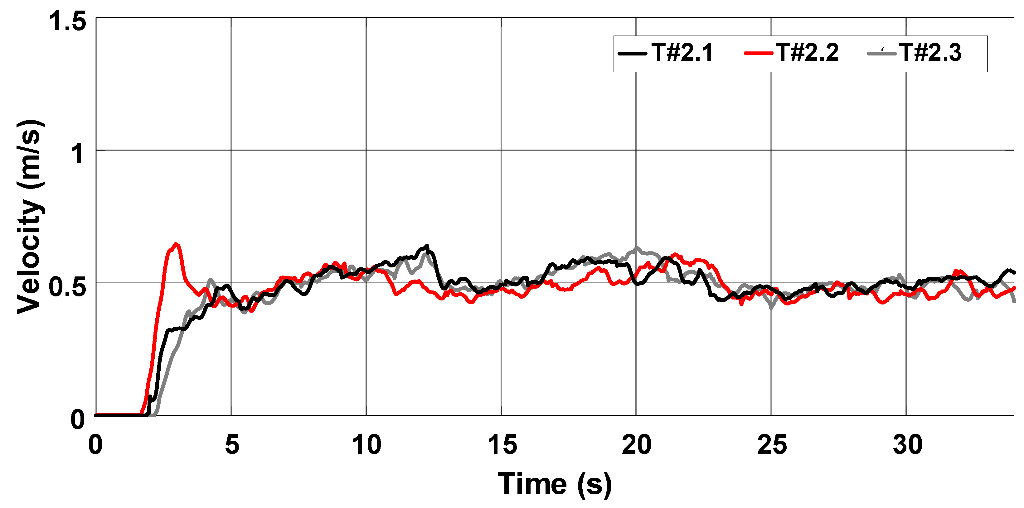
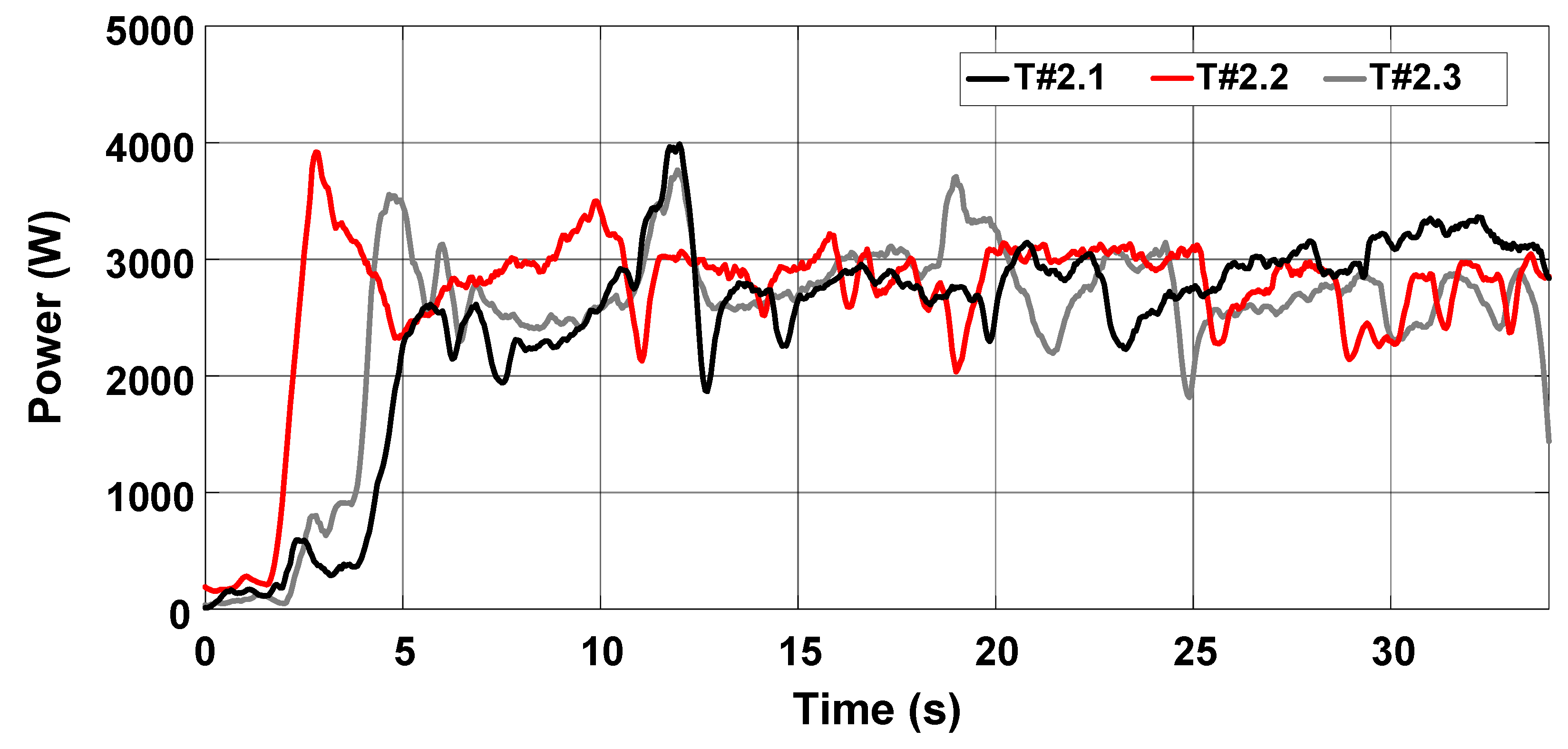
| Execution time (15 m) (s) | 29.41 | 30.61 | 28.85 |
| Velocity (m/s) | 0.51 | 0.49 | 0.52 |
| Velocity (km/h) | 1.83 | 1.76 | 1.87 |
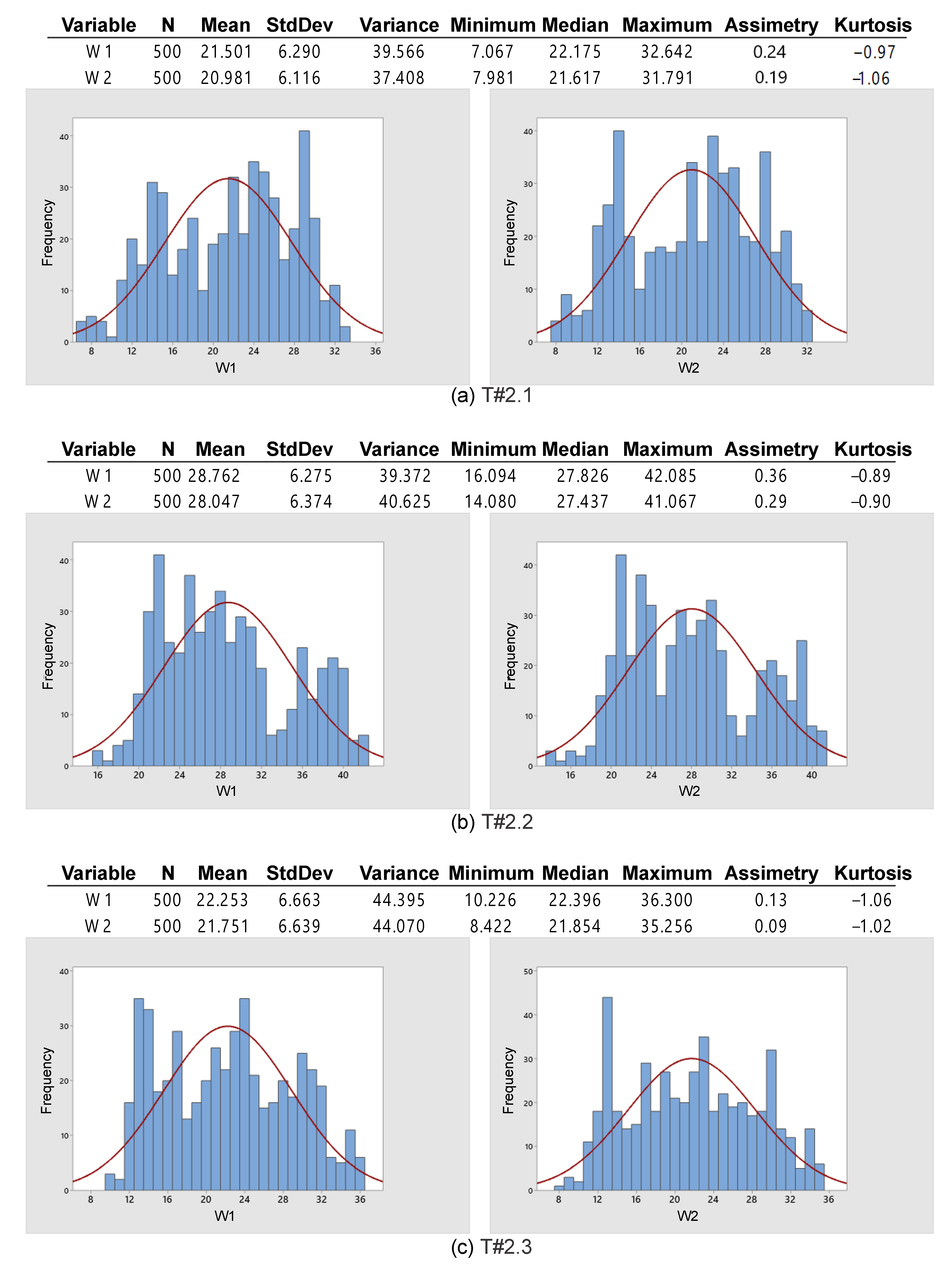
| Mean slip (W1/W2) (%) | 21.5/21.98 | 28.76/28.05 | 22.25/21.75 |
| Average current drawn from batteries (A) | 57.05 | 59.54 | 57.50 |
| Average power drawn from batteries (W) | 2742.94 | 2854.64 | 2766.99 |
| Energy consumption (Wh) | 21.94 | 24.51 | 22.5 |
| Parameter | T#3.1 | T#3.2 | T#3.3 |
|---|---|---|---|
| Execution time (15 m) (s) | 34.1 | 34.1 | 34.1 |
| Velocity (m/s) | 0.44 | 0.44 | 0.44 |
| Velocity (km/h) | 1.58 | 1.58 | 1.58 |
| Mean slip (W1/W2) (%) | 9.77/9.85 | 9.69/9.70 | 9.80/9.68 |
| Average current drawn from batteries (A) | 37.27 | 40.09 | 39.63 |
| Average power drawn from batteries (W) | 1820.18 | 1955.25 | 1931.35 |
| Energy consumption (Wh) | 17.1 | 18.55 | 18 |
Publisher’s Note: MDPI stays neutral with regard to jurisdictional claims in published maps and institutional affiliations. |
© 2022 by the authors. Licensee MDPI, Basel, Switzerland. This article is an open access article distributed under the terms and conditions of the Creative Commons Attribution (CC BY) license (https://creativecommons.org/licenses/by/4.0/).
Share and Cite
de Melo, R.R.; Tofoli, F.L.; Daher, S.; Antunes, F.L.M. Wheel Slip Control Applied to an Electric Tractor for Improving Tractive Efficiency and Reducing Energy Consumption. Sensors 2022, 22, 4527. https://doi.org/10.3390/s22124527
de Melo RR, Tofoli FL, Daher S, Antunes FLM. Wheel Slip Control Applied to an Electric Tractor for Improving Tractive Efficiency and Reducing Energy Consumption. Sensors. 2022; 22(12):4527. https://doi.org/10.3390/s22124527
Chicago/Turabian Stylede Melo, Rodnei Regis, Fernando Lessa Tofoli, Sérgio Daher, and Fernando Luiz Marcelo Antunes. 2022. "Wheel Slip Control Applied to an Electric Tractor for Improving Tractive Efficiency and Reducing Energy Consumption" Sensors 22, no. 12: 4527. https://doi.org/10.3390/s22124527