Abstract
This work focuses on improving a camera system for sensing a workspace in which dynamic obstacles need to be detected. The currently available state-of-the-art solution (MoveIt!) processes data in a centralized manner from cameras that have to be registered before the system starts. Our solution enables distributed data processing and dynamic change in the number of sensors at runtime. The distributed camera data processing is implemented using a dedicated control unit on which the filtering is performed by comparing the real and expected depth images. Measurements of the processing speed of all sensor data into a global voxel map were compared between the centralized system (MoveIt!) and the new distributed system as part of a performance benchmark. The distributed system is more flexible in terms of sensitivity to a number of cameras, better framerate stability and the possibility of changing the camera number on the go. The effects of voxel grid size and camera resolution were also compared during the benchmark, where the distributed system showed better results. Finally, the overhead of data transmission in the network was discussed where the distributed system is considerably more efficient. The decentralized system proves to be faster by 38.7% with one camera and 71.5% with four cameras.
1. Introduction
Increasing computing power allows more demanding tasks to be processed in less time. Despite this significant increase in computing power, the demands on the accuracy or volume of data processed are also increasing. Workspace monitoring is one example where such requirements grow even faster than computational power. There are multiple approaches to monitoring the environment. For example, depth measurement using time of flight [1,2,3] is not suitable for dynamic scenes. Structured light technology [4,5] is susceptible to ambient illumination. Passive sensing needs various textured objects. An extension for passive stereo vision offers an active approach [6], where a projector is added to a pair of cameras to project a pseudo-texture and enable better spatial sensing. Each has, of course, the positive aspects for which they were created and certain limitations. In general, several types of cameras or sensors can describe 3D environments and, nowadays, in great detail (millions of points) [7]. However, if a single sensor does not provide enough information, multi-camera systems can be used to combine information together [8]. It is necessary to think whether the whole environment needs to be captured in detail or focus should be given to a particular object. In any use of sensor systems, the primary focus is on the specific region of a workspace where the changes should be monitored in great detail. Thus, not all information obtained from sensors is relevant for subsequent use. It is almost always necessary to filter the input data to be satisfactory for the final product; for example, sensing people (namely for gaming using Kinect [9]), use in virtual reality, rehabilitation and similar situations from sensing people [10] to create 3D maps of the environment [11] requires specially designed filtering. It is possible to either filter static objects (the environment around people) or, on the contrary, filter known dynamic objects (e.g., a robotic arm). An important advantage is that it reduces the volume of data by removing information which is unnecessary for subsequent processing.
If we focus specifically on a workplace with a robot designed to collaborate with a human [12,13,14], it is required to monitor the workspace in which the robot can move without endangering the human.
Nowadays, many applications have been developed to improve Human–Robot Interaction (HRI) [15], which for example, use haptic feedback devices that notify a human worker about the currently planned trajectory and changes in the status of the robot [16,17]. An essential aspect of HRI is safety [18,19], in which robot avoidance against dynamic obstacles can be addressed using dynamically changing collision volumes [20,21], and alternatively, determining the robot’s speed based on detecting humans in the nearby space [22,23]. Nowadays, many applications are using neural networks [24,25] for detecting humans and predicting their movement [26,27].
For such a situation, it is necessary to filter a static workplace and a moving robot within it. There are already functional tools for such an application, such as MoveIt! [28], implemented in the ROS (Robotic Operating System)[29] environment. MoveIt! allows connection of 3D cameras and the use of post-processing to filter the workplace data so that only obstacle information is retained, e.g., in the form of voxels [30] as illustrated in Figure 1 by the green obstacle voxels.
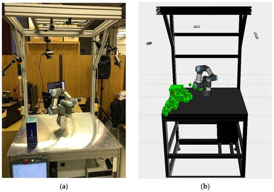
Figure 1.
Demonstration image of the output from MoveIt! filtration: (a) real workspace; (b) simulation.
For testing or research, MoveIt! is one of the possible solutions for a quick implementation. This framework has an adjustable perception module for monitoring changes in the workspace of a robot. This perception pipeline works by firstly defining the cameras’ configuration files and then connecting the corresponding communication topics with the data from the cameras.
However, for industrial applications, this module has its own limitations. For example, there is a limitation on the speed of updating camera data, which has a huge impact on usability in real industrial applications. There can be multiple devices in a ROS system that are connected in a local network, which provides sensor data. This allows connecting any number of cameras without overloading the USB ports on one computer. On the other hand, more demands are placed on the local network, as the sensor data is not transmitted via USB but via Ethernet or Wi-Fi. In addition, the cameras that are used by the system must be defined when the system is started, which represents a major limitation as this severely limits the flexibility of the system in terms of a simple plug-and-play solution.
These limitations are due to the centralization of data processing from all cameras on one device.
The main contribution of this paper is a developed system to distribute process to separate units in the ROS structure. The communication is optimized so that the network is not overloaded (for processed data). Therefore, any unnecessary demands on the speed and structure of the network are not needed.
We present an easily implementable solution that enables a quick connection of multiple cameras to a system at runtime. Therefore, this system can be used for prototyping and the rapid reconfiguration of the workplace without restarting the entire monitoring subsystem, which makes it more flexible in terms of its ability to quickly adapt to various workplace-monitoring situations compared to conventional approaches.
2. Materials and Methods
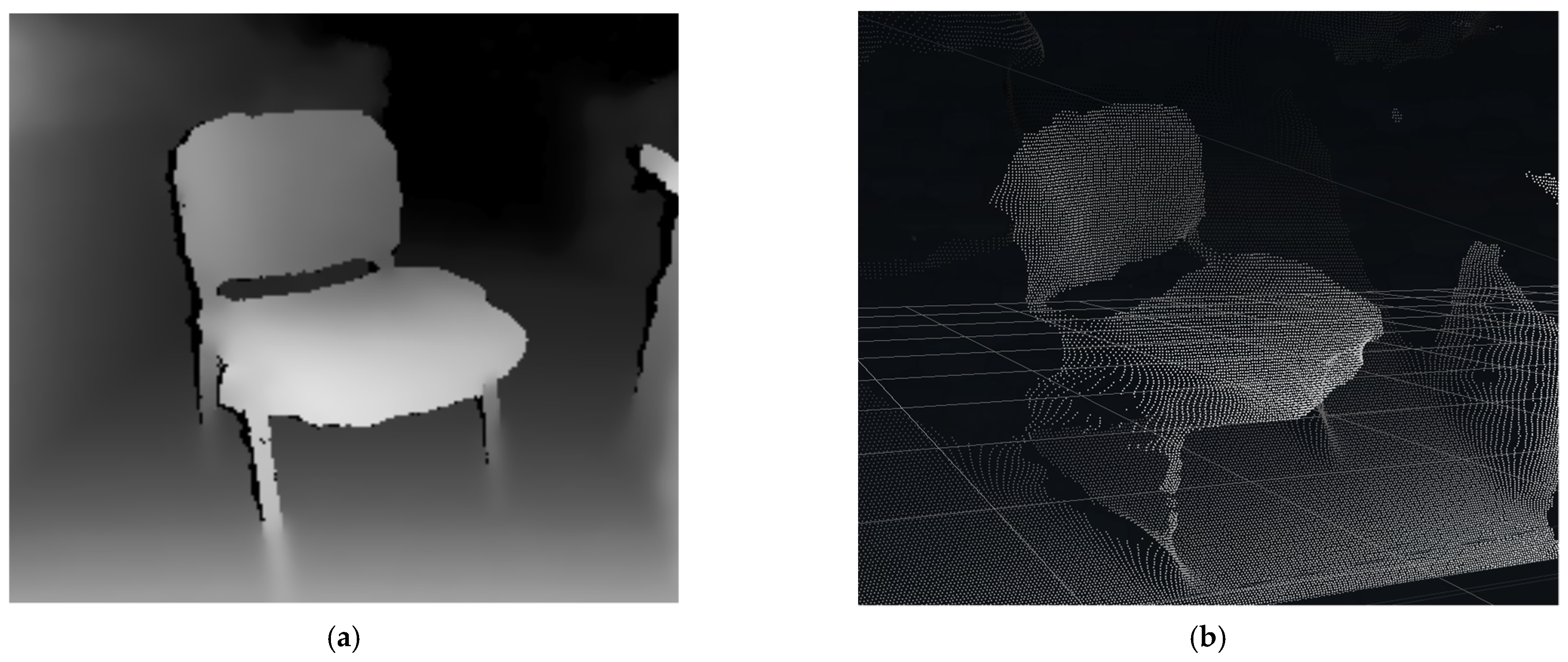
A fundamental aspect of 3D space representation is the form in which the environment is described. The most basic representation is the point cloud, which can be computed, for example, using stereo vision [7]. Based on the camera stream resolution, the number of points in space that correspond to each pixel in the depth image is obtained, see Figure 2.
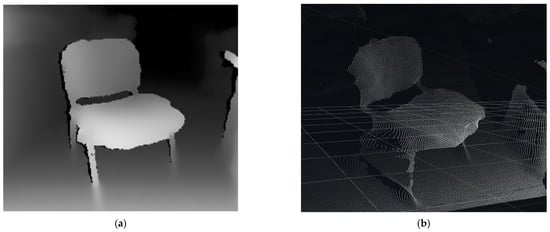
Figure 2.
3D chair data: (a) depth image; (b) point cloud.
Capturing the entire space with a single camera can be problematic, as the camera only captures the surfaces of obstacles in front of it. Another problem with using just a single camera is overshadowing an object with a different object in front of it. To create a more accurate representation of the obstacle using a depth image, it is necessary to utilize multiple cameras in the space to capture the obstacles at different angles. Such systems are known as multi-camera systems. As an example of the multi-camera system, our workstation with four cameras monitors the workplace with a UR3 robot, see Figure 3.
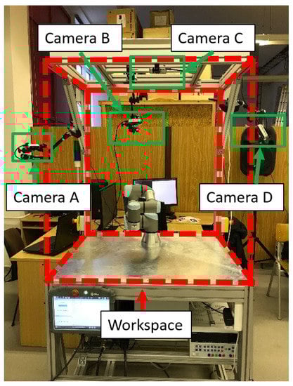
Figure 3.
Workspace with robot UR3.
With a multi-camera system, the workspace is scanned by multiple sensors, and the obtained data are then merged into a single representation. To fuse 3D data from multiple cameras, it is necessary to have a clearly defined camera position in space relative to a common base [31]. This can be achieved either by detecting visual markers [32] or by comparing point clouds relative to each other, from which the output is, for example, a transformation matrix. This matrix represents the rotation of the coordinate system around the x, y, and z axis and the displacement (1).
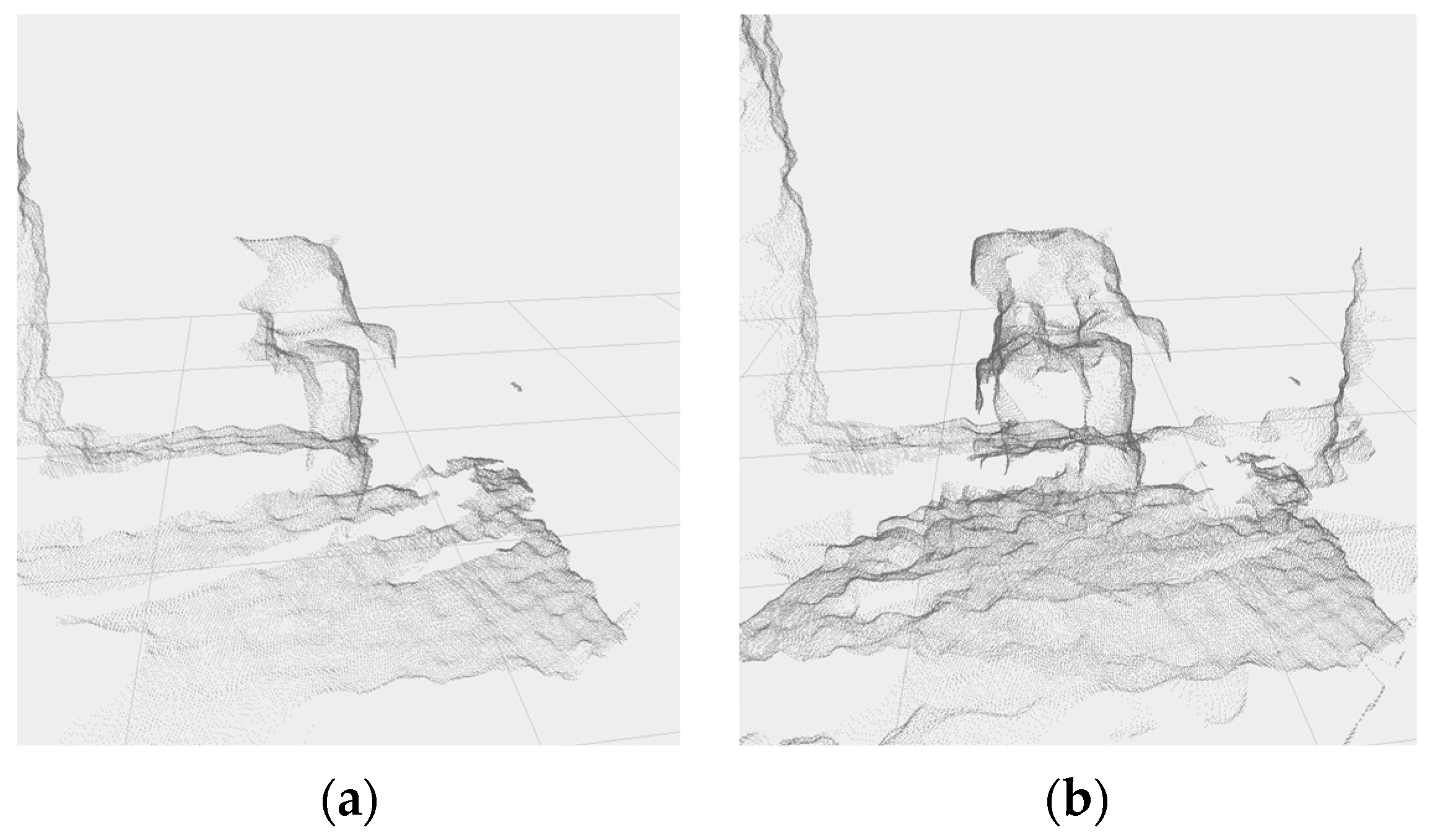
After the transformation, the individual point clouds are expressed relative to a single coordinate system and can be easily combined. The result is a single point cloud that describes the imaged workspace in more detail, Figure 4.
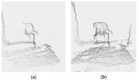
Figure 4.
Merged point clouds (data from camera Intel Realsense D435i with 1280 × 720 resolution) in the workplace coordinate system: (a) data from camera D; (b) data from cameras A and D (cameras transformation was calibrated by [32]).
This way of representing the space can achieve a detailed description of the environment, but usually, such a detailed model is not needed, and the computational power for processing a large number of points grows enormously. Therefore, the data are simplified to an acceptable resolution by voxelizing the point cloud. Voxelization can be performed in several ways [30,33,34,35]. In our case, this is carried out by aligning it to a voxel-sized grid, see Algorithm 1.
| Algorithm1 Voxelization |
| voxels = [] for point in pointCloud: voxel = Voxel() voxel.x = Floor(point.x/voxelSize + 0.5 * voxelSize) voxel.y = Floor(point.y/voxelSize + 0.5 * voxelSize) voxel.z = Floor(point.z/voxelSize + 0.5 * voxelSize) index = voxels.Exist(voxel) if(index ! = None): voxels[index].count += 1 else: voxels.Append(voxel) |
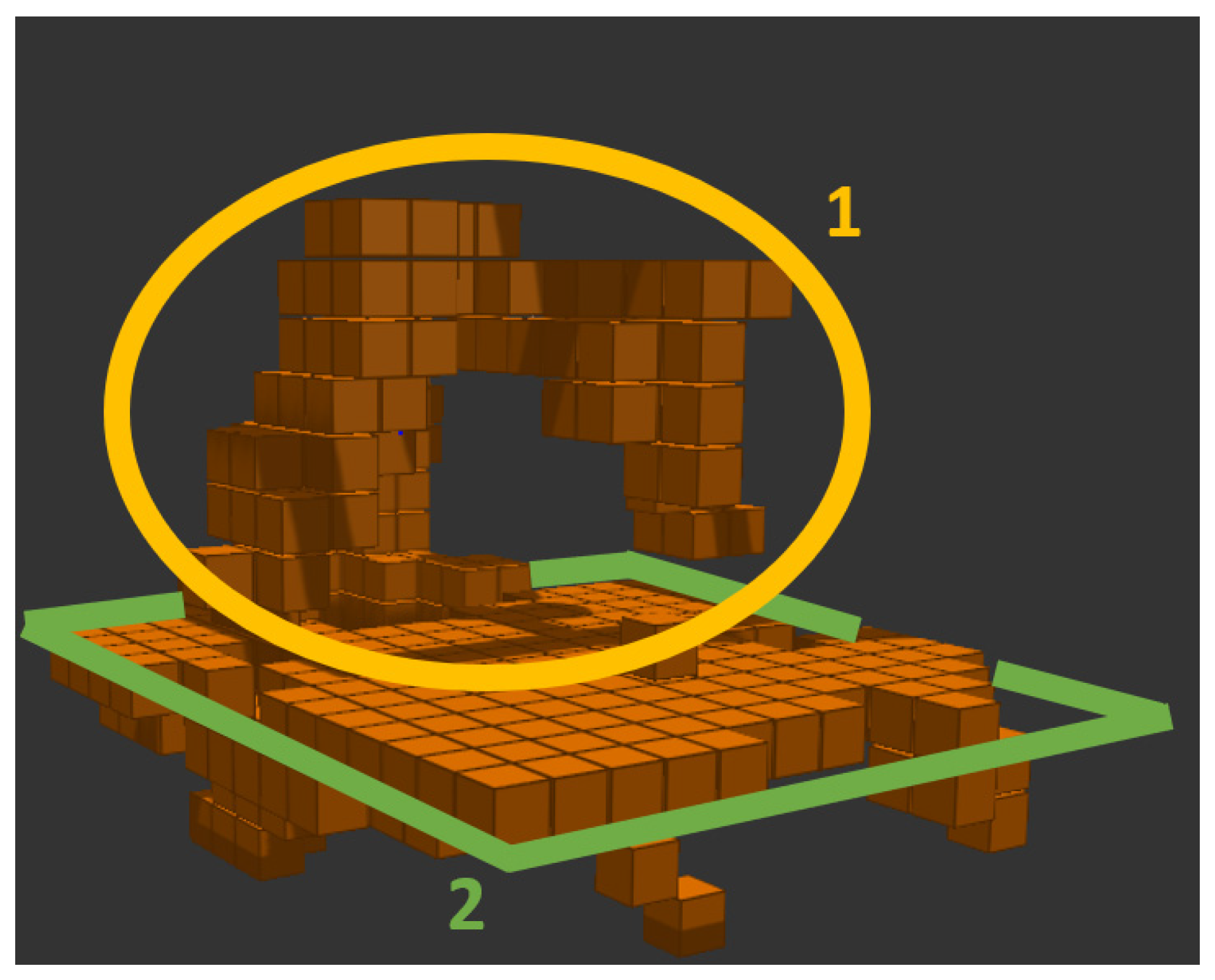
The result of voxelization is a voxel map expressed by a point cloud that represents the volume of a grid-sized cube. The voxel size (which ranges from 10 to 100 mm in 10 mm increments) is the same throughout the entire image at all locations and can be changed in real-time. If the robot workspace should be captured, having 3D information about the distant surroundings is unnecessary. Therefore, the voxel map can be cropped to the maximum dimensions of the workspace and thus reduce the resulting number of points in the map, see Figure 5.
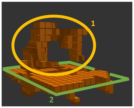
Figure 5.
Cropping voxel map to workspace: 1. robot; 2. robot workspace boundaries.
In this way, processed data are much more favorable for subsequent processing, although they still contain known objects. For example, the design of the workstation on which the robot is attached is clearly defined by the CAD model. This makes it unnecessary to capture this information and then reprocess it.
Therefore, filtering was implemented to filter the real data using an expected depth model. Expected depth can be obtained in two steps. First, the expected depth map is computed based on the perspective projection of 3D objects onto the 2D image, and then the expected depth for each pixel is computed, see Algorithm 2.
| Algorithm 2 Filter mask creation |
| depthImageExpected = [] models = database.GetActualScene() foreach mesh in models: transformationMatrix = mesh.PositionMatrix * camera.ViewMatrix * camera.ProjectionMatrix mesh.Transform(transformationMatrix) mesh.BackfaceCull() mesh.ViewportScale() depthImageExpected.Draw(mesh) |
If the workplace is described by CAD models (in our case, STL models that represent the model by triangles), the first step is to transform the model into its actual position relative to the camera. Then, using a perspective projection matrix (Equation (5), which is composed of Equations (1)–(4)), the model is projected to the camera view. Where FOV represents the field of view, aspectRatio is the ratio between the width and height of the camera stream, nearPlane is the closest plane the camera can detect, and farPlane is the farthest plane where the camera can reconstruct depth.
The values in the perspective matrix were derived from the real Intel Realsense D435i camera. This camera uses active stereo vision. To improve detection, it uses an infrared projector for depth sensing. Cameras sensing the workstation do not interfere with each other, as the infrared map just supports better triangulation.
To make the algorithm more efficient, all areas and faces of the 3D model that will be facing away from the camera view (hidden faces) were ignored. This is solved by checking the normals of the triangle area, see Algorithm 3.
| Algorithm 3 Backface culling |
| for triangle in mesh.Triangles: vectAB = triangle.vertex [1]–triangle.vertex [0] vectAC = triangle.vertex [2]–triangle.vertex [0] normal = Cross(vectAB, vectAC) if(normal.z > 0): triangle.visible = false |
Since the model vertices are mapped (by projection matrix) to a range of <−1, 1> in both the X and Y axes, Algorithm 4 describes a general procedure to map triangle vertices to an arbitrary camera stream resolution, which, in turn, is dependent on the current depth stream setting.
| Algorithm 4 Viewport scale |
| for triangle in mesh.Triangles: for vertex in triangle: vertex.x = int(vertex.x*wResolution/2) + wResolution/2 vertex.y = int(vertex.y*hResolution/2) + hResolution/2 |
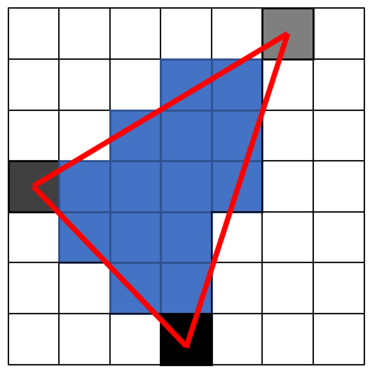
At this point, there are already specific pixels of triangle vertices with expected depth. The depth represented by the greyscale of each vertex of the triangle is then interpolated for pixels inside the triangle (blue), see Figure 6.

Figure 6.
Triangle depth rasterizing.
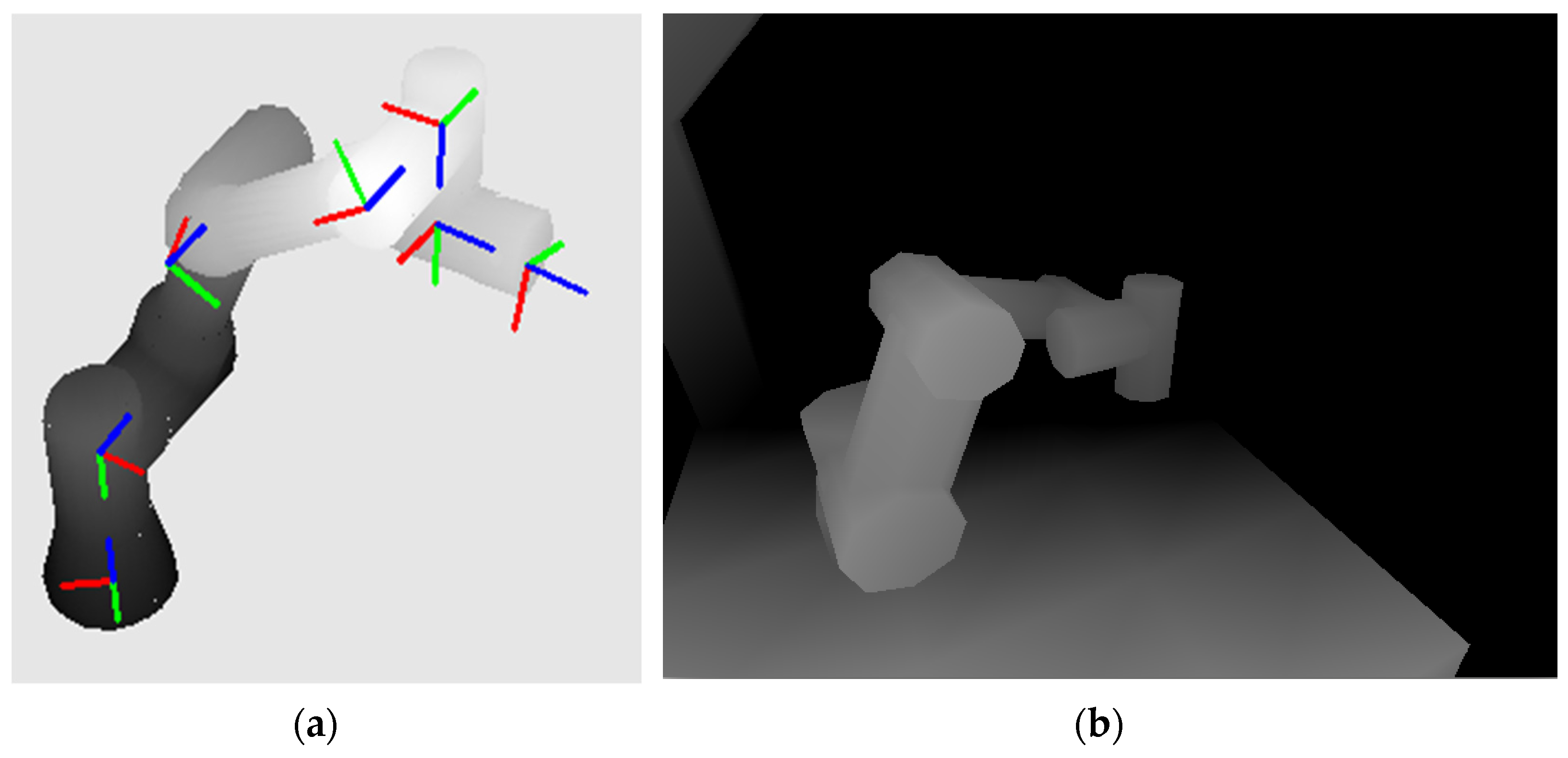
In this way, all the visible faces (triangles) of the objects wanted to project into the depth image are drawn. There are also objects on the workstation described by CAD models but dependent on the current configuration, such as a robot. These objects need to be reconstructed from the current joint variables. Standard robots are described using Denavit–Hartenberg (DH) parameters that represent the relationship between the coordinate systems based on the current joint rotation [36]. Therefore, the actual matrices of the individual robot link displacements at the workstation must be derived sequentially. The transformation matrix for each joint is shown in Algorithm 5.
where ϑi represents rotation around the Zi−1 axis (joint variable), d1 represents translation along the Zi−1 axis, ai represents translation along the Xi−1 axis, and αi represents rotation around the Xi axis, i.e., those kinematic parameters follow standard Denavit–Hartenberg convention.
| Algorithm 5 Transformation matrix of individual robot elements |
| for i in range(6): |
The result is a reconstructed robot model according to the actual joint rotations, see Figure 7a. In Figure 7b, the result of an expected depth image created from the CAD models of the workspace and the actual position of the UR3 robot is shown.
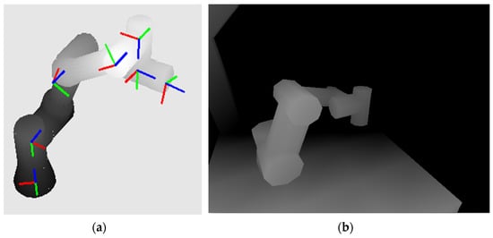
Figure 7.
Rendered UR3 robot: (a) with coordinate systems attached to individual links according to the Denavit–Hartenberg principle (the blue z-axes represent the axes of rotation); (b) reconstructed expected depth map of the workspace.
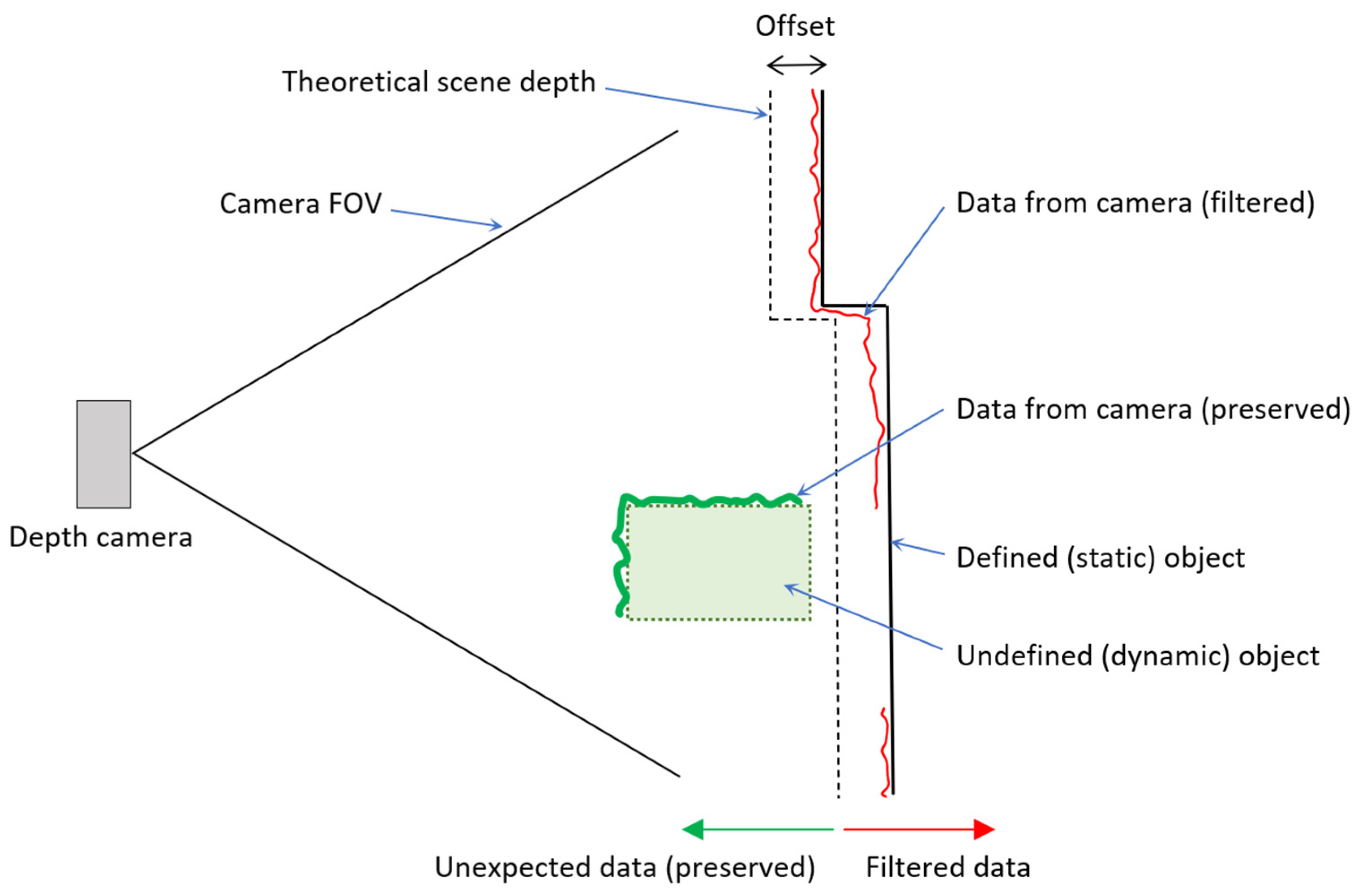
Once the actual scene has been completely reconstructed (Defined static/dynamic object), the real workspace scene obtained by the cameras can be compared with the calculated expected depth image. However, it is necessary to realize that the real camera captures with certain accuracy (data from the camera), and it is impossible to compare the real and expected depth exactly. Therefore, a sufficient offset needs to be added to cover the inaccuracy of the camera sensing, see Figure 8. This approach filters out all objects where the distance of expected depth (with offset) is less than the distance of the actual depth. The diagram shows the principle where the environment is defined (as a line Defined (static) object). The expected depth of the scene is identical to the real one but is offset to capture the basic inaccuracy of the camera (data from the camera(filtered)—red line). The un-defined (dynamic) object is before the expected depth (from the camera view), so this data is not filtered.
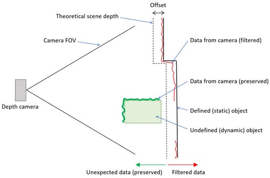
Figure 8.
Illustration of filtration principle.
It is impossible to filter out all image noise by comparing the real and expected depth images. Therefore, was implemented a post-processing filter which determines whether a voxel is a noise voxel or an actual object surface based on the density of points in the voxel.
The maximum possible density of points representing a voxel is variable based on the distance from the camera. The relationship between voxel occupancy and distance for a 5 cm voxel and the resolution of the Intel RealSense D435i 640 × 480 [px] camera is shown in Figure 9. It depicts the count of points per voxel according to the minimum and maximum possible sensing distance of the camera.
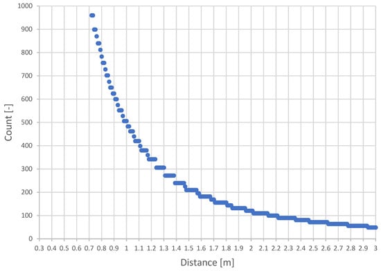
Figure 9.
Density of expected points of a voxel depending on the distance from the camera.
A simplified calculation of the maximum voxel capacity is described in Algorithm 6. First, the alpha angle is calculated, representing the maximum angle at which the rays of points can be projected. The density is then computed as the maximum number of rays that can fit into the alpha angle for pixels on the X and Y axis.
| Algorithm 6 Maximum number of points in a voxel |
| alfa = atan(voxelSize/voxel.distance) countPerRow = alfa/(hFOV/hResolution) countPerColumn = alfa/(wFOV/wResolution) countPerVoxel = countPerRow * countPerColumn |
The final filtering is then carried out by checking whether the actual voxel coverage is less than the density coverage with a certain threshold, and thus, these voxels are considered to be under-covered. Several factors affect the noise filtering threshold, e.g., ambient effects (sunlight) or camera lens calibration. In our case, this limit was around 50–60% of the maximum value to ensure that the filtering provides a satisfactory result. Hence, these voxels are removed as they represent noise, see Algorithm 7.
| Algorithm 7 Voxel filtering by occupancy percentage |
| for voxel in voxels: maxCount = GetExpectedCount(voxel.Size, voxel.Distance, camera.Info) if(voxel.count < maxCount * threshold) voxels.Delete(voxel) |
The output of these algorithms are only voxels representing objects that have not been defined at the workplace and thus are needed for subsequent processing, e.g., robot trajectory re-planning.
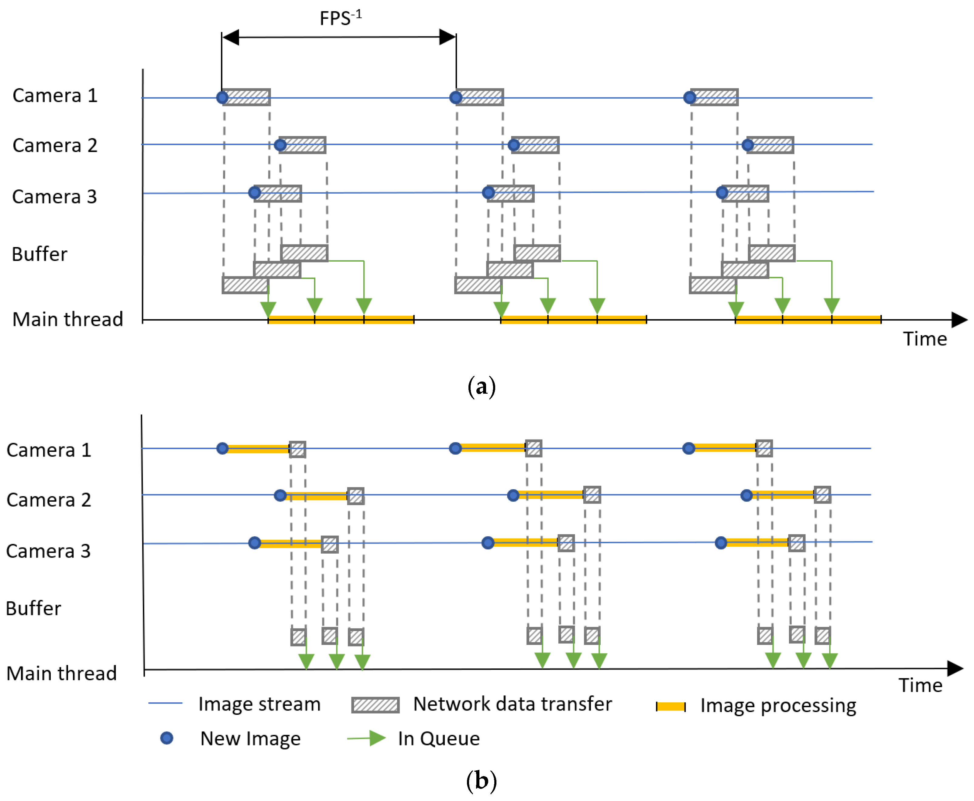
The entire filtering process is distributed to individual computing devices that process depth streams from just one camera, as shown in Figure 10. Each of these units filters the scene for a specific camera position on the site. For our system, Nvidia Jetson Nano and Intel RealSense D435i cameras were used.
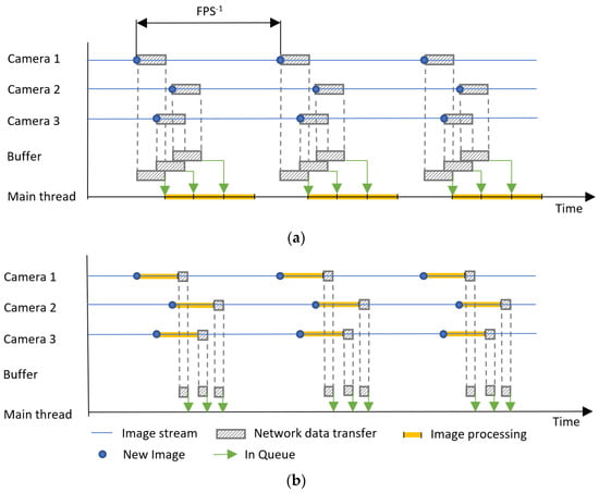
Figure 10.
Diagram of the system principle: (a) centralized; (b) distributed.
Figure 10 represents only symbolic block sizes and demonstrates the principle of a centralized and distributed system and the ratios do not correspond in any way to the real scenario. Figure 10 describes the case with three cameras at a general FPS (Frame Per Second).
In the initial setup of the cameras, all relative positions of the cameras to the robot coordinate system were obtained using a calibration grid board [27]. The system uses a single unit as the main camera, creating a server for initialization and a subsequent location for the descendant data, see Algorithm 8.
| Algorithm 8 Methods for Initialize and Update computing devices |
| def Initialize(device): if(initializedDevices.Exist(device.IP): return initializedDevice[device.IP].ID id = initializeDevices.Insert(device.IP) return id def Update(device): initializedDevices[device.ID].voxels = device.voxels return actualSceneValues |
The processed data from the individual units are combined in the main unit. Each computed datum is stored with a timestamp of when it was received to check for old data, see Algorithm 9. The verification is performed by comparing the time since the update of the data from the individual cameras. In other words, if the difference between the time of the arrival of data TU and actual time TA is less than Threshold (Equation (6)), the IsTimeStampValid condition is satisfied.
The units are not synchronized in the sense of camera frame acquisition. Each unit maintains its own framerate, and the most recent frame is sent to the master device, where it is used until a newer frame arrives (or the timestamp check fails).
Latency of the data update callback was measured as the time required for data transfer to the main device and transfer of the response data. The average transfer latency for 0 to 1000 voxels is 12 ms for each device (measured for four connected devices).
| Algorithm 9 Merging data from computing devices |
| globalVoxelMap = [] for device in initializedDevices: if(device.IsTimeStampValid())): globalVoxelMap.Insert(device.voxels) |
The Initialize method on the server represents the entry point for the processing units. When an initialization command arrives here, the incoming IP address is checked to see if it is already registered (behind one IP is expected one camera only). If it is registered, it represents a computing device that has been initialized in the past, and it is assumed that the device has been restarted either intentionally or due to a failure. No new memory space is created for such a computing device, and only its assigned ID is retrieved. The current workstation settings (e.g., robot position, filter parameters) are added to the ID. If the device IP is initialized for the first time, memory space is created that represents only the data from that unit. Allocated memory is represented by a dynamic list, and its initial size is for 150 voxels to avoid frequent increases in allocated memory. The output method then comprises the memory ID and following values, which represent the current settings (voxel size, robot configuration, percentage voxel occupancy, etc.), as is the case in pre-initialized devices.
The Update method is triggered if any computing unit updates the current data. The computing device that sends the data update also sends its ID. The server then deletes all previous data from that unit and replaces it with the new data. In addition, the timestamp of the newly arrived values is recorded so that the data can be checked to confirm whether the data is outdated for future data fusion.
When connected to the network, each computing device must initialize itself to obtain an ID under which it will then send the current local data it is currently capturing with the connected camera. A localization algorithm (in our case, 3D grid board detection) is used to find the position of the camera connected to a particular device. The depth map is then filtered using the 3D reconstruction of the site and the depth map comparison described above.
Using this structure, any number of computation devices with a camera (Jetson Nano; Nvidia, Santa Clara, CA, USA and D435i camera; Intel, Santa Clara, CA, USA) can be connected. Furthermore, the module is set up to run the filtering algorithms when the system starts automatically, so there is no need to have a device (e.g., keyboard, mouse, monitor, etc.) connected to each unit, and it will automatically start streaming the current data when the power is turned on.
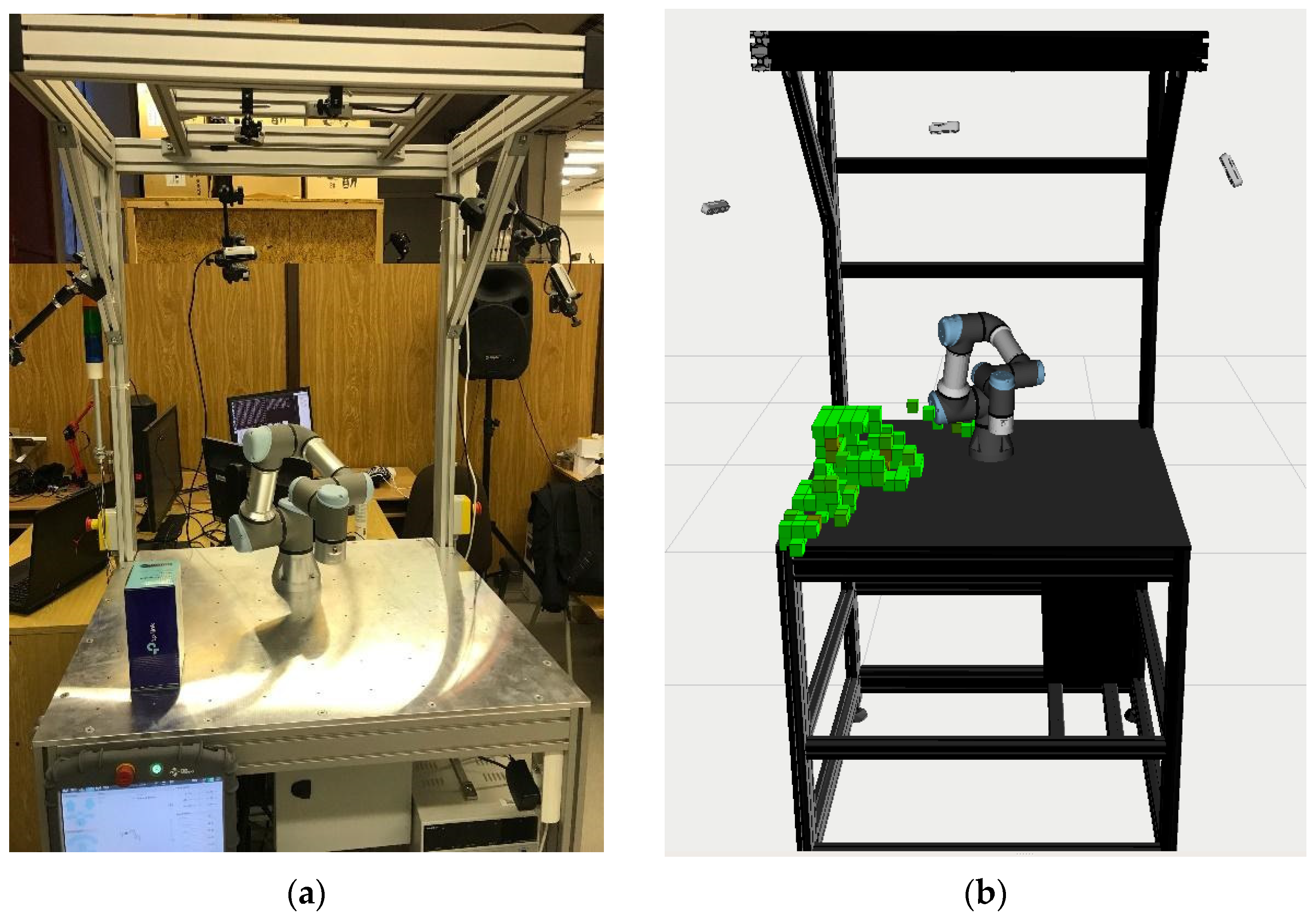
Based on the idea of distributing the computational power, algorithms have been proposed to filter the depth information in the dynamic environment (Figure 11a). This information was then thoroughly filtered (Figure 11c–e) so that the output data from the sensor system contained only the necessary information about unknown objects in the scene, see Figure 11b.
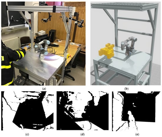
Figure 11.
Filtered scene by the distributed method: (a) real scenario; (b) 3D visualization; (c–e) camera bitmask.
3. Results and Discussion
The depth image processing speed and refresh rate of the entire workplace scene were compared using the distributed method versus the centralized (MoveIt!) method in a real workplace. It should be noted that the depth image filtering was performed differently by each method. In the distributed method, the computation was performed on the Jetson Nano unit processor (Quad-core ARM A57, 1.43 GHz, Memory 4 GB LPDDR4) [37], while in the centralized method, everything was computed on the laptop GPU (NVIDIA GeForce GTX 1070, 1.51 GB, CUDA Cores 1920, Memory 5 GB GDDR5) [38].
Variables such as the resolution of cameras, the size of the voxel map, and the number of cameras were used to compare the solutions. These factors affect the total performance of the solution with a major impact on the scene refresh rate, hence the need for measurements.
The scene refresh rate of the workstation was measured for the following depth stream resolutions with a setting of 15 FPS:
- 424 × 240;
- 640 × 480;
- 1280 × 720.
For all of these resolutions, the voxel grid size dependencies were measured, where the voxel size was measured from 10 to 100 mm in 10 mm increments. The actual measurement consisted of determining the time to compute the depth image from the time of its arrival to the filtering and the time to reconstruct the entire workstation scene from the reception of the data from the first camera to the evaluation of the filtering from the last camera. Table 1 and Table 2 compare the time for reconstructing the whole scene with three cameras, using both the centralized and distributed approaches. During the measurements, it was found that the centralized approach at higher resolutions was not able to provide a depth stream of 15 fps. At a resolution of 424 × 240, the framerate was maintained. At 640 × 480 resolution, the depth stream reached a maximum of 6 fps, and at 1280 × 720, it reached 2 fps. A low bandwidth of the depth stream then influences the processing time of the image. Furthermore, it was found that when the voxel size was less than 0.02 m, the depth filtering time increased rapidly: for 424 × 240 resolution, the time increased to 1.9 s; for 640 × 480 resolution, the time increased to 2.0 s, and for 1280 × 720 resolution, it increased to 2.9 s (Table 1). This problem could be, for example, caused by memory management. At lower voxel resolutions, multiple memory uses occur, thus redistributing the initial reserved space. This substantially increases the processing time for the entire scene. On the other hand, there was no problem maintaining the required 15 fps even with 1280 × 720 resolution for the distributed approach. The scene refresh rate ranges from 0.05–0.3 s across all measured resolutions for the distributed method.

Table 1.
Time required to process the whole scene with three cameras for various voxel sizes and camera resolutions using the centralized approach.
Table 2.
Time required to process the whole scene with three cameras for various voxel sizes and camera resolutions using the distributed approach. For each camera resolution, the percentage difference of the average value (Avg. diff) compared to the centralized system is shown.
All processed values across resolutions are listed in Table 1 for the centralized system and Table 2 for the distributed system. For a better comparison, the percentage value of the average difference was added to Table 2, which is calculated by Equation (7):
where is required average time to process the whole scene using the decentralized approach and using the centralized approach.
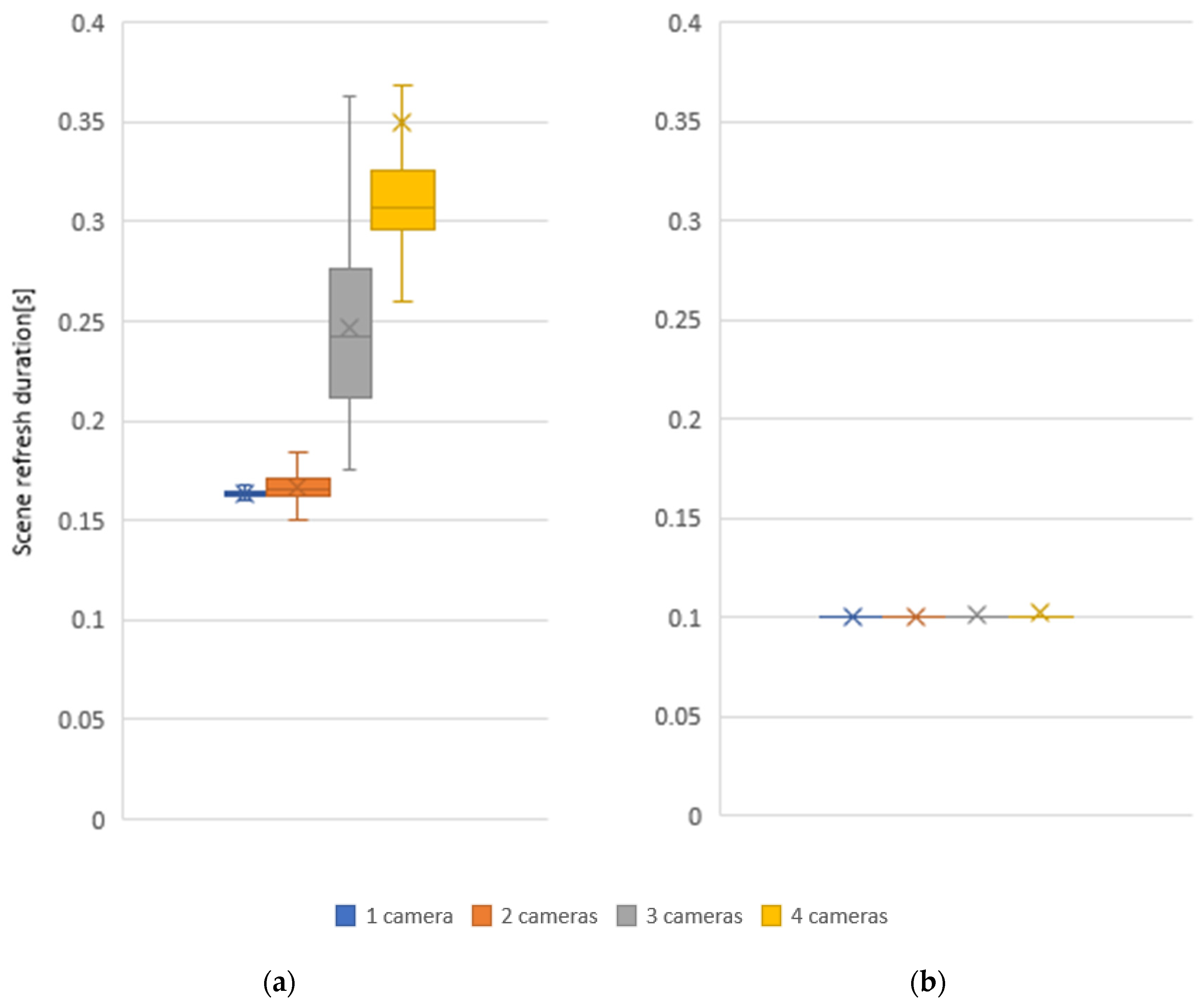
Subsequently, the effect of the number of cameras on scene refresh rate was measured for one, two, three, and four cameras in the workplace. The centralized system processes the camera data serially and does not allow the connecting of multiple cameras for a more detailed real-time mapping of the whole space since as the number of cameras increases, the time to recover the whole scene increases. In a distributed system, this problem does not arise since the computation is performed in parallel and is therefore not dependent on the number of cameras, see Figure 12.
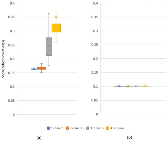
Figure 12.
Effect of the number of cameras on the scene refresh duration for 1280 × 720 camera resolution and voxel size 20 mm: (a) centralized; (b) distributed.
Scene refresh rate measurements based on the number of cameras have clearly shown that a system that filters data from each camera separately and sends the resulting data to the main device where all data are combined into a global voxel map is more efficient to use. The distributed system refresh rate is faster by 38.7% when using one camera, by 40.1% when using two cameras, 59.4% when using three cameras, and 71.5% when using four cameras. This ensures a more stable refresh rate of the whole scene even with larger numbers of sensors and reduces the network requirements as it does not need to send source data from cameras between devices.
Data sent over the network within a centralized system is sent in raw format (depth image), which equals the image width times height times the bit rate of the depth stream for each camera in the system. For example, when capturing at 640 × 480 resolution and a 32-bit depth image, then 9.8 Mbit of data needs to be transferred. For three cameras, this is therefore 29.4 Mbit/scene refresh. While in a distributed system, the data sent is based on the current scenario (nothing is sent if there are no undefined objects). When sending voxels (either an index in the grid or specific X,Y,Z coordinates), one can count 3 × 32 bits per voxel, whereas, in a normal scenario, the unit sends less than 100 voxels on average. Then, on average, 9.3 Kbit per camera can be counted, and with three cameras, it is only 27.9 Kbit.
To make a distributed system less efficient, the number of voxels sent would have to be higher than 1/3 of the number of pixels which is very unlikely with the current filtering.
Needed time may also be compared for implementing the system. In the case of a centralized system (MoveIt!), it was needed to manually change parts of the code responsible for placing cameras into the workspace (if no additional script was created for conducting this routine instead of us). That means if there was a need to change the number of cameras, there was a need to make changes in the code. On the other hand, while using a distributed system, it is needed just to place or remove a camera from the system with its computation unit to the change number of cameras. This makes this plug-and-play solution really user-friendly and much faster to implement. There is also an advantage in the case of system reachability. With a centralized system, reachability is limited by the length of the camera’s USB cable (which is around 2 m for securing fast data transfer) if only one computer is used. However, with distributed system, a 2 m USB cable should be always enough to reach the computing unit. Communication between the main device and computing units is addressed by a high-speed ethernet cable. This means there is a possibility of a greater spread of cameras in the workspace in the case of a distributed system.
4. Conclusions
Workspace monitoring is one of the essential elements of a workplace where a human has to interact with a robot. Reconstructing dynamic objects in the workplace can ensure safety for the operator and smooth operation of the workplace because the robot can react to changes in the free space for movement. The workplace reconstruction process is standard through packages in the Robotic Operation System (ROS). These packages are designed for universal use. However, this has the effect of centralizing the computing power into a single device. Such a solution is less suitable for processing large volumes of data from multiple sensors because the user does not have complete control over the computational processes.
Therefore, a new principle has been proposed that distributes the computational power among the individual devices. Each processing device allows filtering of the locally sensed data. The filtering is based on a 3D description of the workplace and the creation of a density camera depth map for each camera separately from their point of view. Filtering compares the actual depth map from the sensor and the calculated density depth map. The resulting data are information about undefined obstacles (arms, boxes, etc.). These obstacles are subsequently processed by noise filtering. The resulting data from the individual distributed devices are combined in the main computer (Algorithm 9), which produces an overall description of the entire sensed workspace.
This distributed sensing method was then verified and compared with the currently available centralized system (MoveIt!). The results show that both solutions are comparable across camera setups for different resolutions and voxel map sizes, but the main advantages of the distributed system are in the stable refresh rate of the whole scene when the number of sensors involved in the system changes. The measurements showed that when the number of cameras increased (1–4 cameras were measured), the scene refresh rate of the centralized system decreased substantially. In contrast, the distributed system maintained its scene refresh rate. Despite the fact that in a distributed system, the computation is performed in parallel on individual devices, when merging the data, there is a timestamp check to avoid unwanted effects (ghosts, broken data, etc.).
Based on the measurements, the system had shown to be able to maintain the workspace sensing rate even when the sensing parameters change. The essential parameter is the number of cameras, which significantly influences the refresh rate of the entire scene. The assumption that the distributed system is independent of the number of cameras has been proven, compared to the centralized system, which is slower with each additional camera added to the system. This assumption is especially evident when processing data from more than three cameras, where the data calculation from the whole scene is almost constant. If security in a given area should be ensured, the number of cameras will not be a limiting factor.
In terms of hardware, the only difference is in the final computing unit, which has higher computing power requirements in a centralized system than in a distributed system. The goal of this work was not to determine the exact computational power required for each system. The hardware in this work was selected based on previous experiences.
Despite the fact that filtering on distributed units runs on the CPU, the speed is comparable to the currently available solution in MoveIt!. Of course, this solution can be adapted to compute using a GPU, which can increase the speed; in general, this can be used on units that have graphic power available.
Future work could focus on noise elimination. In the current solution, voxel occupancy is judged based on the percentage of 3D points from a single camera. This approach could be more robust when using information from multiple cameras (e.g., two cameras detect a voxel as empty, and a third camera detects it as occupied). Further, the functionality of the system could be extended to automatically assign a size to each voxel based on the size and shape of the detected feature. This could lead to a reduction in the size of the total number of detected voxels. Consequently, it would be desirable to examine the trend of the ability to efficiently merge the processed camera image data. It is assumed that when processing tens of cameras (30–50 cameras), the rate of data merging should be constantly the same. This number of used cameras could be possibly used in the case of a huge workspace. However, the use of a higher number of cameras in the measurements was not considered, due to the insufficient budget to purchase a large number of cameras.
Author Contributions
Conceptualization, P.O., Z.B. and T.K.; methodology, P.O. and T.K.; software, P.O., T.K. and J.S.; validation, T.S. and Z.B.; formal analysis, S.G., D.H. and T.S.; investigation, P.O., D.H. and J.S.; resources, T.S. and S.G.; data curation, T.S., S.G. and J.S.; writing—original draft preparation, P.O., T.K., T.S. and D.H.; writing—review and editing, S.G., J.S. and D.H.; visualization, T.K. and P.O.; supervision, Z.B. and P.N.; project administration, Z.B. and P.N.; funding acquisition, P.N. All authors have read and agreed to the published version of the manuscript.
Funding
This work was supported by the Research Platform focused on Industry 4.0 and Robotics in the Ostrava Agglomeration project, project number CZ.02.1.01/0.0/0.0/17_049/0008425, within the Operational Program Research, Development, and Education. This article has been also supported by the specific research project SP2022/67 and financed by the state budget of the Czech Republic.
Institutional Review Board Statement
Not applicable.
Informed Consent Statement
Informed consent was obtained from all subjects involved in the study.
Data Availability Statement
The data presented in this study are available on request from the corresponding author. The data are not publicly available due to project restrictions.
Conflicts of Interest
The authors declare no conflict of interest. The funders had no role in the design of the study; in the collection, analyses, or interpretation of data; in the writing of the manuscript, or in the decision to publish the results.
References
- Feigin, M.; Bhandari, A.; Izadi, S.; Rhemann, C.; Schmidt, M.; Raskar, R. Resolving Multipath Interference in Kinect: An Inverse Problem Approach. IEEE Sens. J. 2016, 16, 3419–3427. [Google Scholar] [CrossRef]
- Bhandari, A.; Kadambi, A.; Whyte, R.; Barsi, C.; Feigin, M.; Dorrington, A.; Raskar, R. Resolving multipath interference in time-of-flight imaging via modulation frequency diversity and sparse regularization. Opt. Lett. 2014, 39, 1705–1708. [Google Scholar] [CrossRef]
- Naik, N.; Kadambi, A.; Rhemann, C.; Izadi, S.; Raskar, R.; Kang, S. A light transport model for mitigating multipath interference in TOF sensors. In Proceedings of the IEEE Conference on Computer Vision and Pattern Recognition (CVPR), Boston, MA, USA, 7–12 June 2015. [Google Scholar]
- Fanello, S.R.; Valentin, J.; Rhemann, C.; Kowdle, A.; Tankovich, V.; Davidson, P.; Izadi, S. UltraStereo: Efficient Learning-Based Matching for Active Stereo Systems. In Proceedings of the 2017 IEEE Conference on Computer Vision and Pattern Recognition (CVPR), Honolulu, HI, USA, 21–26 July 2017; pp. 6535–6544. [Google Scholar] [CrossRef]
- Fanello, S.R.; Rhemann, C.; Tankovich, V.; Kowdle, A.; Escolano, S.O.; Kim, D.; Izadi, S. HyperDepth: Learning Depth from Structured Light without Matching. In Proceedings of the 2016 IEEE Conference on Computer Vision and Pattern Recognition (CVPR), Las Vegas, NV, USA, 27–30 June 2016; pp. 5441–5450. [Google Scholar] [CrossRef]
- Zhang, Y.; Khamis, S.; Rhemann, C.; Valentin, J.; Kowdle, A.; Tankovich, V.; Schoenberg, M.; ShahramIzadi; Funkhouser, T.; Fanello, S. Activestereonet: End-to-end self-supervised learning for active stereo systems. In Proceedings of the European Conference on Computer Vision (ECCV), Munich, Germany, 7 October 2018; pp. 784–801. [Google Scholar] [CrossRef] [Green Version]
- Kumar Jha, V.; Grushko, S.; Mlotek, J.; Kot, T.; Krys, V.; Oscadal, P.; Bobovsky, Z. A depth image quality benchmark of three popular low-cost depth cameras. MM Sci. J. 2020, 2020, 4194–4200. [Google Scholar] [CrossRef]
- Duan, Y.; Chen, L.; Wang, Y.; Yang, M.; Qin, X.; He, S.; Jia, Y. A real-time system for 3D recovery of dynamic scene with multiple RGBD imagers. In Proceedings of the 2011 IEEE Computer Society Conference on Computer Vision and Pattern Recognition Workshops (CVPR Workshops), Colorado Springs, CO, USA, 20–25 June 2011; pp. 1–8. [Google Scholar] [CrossRef]
- Hayashi, S.; Igarashi, H. Touchless Information Provision and Facial Expression Training Using Kinect. In HCI International 2021—Posters, Proceedings of the 23rd HCI International Conference, HCII 2021, Virtual, 24–29 July 2021; Springer International Publishing: Cham, Switzerland, 2021. [Google Scholar] [CrossRef]
- Yang, K.; Peng, L.; Tong, L.; Liu, R.; Liu, B. An Assessment Method for Upper Limb Rehabilitation Training Using Kinect. In Proceedings of the 2018 IEEE 8th Annual International Conference on CYBER Technology in Automation, Control, and Intelligent Systems (CYBER), Tianjin, China, 19–23 July 2018. [Google Scholar] [CrossRef]
- Chulhee, B.; Lee, S. Object Recognition Using Deep Belief Nets with Spherical Signature Descriptor of 3DPoint Cloud Data for Extended Kalman Filter Based Simultaneous Localization and Mapping. In Proceedings of the 2018 15th International Conference on Ubiquitous Robots (UR), Honolulu, HI, USA, 26–30 June 2018. [Google Scholar] [CrossRef]
- Vysocky, A.; Novak, P. Human—Robot collaboration in industry. MM Sci. J. 2016, 9, 903–906. [Google Scholar] [CrossRef]
- Wang, L.; Gao, R.; Váncza, J.; Krüger, J.; Wang, X.V.; Makris, S.; Chryssolouris, G. Symbiotic human-robot collaborative assembly. CIRP Ann. 2019, 68, 701–726. [Google Scholar] [CrossRef] [Green Version]
- Messeri, C.; Masotti, G.; Zanchettin, A.M.; Rocco, P. Human-Robot Collaboration: Optimizing Stress and Productivity Based on Game Theory. IEEE Robot. Autom. Lett. 2021, 6, 8061–8068. [Google Scholar] [CrossRef]
- Chacón, A.; Ponsa, P.; Angulo, C. Usability Study through a Human-Robot Collaborative Workspace Experience. Designs 2021, 5, 35. [Google Scholar] [CrossRef]
- Grushko, S.; Vysocký, A.; Oščádal, P.; Vocetka, M.; Novák, P.; Bobovský, Z. Improved Mutual Understanding for Human-Robot Collaboration: Combining Human-Aware Motion Planning with Haptic Feedback Devices for Communicating Planned Trajectory. Sensors 2021, 21, 3673. [Google Scholar] [CrossRef]
- Grushko, S.; Vysocký, A.; Heczko, D.; Bobovský, Z. Intuitive Spatial Tactile Feedback for Better Awareness about Robot Trajectory during Human–Robot Collaboration. Sensors 2021, 21, 5748. [Google Scholar] [CrossRef] [PubMed]
- Moughlbay, A.A.; Herrero, H.; Pacheco, R.; Outón, J.L.; Sallé, D. Reliable Workspace Monitoring in Safe Human-Robot Environment. In International Joint Conference SOCO’16-CISIS’16-ICEUTE’16; Springer International Publishing: Berlin/Heidelberg, Germany, 2016; pp. 256–266. [Google Scholar] [CrossRef]
- Arents, J.; Abolins, V.; Judvaitis, J.; Vismanis, O.; Oraby, A.; Ozols, K. Human–Robot Collaboration Trends and Safety Aspects: A Systematic Review. J. Sens. Actuator Netw. 2021, 10, 48. [Google Scholar] [CrossRef]
- Chiriatti, G.; Palmieri, G.; Scoccia, C.; Palpacelli, M.C.; Callegari, M. Adaptive Obstacle Avoidance for a Class of Collaborative Robots. Machines 2021, 9, 113. [Google Scholar] [CrossRef]
- Brito, T.; Lima, J.; Costa, P.; Piardi, L. Dynamic Collision Avoidance System for a Manipulator Based on RGB-D Data. In Proceedings of the ROBOT 2017: Third Iberian Robotics Conference, Sevilla, Spain, 22–24 November 2017; Springer International Publishing: Cham, Switzerland, 2017; pp. 643–654. [Google Scholar] [CrossRef] [Green Version]
- Bogue, R. Detecting humans in the robot workspace. Ind. Robot. Int. J. 2017, 44, 689–694. [Google Scholar] [CrossRef]
- Munaro, M.; Lewis, C.; Chambers, D.; Hvass, P.; Menegatti, E. RGB-D Human Detection and Tracking for Industrial Environments. In Intelligent Autonomous Systems 13; Springer International Publishing: Cham, Switzerland, 2015; pp. 1655–1668. [Google Scholar] [CrossRef]
- Shu, X.; Yang, J.; Yan, R.; Song, Y. Expansion-Squeeze-Excitation Fusion Network for Elderly Activity Recognition. IEEE Trans. Circuits Syst. Video Technol. 2022. [Google Scholar] [CrossRef]
- Shu, X.; Qi, G.-J.; Tang, J.; Wang, J. Weakly-Shared Deep Transfer Networks for Heterogeneous-Domain Knowledge Propagation. In Proceedings of the 23rd ACM international conference on Multimedia, Brisbane, Australia, 26–30 October 2015; pp. 35–44. [Google Scholar] [CrossRef]
- Shu, X.; Zhang, L.; Qi, G.-J.; Liu, W.; Tang, J. Spatiotemporal Co-Attention Recurrent Neural Networks for Human-Skeleton Motion Prediction. IEEE Trans. Pattern Anal. Mach. Intell. 2022, 44, 3300–3315. [Google Scholar] [CrossRef]
- Tang, J.; Shu, X.; Yan, R.; Zhang, L. Coherence Constrained Graph LSTM for Group Activity Recognition. IEEE Trans. Pattern Anal. Mach. Intell. 2022, 44, 636–647. [Google Scholar] [CrossRef] [PubMed]
- Grushko, S.; Vysocky, A.; Jha, V.K.; Pastor, R.; Prada, E.; Mikova, L.; Bobovsky, Z. Tuning perception and motion planning parameters for moveit! Framework. MM Sci. J. 2020, 2020, 4154–4163. [Google Scholar] [CrossRef]
- Stanford Artificial Intelligence Laboratory. Robotic Operating System. 2018. Available online: https://www.ros.org (accessed on 15 June 2022).
- Cohen-Or, D.; Kaufman, A. Fundamentals of Surface Voxelization. Graph. Models Image Processing 1995, 57, 453–461. [Google Scholar] [CrossRef]
- Huczala, D.; Oščádal, P.; Spurný, T.; Vysocký, A.; Vocetka, M.; Bobovský, Z. Camera-Based Method for Identification of the Layout of a Robotic Workcell. Appl. Sci. 2020, 10, 7679. [Google Scholar] [CrossRef]
- Oščádal, P.; Heczko, D.; Vysocký, A.; Mlotek, J.; Novák, P.; Virgala, I.; Sukop, M.; Bobovský, Z. Improved Pose Estimation of Aruco Tags Using a Novel 3D Placement Strategy. Sensors 2020, 20, 4825. [Google Scholar] [CrossRef]
- Xu, Y.; Tong, X.; Stilla, U. Voxel-based representation of 3D point clouds: Methods, applications, and its potential use in the construction industry. Autom. Constr. 2021, 126, 103675. [Google Scholar] [CrossRef]
- Laine, S. A Topological Approach to Voxelization. Comput. Graph. Forum 2013, 32, 77–86. [Google Scholar] [CrossRef]
- Nourian, P.; Gonçalves, R.; Zlatanova, S.; Ohori, K.A.; Vu Vo, A. Voxelization algorithms for geospatial applications. MethodsX 2016, 3, 69–86. [Google Scholar] [CrossRef] [PubMed]
- Huczala, D.; Kot, T.; Pfurner, M.; Heczko, D.; Oščádal, P.; Mostýn, V. Initial Estimation of Kinematic Structure of a Robotic Manipulator as an Input for Its Synthesis. Appl. Sci. 2021, 11, 3548. [Google Scholar] [CrossRef]
- Jetson Nano Developer Kit. NVIDIA Developer. 14 April 2021. Available online: https://developer.nvidia.com/embedded/jetson-nano-developer-kit (accessed on 16 December 2021).
- Specification Lenovo IdeaPad Y910 80V1004CCK. MobileXfiles.Com. Available online: https://mobilexfiles.com/notebooks/lenovo/lenovo_ideapad_y910_80v1004cck/ (accessed on 16 December 2021).


Publisher’s Note: MDPI stays neutral with regard to jurisdictional claims in published maps and institutional affiliations. |
© 2022 by the authors. Licensee MDPI, Basel, Switzerland. This article is an open access article distributed under the terms and conditions of the Creative Commons Attribution (CC BY) license (https://creativecommons.org/licenses/by/4.0/).