
A Survey of Deep Learning-Based Image Restoration Methods for Enhancing Situational Awareness at Disaster Sites: The Cases of Rain, Snow and Haze

 , , , and
Abstract
:1. Introduction
- Conditions which degrade vision without fully obstructing it: such as rain, snow and haze. As objects or people are visible through such conditions both to the naked eye and RGB camera sensors, visual computing algorithms can be used to restore such images and improve visibility.
- Conditions which fully obstruct some or all parts of the field of view: such are total darkness, heavy smoke or dense dust. Such conditions beyond the capabilities of RGB sensors and computer vision algorithms to restore, necessitating other modalities and approaches, such as infrared sensors.
- We survey the research literature on the deraining, desnowing and dehazing methods that employ DL-based architectures. To the best of our knowledge, this work is the first survey of image restoration methods in adverse conditions for assisting FRs situational awareness.
- We provide a faceted taxonomy of the abovementioned image denoising methods in adverse weather conditions in terms of their technical attributes.
- We compare the existing algorithms in terms of quantitative metrics and processing time in order to decide the appropriateness of each method for the specific task of facilitating the FRs’ vision.
2. Datasets
2.1. Deraining Datasets

| Dataset | Synthetic (S)/Real (R) | Indoor (I)/Outdoor (O) | Pairs | Year |
|---|---|---|---|---|
| Rain12600 [17] | S | O | 14,000 | 2017 |
| Rain12000 [20] | S | O | 12,000 | 2018 |
| Rain1400 [17] | S | O | 1400 | 2017 |
| Rain800 [21] | R | O | 800 | 2020 |
| Rain12 [22] | S | O | 12 | 2016 |
| Test100 [21] | S | O | 100 | 2020 |
| Test1200 [20] | S | O | 1200 | 2018 |
| RainTrainH [20] | S | O | 1800 | 2018 |
| RainTrainL [20] | S | O | 200 | 2018 |
| Rain100H [23] | S | O | 100 | 2020 |
| Rain100L [23] | S | O | 100 | 2020 |
| Rain200H [24] | S | O | 2000 | 2017 |
| RID [25] | R | O | 2495 | 2019 |
| RIS [25] | R | O | 2048 | 2019 |
| DAWN/Rainy [26] | R | O | 200 | 2020 |
| NTURain [27] | S | O | 8 (videos) | 2018 |
| SPA-Data [28] | R | O | 29,500 | 2019 |
2.2. Desnowing Datasets
2.3. Dehazing Datasets
| Dataset | Synthetic (S)/Real (R) /Generated (G) | Indoor (I)/Outdoor (O) | Pairs | Year |
|---|---|---|---|---|
| FRIDA [33] | S | O | 72 | 2010 |
| FRIDA2 [34] | S | O | 264 | 2012 |
| CHIC [35] | G | I | 18 | 2016 |
| RESIDE [36] | S & R | I & O | 10,000+ | 2018 |
| D-HAZY [37] | S | I | 2016 | |
| I-HAZE [38] | G | I | 35 | 2018 |
| O-HAZE [39] | G | O | 45 | 2018 |
| DENSE-HAZE [40] | G | O | 35 | 2019 |
| NH-HAZE [41] | G | O | 55 | 2020 |
| HazeRD [44] | S | O | 70 | 2017 |
| BeDDE [45] | R | O | 2020 | |
| 4KID [46] | S | O | 10,000 | 2021 |
| REVIDE [47] | G | I | (videos) | 2021 |
3. A Review of the Deraining Literature
3.1. A Taxonomy of the DL-Based Single Image Deraining Methods
3.1.1. CNN-Based Deraining Methods
3.1.2. Different Learning Schemes for Deraining
3.1.3. Generative Models for Deraining
3.1.4. Attention Mechanisms for Deraining
3.1.5. Multi-Scale Based Deraining Methods
3.1.6. Recurrent Representations for Deraining
3.1.7. Data Fusion Strategies for Deraining
3.2. Multi-Image Deraining
3.2.1. Stereo-Based Methods for Deraining
3.2.2. Video-Based Methods for Deraining
| Category | Method | Model | Short Description | Year |
|---|---|---|---|---|
| CNN- based | DetailNet [17] | ACM | reduces mapping range; promotes HF details | 2017 |
| Residual-guide [55] | ACM | cascaded; residuals; coarse-to-fine | 2018 | |
| NLEDN [56] | ACM | end-to-end, non-locally-enhanced; spatial correlation | 2018 | |
| DID-MDN [20] | ACM | density-aware multi-stream densely connected CNN | 2018 | |
| DualCNN [57] | ACM | estimation of structures and details | 2018 | |
| Scale-free [54] | HRMLL | wavelet analysis | 2019 | |
| DMTNet [58] | ACM | symmetry reduces complexity; multidomain translation | 2021 | |
| UC-PFilt [60] | ACM | predictive kernels; removes residual rain traces | 2022 | |
| SAPNet [61] | N/A | PDUs; unsupervised background segmentation; perceptual loss | 2022 | |
| DDC [25] | SBM | decomposition and composition network; rain mask | 2019 | |
| DerainNet [48] | ACM | non-linear rainy-to-clear mapping | 2017 | |
| PCNet [62] | MRSL | learns joint features of rainy and clear content | 2021 | |
| Spatial Attention [28] | ACM | human supervision; global-to-local attention | 2019 | |
| memory encoder–decoder [59] | ACM | encoder–decoder architecture with memory | 2022 | |
| Attention | APAN [73] | ACM | multi-scale pyramid representation; attention | 2021 |
| IADN [71] | ACM | self-similarity of rain; mixed attention mechanism; fusion | 2020 | |
| DECAN [77] | ACM | detail-guided channel attention module identifies low-level features; background repair network | 2021 | |
| DAF-Net [72] | DRM | end-to-end model; depth-attentional features learning | 2019 | |
| SIR [78] | ACM | encoder–decoder embedding; layered LSTM | 2022 | |
| RadNet [75] | ACM/ Raindrop | restores raindrops and rainstreaks; handles single-type, superimposed-type or blended-type data | 2021 | |
| DARGNet [74] | HRM | dual-attention (spatial and channel) | 2021 | |
| task-adaptive attention [76] | N/A | task-adaptive, task-channel, task-operation attention | 2022 | |
| Generative models | DerainAttentionGAN [15] | ACM | uses Cycle-GAN; attention | 2022 |
| DerainCycleGAN [66] | ACM | CycleGAN transfer learning; unsupervised attention | 2021 | |
| RCA-cGAN [68] | ACM | rain streak characteristics; integration with cGAN | 2022 | |
| RainGAN [69] | Raindrop | raindrop removal as many-to-one translation | 2022 | |
| UD-GAN [13] | ACM | GAN; self-supervised constraints from intrinsic statistics | 2019 | |
| HeavyRainStorer [70] | HRM | 2-stage network; physics-based backbone; depth-guided GAN | 2019 | |
| ID-CGAN [21] | ACM | conditional GAN with additional constraint | 2020 | |
| AttGAN [65] | Raindrop | attentive GAN; learns rain structure | 2018 | |
| Multi-scale based | MSPFN [80] | N/A | streak correlations; multi-scale progressive fusion | 2020 |
| MRADN [83] | ACM | multi-scale residual aggregation; multi-scale context aggregation; multi-resolution feature extraction | 2021 | |
| LFDN [79] | N/A | encoder–decoder architecture; encoder with multi-scale analysis; decoder with feature distillation; module fusion | 2021 | |
| SphinxNet [84] | N/A | AEs for maximum spatial awareness; convolutional layers; skip concatenation connections | 2021 | |
| DFPGN [82] | ACM | cross-scale information merge; cross-layer feature fusion | 2021 | |
| GAGN [81] | ACM | context-wise; multi-scale analysis | 2022 | |
| UMRL [104] | ACM | UMRL network learns rain content at different scales | 2019 | |
| Different learning schemes | JORDER [23] | HRM | multi-task learning; priors on equation parameters | 2020 |
| FLUID [63] | N/A | few-shot; self-supervised; inpainting | 2022 | |
| Semi-supervised CNN [16] | ACM | adapts to unpaired data by training on paired data | 2019 | |
| Recurrent | PReNet [89] | ACM | repeated ResNet; recursive; multi-scale info extraction | 2019 |
| recurrent residual multi-scale [85] | MRSL | residual multi-scale pyramid; coarse-to-fine progressive rain removal; attention map; multi-scale kernel selection | 2022 | |
| Scale-aware [90] | HRM | multiple subnetworks handle range of rain characteristics | 2017 | |
| RESCAN [87] | Equation (A8) | contextual dilated network; squeeze-and-excitation block | 2018 | |
| Pyramid Derain [86] | ACM | Gaussian–Laplacian pyramid decomposition | 2019 | |
| DRN [93] | ACM | multi-stage residual network with two residual blocks | 2019 | |
| NCANet [88] | Equation (A10) | rain streaks as residuals sum; recurrent | 2022 | |
| PRRNet [91] | ACM | stereo; semantic segmentation; multi-view fusion | 2021 | |
| GTA-Net [105] | ACM | multi-stream coarse; single-stream fine | 2021 |
4. A Review of the Desnowing Literature
4.1. Related Work on the Desnowing Problem
4.1.1. CNN-Based Desnowing Methods
4.1.2. Generative Models for Desnowing
4.1.3. Multi-Scale Based Desnowing Methods
| Category | Method | Short Description | Year |
|---|---|---|---|
| CNN- based | HDCW-Net [30] | DTCWT analysis; recursively computes HF component; neural network reconstructs the last HF component | 2021 |
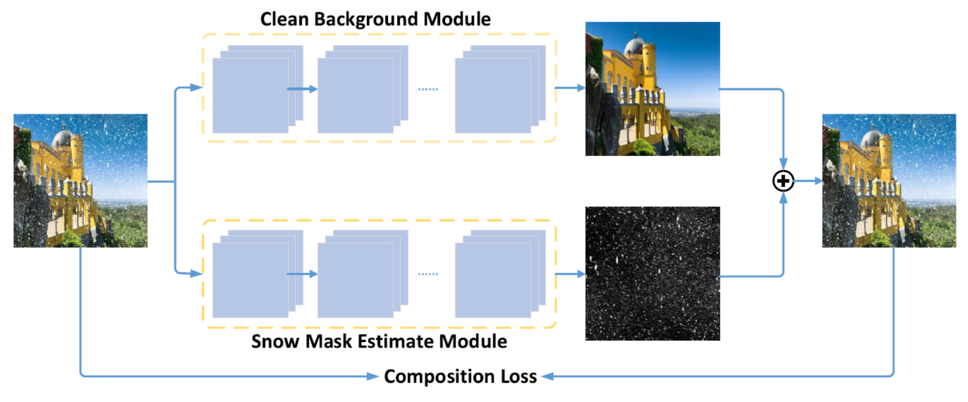
| Generative models | cGAN [106] | separates the background from snowy regions; uses compositional loss | 2019 |
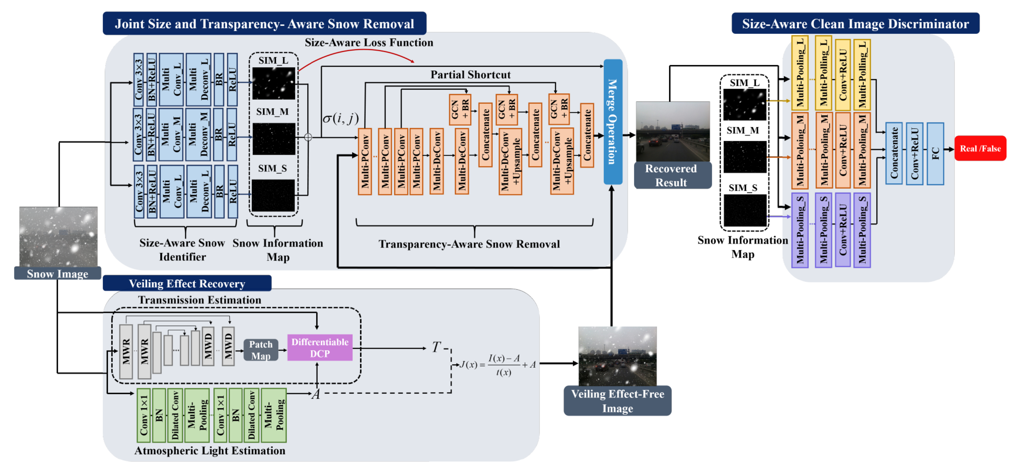
| JSTASR [32] | handles transparent/non-transparent snow particles; modified partial convolution; transparency aware; considers size and scale of snow particles | 2020 | |
| DesnowGAN [107] | DNN with top-down pathway and lateral cross-resolution connections; high-level and low-level spatial features; split-transform-merge topology reduces model size and computational cost; atrous spatial pyramid pooling for multi-scale and global receptive field | 2020 | |
| Multi-scale based | DesnowNet [29] | accurately corrects image content by estimating and restoring details in the image that are lost due to opaque snow particles | 2018 |
| MS-SDN [31] | multi-scale convolutional subnetwork extracts feature maps; stacked modified DenseNets for snowflakes detection and removal | 2019 | |
| DDMSNet [108] | multi-scale representation from pixel-level and feature-level input; multi-scale subnetwork are desnely connected; semantic and geometric priors; multistage analysis | 2021 |
5. A Review of the Dehazing Literature
5.1. A Taxonomy of the DL-Based Single Image Dehazing Methods
5.1.1. CNN-Based Dehazing Methods
5.1.2. Multi-Scale Based Dehazing Methods
5.1.3. Generative Models for Dehazing
5.1.4. Deep Reinforcement Learning for Dehazing
5.1.5. Knowledge Distillation/Transferring for Dehazing
5.1.6. Unsupervised/Semi-Supervised Learning for Dehazing
| Category | Method | Short Description | Year |
|---|---|---|---|
| CNN- based | Dehazenet [118] | 3-layer CNN, BReLU activation function | 2016 |
| AOD-Net [119] | lightweight, transformed ASM | 2017 | |
| Light-DehazeNet [120] | lightweight, transformed ASM, CVR module | 2021 | |
| FFA-Net [121] | attention-based feature fusion structure | 2020 | |
| AECR-Net [122] | AE-like, contrastive learning, feature fusion | 2021 | |
| Multi-scale based | MSFFA-Net [123] | multi-scale grid network, feature fusion | 2021 |
| GDNet [124] | 3 sub-processes, multi-scale grid network | 2019 | |
| MSCNN [125] | 2 nets: coarse- and fine-scale | 2016 | |
| MSCNN-HE [126] | 3 nets: coarse-, fine-scale and holistic edge guided | 2020 | |
| EMRA-Net [127] | 2 nets: TRA-CNN and EA-CNN | 2021 | |
| MSBDN [128] | dense feature fusion module, boosted decoder | 2020 | |
| FAMED-Net [129] | 3 encoders at different scales, fusion module | 2019 | |
| PGC [130] | PGC and DRB blocks | 2020 | |
| MSRA-Net [131] | CIELAB, 2 subnets (luminance, chrominance) | 2022 | |
| MSDFN [132] | depth-aware dehazing | 2021 | |
| DMPHN [133] | non-homogeneous haze, multi-patch architecture | 2020 | |
| TDN [134] | 3 subnets: coarse-, fine-scale and haze density | 2020 | |
| Jo et al. [135] | selective residual blocks | 2021 | |
| Generative models | DCPDN [136] | generator with 2 subnets, edge-preserving loss function | 2018 |
| DehazeGAN [137] | ASM-based GAN | 2018 | |
| DDN [138] | ASM-based, unpaired supervision | 2018 | |
| GFN [139] | fusion based, employs a hazy image and 3 derived inputs | 2018 | |
| EPDN [140] | multi-resolution generator, multi-scale discriminator, enhancer | 2019 | |
| cGAN [141] | cGAN with encoder–decoder architecture | 2018 | |
| Kan et al. [142] | cGAN, UR-Net as a generator, flexibility in image size | 2022 | |
| Cycle-Dehaze [143] | CycleGan based, unpaired supervision | 2018 | |
| CDNet [144] | CycleGan based, encoder–decoder architecture for the generator | 2019 | |
| Cycle-Defog2Refog [145] | 2 transformation paths with 2-stage mapping strategy in each | 2020 | |
| UCDN [146] | CycleGan based with a conditional disentangle network | 2020 | |
| DCA-CycleGAN [147] | generator with 2 subnets, 4 discriminators | 2022 | |
| Park et al. [148] | fusion of cGAN and CycleGAN | 2020 | |
| FD-GAN [109] | integration of HF and LF information in the discriminator | 2020 | |
| DW-GAN [149] | generator with a DWT and a Knowledge Adaptation Branch | 2021 | |
| TMS-GAN [150] | 2 subnets: a haze-generation and a haze-removal GAN | 2021 | |
| RL-based | Dehaze-RL [151] | actions: 11 dehazing algorithms, reward function: PSNR and SSIM | 2020 |
| DDRL [152] | depth-aware dehazing | 2020 | |
| Knowledge distillation/ transferring | KDDN [153] | teacher-student (dehazing) net | 2020 |
| Shao et al. [154] | domain adaptation using a bidirectional translation net | 2020 | |
| PSD [155] | domain adaptation by unsupervised fine-tuning (real domain) a pre-trained model (synthetic domain) | 2021 | |
| Yu et al. [156] | 2-branch net: transfer learning and current data fitting subnets | 2021 | |
| Unsupervised/ Semi- supervised | Golts et al. [157] | unsupervised, DCP loss | 2019 |
| Li et al. [158] | 2-branch: supervised and unsupervised subnets | 2019 | |
| RefineDNet [159] | 2-stage network: DCP and adversarial learning stages | 2021 | |
| YOLY [160] | self-supervised, 3 joint disentanglement subnetworks | 2021 |
5.2. Multi-Image Dehazing
6. Results
6.1. Quantitative Metrics
6.1.1. Peak Signal-to-Noise Ratio
6.1.2. Structural Similarity
6.2. Real-Time Performance Classification
6.3. Comparison of Models
6.3.1. Mathematical Background of Deraining
6.3.2. Comparison of Deraining Models
| Dataset | Method | PSNR ↑ | SSIM ↑ | FPS ↑ | Image Resolution | Classification |
|---|---|---|---|---|---|---|
| Test1200 | RESCAN [87] | 30.51 | 0.882 | 1.83 | non-real-time | |
| MSPFN [80] | 32.39 | 0.916 | 1.97 | non-real-time | ||
| PReNet [89] | 31.36 | 0.911 | 6.13 | near-real-time | ||
| IADN [71] | 32.29 | 0.916 | 7.57 | near-real-time | ||
| DDC [25] | 28.65 | 0.854 | 8.00 | near-real-time | ||
| DerainNet [48] | 23.38 | 0.835 | 13.51 | near-real-time | ||
| PCNet [167] | 32.03 | 0.913 | 16.12 | near-real-time | ||
| UMRL [104] | 21.15 | 0.770 | 20.00 | real-time | ||
| PCNet-fast [167] | 31.45 | 0.906 | 35.71 | real-time | ||
| LPNET [86] | 25.00 | 0.782 | 37.03 | real-time | ||
| Rain100L | JORDER [23] | 32.95 | 0.921 | 5.55 | near-real-time | |
| DDN [17] | 31.12 | 0.926 | 6.25 | near-real-time | ||
| ResGuideNet3 [55] | 30.79 | 0.939 | 16.66 | near-real-time |
6.3.3. Mathematical Background of Desnowing
6.3.4. Comparison of Desnowing Models
| Dataset | Method | PSNR ↑ | SSIM ↑ | FPS ↑ | Image Resolution | Classification |
|---|---|---|---|---|---|---|
| Snow-100K (overall) | DesnowNet [29] | 30.11 | 0.930 | 0.72 | non-real-time | |
| MS-SDN [31] | 29.25 | 0.936 | 2.38 | non-real-time | ||
| JSTASR [32] | 28.61 | 0.864 | 2.77 | non-real-time | ||
| DesnowGAN [107] | 28.18 | 0.912 | 33.33 | real-time |
6.3.5. Mathematical Background of Dehazing
6.3.6. Comparison of Dehazing Models
| Dataset | Method | PSNR ↑ | SSIM ↑ | FPS ↑ | Image Resolution | Classification |
|---|---|---|---|---|---|---|
| SOTS (RESIDE) | FFA-Net [121] | 36.39 | 0.988 | 0.57 | non-real-time | |
| Li et al. [158] | 24.44 | 0.890 | 0.89 | non-real-time | ||
| MSCNN-HE [126] | 21.56 | 0.860 | 1.20 | non-real-time | ||
| TDN [134] | 34.59 | 0.975 | 1.58 | near-real-time | ||
| DW-GAN [149] | 35.94 | 0.986 | 2.08 | near-real-time | ||
| Light-DehazeNet [120] | 28.39 | 0.948 | 2.38 | non-real-time | ||
| PGC [130] | 28.78 | 0.956 | 3.17 | near-real-time | ||
| MSFFA-Net [123] | 36.69 | 0.990 | 3.23 | near-real-time | ||
| DehazeNet [118] | 21.14 | 0.847 | 3.33 | near-real-time | ||
| EPDN [140] | 25.06 | 0.923 | 3.41 | near-real-time | ||
| Golts et al. [157] | 24.08 | 0.933 | 3.57 | near-real-time | ||
| GDNet [124] | 32.16 | 0.983 | 3.60 | near-real-time | ||
| MSCNN [125] | 17.57 | 0.810 | 3.85 | near-real-time | ||
| YOLY [160] | 19.41 | 0.832 | 4.76 | near-real-time | ||
| Yu et al. [156] | 36.61 | 0.991 | 11.24 | real-time | ||
| cGAN [141] | 26.63 | 0.942 | 19.23 | real-time | ||
| GFN [139] | 22.30 | 0.880 | 20.40 | real-time | ||
| DCPDN [136] | 19.39 | 0.650 | 23.98 | real-time | ||
| FD-GAN [109] | 23.15 | 0.920 | 65.00 | real-time | ||
| DMPHN [133] | 16.94 | 0.617 | 68.96 | real-time | ||
| FAMED-Net [129] | 25.00 | 0.917 | 86.20 | real-time | ||
| AOD-Net [119] | 19.06 | 0.850 | 232.56 | real-time |
7. Discussion and Conclusions
Author Contributions
Funding
Institutional Review Board Statement
Informed Consent Statement
Data Availability Statement
Conflicts of Interest
Abbreviations
| FR | First Responder |
| CV | Computer Vision |
| DL | Deep Learning |
| ML | Machine Learning |
| GPU | Graphics Processing Unit |
| CNN | Convolutional Neural Network |
| GAN | Generative Adversarial Network |
| AE | Autoencoder |
| HF | High Frequency |
| LF | Low Frequency |
| PDU | Progressive Dilated Unit |
| UBS | Unsupervised Background Segmentation |
| LSTM | Long Short-Term Memory |
| DNN | Deep Neural Network |
| DWT | Discrete Wavelet Transform |
| RL | Reinforcement Learning |
| PSNR | Peak-Signal-to-Noise Ratio |
| SSIM | Structural Similarity Index Measure |
| FPS | Frames Per Second |
Appendix A
Appendix A.1. Underlying Equations for Image Deraining
- Li et al. [90] model the observed rainy image O as a background layer B and a sequence of s rain streak layers . Each layer can model rain streaks of different characteristics (e.g., that of orientation and size). Their proposed model is known in the bibliography as Multiple Rain Streak Layers (MRSL) model and is shown in Equation (A1).
- The Heavy Rain Model (HRM) proposed by Yang et al. [24] is a convex combination of two quantities: (1) the underlying image modelled by a set of rain streak layers (s layers are assumed) and the background image B; (2) the global atmospheric light matrix A. The s rain-streak layers are able to capture the rain streaks with different characteristics. a is the atmospheric transmission parameter. Equation (A2) shows the HRM model.
- The model proposed by Xue et al. [54] assumes an image that is gamma corrected by an exponent . This image is linearly combined with the atmospheric light matrix A. This equation is similar to Equation (A2), except for the fact that the latter requires multiple rain streak layers . Their proposed model is known in the bibliography as Heavy Rain Model with Low Light (HRMLL) model and is shown in Equation (A3).
- Luo et al. [169] introduced the Screen Blend Model (SBM). Their model is inspired by the Equation (6), but a difference is that in the equation the last term is subtracted from the quantity . The entries in the matrix weigh each pixel entry by the relative importance of the background pixel value of the associated entry and the corresponding value in matrix S. The entries of this matrix can be regarded as the linear correlation among the signals. Therefore, each pixel intensity associated with an entry of O is reduced by the product of the values from B and S. The model is shown in Equation (A4).
- The equation Rain Model With Occlusion (RMO) by Liu et al. [170] is similar to the HRM, except that they mutually differ in the last term . In this term is a cancellation term that signifies whether the pixel at location belongs to the rain occluded region (Liu et al. [170] defines as “the region where the light transmittance of rain drop is low”) and matrix R is the rain reliance map.
- Equation (A9) by Yang et al. [23] is similar to Equation (6). The difference in the former equation is that the entries of matrix R are linearly combined with cancellation entries in a matrix S. When an entry of S is zero, the respective entry in matrix R is cancelled. In turn, when an entry of S equals 1, then the respective intensity value in the entry of R is promoted. Hence, the term O in is similar to the equation , but a difference is that the entries in where the respective entry in S is zero are cancelled. When each entry in S equals 1, the respective entry in O is modelled as .
- The Raindrop Equation (A11) proposed by Qian et al. [65] models the relationship between the colored image I, a binary mask matrix M with zero-or-one entries, the clean background image B and the matrix R. Matrix R represents the raindrop information, which is a combination of the background information and the light reflected by the environment through the raindrops.
Appendix A.2. Loss Functions Employed in the Deraining Problem
Appendix A.3. Loss Functions Used by Desnowing Methods
References
- Asami, K.; Shono Fujita, K.H.; Hatayama, M. Data Augmentation with Synthesized Damaged Roof Images Generated by GAN. In Proceedings of the ISCRAM 2022 Conference Proceedings, 19th International Conference on Information Systems for Crisis Response and Management, Tarbes, France, 7–9 November 2022. [Google Scholar]
- Algiriyage, N.; Prasanna, R.; Doyle, E.E.; Stock, K.; Johnston, D. Traffic Flow Estimation based on Deep Learning for Emergency Traffic Management using CCTV Images. In Proceedings of the 17th International Conference on Information Systems for Crisis Response and Management, Blacksburg, VA, USA, 24–27 May 2020; pp. 100–109. [Google Scholar]
- Algiriyage, N.; Prasanna, R.; Doyle, E.E.; Stock, K.; Johnston, D.; Punchihewa, M.; Jayawardhana, S. Towards Real-time Traffic Flow Estimation using YOLO and SORT from Surveillance Video Footage. In Proceedings of the 18th International Conference on Information Systems for Crisis Response and Management, Blacksburg, VA, USA, 23–26 May 2021. [Google Scholar]
- Correia, H.R.; da Costa Rubim, I.; Dias, A.F.; França, J.B.; Borges, M.R. Drones to the Rescue: A Support Solution for Emergency Response. In Proceedings of the ISCRAM 2020 Conference Proceedings, 17th International Conference on Information Systems for Crisis Response and Management, Blacksburg, VA, USA, 24–27 May 2020. [Google Scholar]
- Sainidis, D.; Tsiakmakis, D.; Konstantoudakis, K.; Albanis, G.; Dimou, A.; Daras, P. Single-handed gesture UAV control and video feed AR visualization for first responders. In Proceedings of the International Conference on Information Systems for Crisis Response and Management (ISCRAM), Blacksburg, VA, USA, 23–26 May 2021; pp. 23–26. [Google Scholar]
- Zaffaroni, M.; Rossi, C. Water Segmentation with Deep Learning Models for Flood Detection and Monitoring. In Proceedings of the Conference on Information Systems for Crisis Response and Management (ISCRAM 2020), Blacksburg, VA, USA, 24–27 May 2020; pp. 24–27. [Google Scholar]
- Rothmeier, T.; Huber, W. Performance Evaluation of Object Detection Algorithms under Adverse Weather Conditions. In Proceedings of the International Conference on Intelligent Transport Systems, Indianapolis, IN, USA, 20–23 September 2020; Springer: Berlin/Heidelberg, Germany, 2020; pp. 211–222. [Google Scholar]
- Pfeuffer, A.; Dietmayer, K. Optimal Sensor Data Fusion Architecture for Object Detection in Adverse Weather Conditions. In Proceedings of the 2018 21st International Conference on Information Fusion (FUSION), Cambridge, UK, 10–13 July 2018; pp. 1–8. [Google Scholar] [CrossRef] [Green Version]
- Hasirlioglu, S.; Riener, A. Challenges in object detection under rainy weather conditions. In Proceedings of the First International Conference on Intelligent Transport Systems, Funchal, Portugal, 16–18 March 2018; Springer: Berlin/Heidelberg, Germany; pp. 53–65. [Google Scholar]
- Chaturvedi, S.S.; Zhang, L.; Yuan, X. Pay “Attention” to Adverse Weather: Weather-aware Attention-based Object Detection. arXiv 2022, arXiv:2204.10803. [Google Scholar]
- Morrison, K.; Choong, Y.Y.; Dawkins, S.; Prettyman, S.S. Communication Technology Problems and Needs of Rural First Responders. Public Law 2012, 112, 96. [Google Scholar]
- Su, J.; Xu, B.; Yin, H. A survey of deep learning approaches to image restoration. Neurocomputing 2022, 487, 46–65. [Google Scholar] [CrossRef]
- Jin, X.; Chen, Z.; Lin, J.; Chen, Z.; Zhou, W. Unsupervised single image deraining with self-supervised constraints. In Proceedings of the 2019 IEEE International Conference on Image Processing (ICIP), Taipei, Taiwan, 22–25 September 2019; pp. 2761–2765. [Google Scholar]
- Yadav, S.; Mehra, A.; Rohmetra, H.; Ratnakumar, R.; Narang, P. DerainGAN: Single image deraining using wasserstein GAN. Multimed. Tools Appl. 2021, 80, 36491–36507. [Google Scholar] [CrossRef]
- Guo, Z.; Hou, M.; Sima, M.; Feng, Z. DerainAttentionGAN: Unsupervised single-image deraining using attention-guided generative adversarial networks. Signal Image Video Process. 2022, 16, 185–192. [Google Scholar] [CrossRef]
- Wei, W.; Meng, D.; Zhao, Q.; Xu, Z.; Wu, Y. Semi-Supervised Transfer Learning for Image Rain Removal. In Proceedings of the IEEE/CVF Conference on Computer Vision and Pattern Recognition (CVPR), Long Beach, CA, USA, 15–20 June 2019. [Google Scholar]
- Fu, X.; Huang, J.; Zeng, D.; Huang, Y.; Ding, X.; Paisley, J. Removing Rain From Single Images via a Deep Detail Network. In Proceedings of the IEEE Conference on Computer Vision and Pattern Recognition (CVPR), Honolulu, HI, USA, 21–26 July 2017. [Google Scholar]
- Schaefer, G.; Stich, M. UCID: An uncompressed color image database. In Storage and Retrieval Methods and Applications for Multimedia 2004; International Society for Optics and Photonics: Bellingham, WA, USA, 2003; Volume 5307, pp. 472–480. [Google Scholar]
- Martin, D.R.; Fowlkes, C.C.; Malik, J. Learning to detect natural image boundaries using local brightness, color, and texture cues. IEEE Trans. Pattern Anal. Mach. Intell. 2004, 26, 530–549. [Google Scholar] [CrossRef]
- Zhang, H.; Patel, V.M. Density-Aware Single Image De-Raining Using a Multi-Stream Dense Network. In Proceedings of the IEEE Conference on Computer Vision and Pattern Recognition (CVPR), Salt Lake City, UT, USA, 18–23 June 2018. [Google Scholar]
- Zhang, H.; Sindagi, V.; Patel, V.M. Image De-Raining Using a Conditional Generative Adversarial Network. IEEE Trans. Circuits Syst. Video Technol. 2020, 30, 3943–3956. [Google Scholar] [CrossRef] [Green Version]
- Li, Y.; Tan, R.T.; Guo, X.; Lu, J.; Brown, M.S. Rain streak removal using layer priors. In Proceedings of the IEEE Conference on Computer Vision and Pattern Recognition, Las Vegas, NV, USA, 27–30 June 2016; pp. 2736–2744. [Google Scholar]
- Yang, W.; Tan, R.T.; Feng, J.; Guo, Z.; Yan, S.; Liu, J. Joint Rain Detection and Removal from a Single Image with Contextualized Deep Networks. IEEE Trans. Pattern Anal. Mach. Intell. 2020, 42, 1377–1393. [Google Scholar] [CrossRef]
- Yang, W.; Tan, R.T.; Feng, J.; Liu, J.; Guo, Z.; Yan, S. Deep Joint Rain Detection and Removal From a Single Image. In Proceedings of the IEEE Conference on Computer Vision and Pattern Recognition (CVPR), Honolulu, HI, USA, 21–26 July 2017. [Google Scholar]
- Li, S.; Ren, W.; Zhang, J.; Yu, J.; Guo, X. Single image rain removal via a deep decomposition–composition network. Comput. Vis. Image Underst. 2019, 186, 48–57. [Google Scholar] [CrossRef]
- Kenk, M.A.; Hassaballah, M. DAWN: Vehicle detection in adverse weather nature dataset. arXiv 2020, arXiv:2008.05402. [Google Scholar]
- Chen, J.; Tan, C.H.; Hou, J.; Chau, L.P.; Li, H. Robust video content alignment and compensation for rain removal in a cnn framework. In Proceedings of the IEEE Conference on Computer Vision and Pattern Recognition, Salt Lake City, UT, USA, 18–23 June 2018; pp. 6286–6295. [Google Scholar]
- Wang, T.; Yang, X.; Xu, K.; Chen, S.; Zhang, Q.; Lau, R.W. Spatial attentive single-image deraining with a high quality real rain dataset. In Proceedings of the IEEE/CVF Conference on Computer Vision and Pattern Recognition, Long Beach, CA, USA, 16–17 June 2019; pp. 12270–12279. [Google Scholar]
- Liu, Y.F.; Jaw, D.W.; Huang, S.C.; Hwang, J.N. DesnowNet: Context-aware deep network for snow removal. IEEE Trans. Image Process. 2018, 27, 3064–3073. [Google Scholar] [CrossRef] [PubMed] [Green Version]
- Chen, W.T.; Fang, H.Y.; Hsieh, C.L.; Tsai, C.C.; Chen, I.; Ding, J.J.; Kuo, S.Y. ALL Snow Removed: Single Image Desnowing Algorithm Using Hierarchical Dual-Tree Complex Wavelet Representation and Contradict Channel Loss. In Proceedings of the IEEE/CVF International Conference on Computer Vision, Montreal, BC, Canada, 11–17 October 2021; pp. 4196–4205. [Google Scholar]
- Li, P.; Yun, M.; Tian, J.; Tang, Y.; Wang, G.; Wu, C. Stacked dense networks for single-image snow removal. Neurocomputing 2019, 367, 152–163. [Google Scholar] [CrossRef]
- Chen, W.T.; Fang, H.Y.; Ding, J.J.; Tsai, C.C.; Kuo, S.Y. JSTASR: Joint size and transparency-aware snow removal algorithm based on modified partial convolution and veiling effect removal. In European Conference on Computer Vision; Springer: Berlin/Heidelberg, Germany, 2020; pp. 754–770. [Google Scholar]
- Tarel, J.P.; Hautiere, N.; Cord, A.; Gruyer, D.; Halmaoui, H. Improved visibility of road scene images under heterogeneous fog. In Proceedings of the 2010 IEEE Intelligent Vehicles Symposium, La Jolla, CA, USA, 21–24 June 2010; pp. 478–485. [Google Scholar]
- Tarel, J.P.; Hautiere, N.; Caraffa, L.; Cord, A.; Halmaoui, H.; Gruyer, D. Vision enhancement in homogeneous and heterogeneous fog. IEEE Intell. Transp. Syst. Mag. 2012, 4, 6–20. [Google Scholar] [CrossRef] [Green Version]
- El Khoury, J.; Thomas, J.B.; Mansouri, A.A. A color image database for haze model and dehazing methods evaluation. In International Conference on Image and Signal Processing; Springer: Berlin/Heidelberg, Germany, 2016; pp. 109–117. [Google Scholar]
- Li, B.; Ren, W.; Fu, D.; Tao, D.; Feng, D.; Zeng, W.; Wang, Z. Benchmarking single-image dehazing and beyond. IEEE Trans. Image Process. 2018, 28, 492–505. [Google Scholar] [CrossRef] [PubMed] [Green Version]
- Ancuti, C.; Ancuti, C.O.; De Vleeschouwer, C. D-hazy: A dataset to evaluate quantitatively dehazing algorithms. In Proceedings of the 2016 IEEE international conference on image processing (ICIP), Phoenix, AZ, USA, 25–28 September 2016; pp. 2226–2230. [Google Scholar]
- Ancuti, C.; Ancuti, C.O.; Timofte, R.; De Vleeschouwer, C. I-HAZE: A dehazing benchmark with real hazy and haze-free indoor images. In International Conference on Advanced Concepts for Intelligent Vision Systems; Springer: Berlin/Heidelberg, Germany, 2018; pp. 620–631. [Google Scholar]
- Ancuti, C.O.; Ancuti, C.; Timofte, R.; De Vleeschouwer, C. O-haze: A dehazing benchmark with real hazy and haze-free outdoor images. In Proceedings of the IEEE Conference on Computer Vision and Pattern Recognition Workshops, Salt Lake City, UT, USA, 18–23 June 2018; pp. 754–762. [Google Scholar]
- Ancuti, C.O.; Ancuti, C.; Sbert, M.; Timofte, R. Dense-haze: A benchmark for image dehazing with dense-haze and haze-free images. In Proceedings of the 2019 IEEE International Conference on Image Processing (ICIP), Taipei, Taiwan, 22–25 September 2019; pp. 1014–1018. [Google Scholar]
- Ancuti, C.O.; Ancuti, C.; Timofte, R. NH-HAZE: An image dehazing benchmark with non-homogeneous hazy and haze-free images. In Proceedings of the IEEE/CVF Conference on Computer Vision and Pattern Recognition Workshops, Seattle, WA, USA, 14–19 June 2020; pp. 444–445. [Google Scholar]
- Scharstein, D.; Hirschmüller, H.; Kitajima, Y.; Krathwohl, G.; Nešić, N.; Wang, X.; Westling, P. High-resolution stereo datasets with subpixel-accurate ground truth. In German Conference on Pattern Recognition; Springer: Berlin/Heidelberg, Germany, 2014; pp. 31–42. [Google Scholar]
- Silberman, N.; Hoiem, D.; Kohli, P.; Fergus, R. Indoor segmentation and support inference from rgbd images. In European Conference on Computer Vision; Springer: Berlin/Heidelberg, Germany, 2012; pp. 746–760. [Google Scholar]
- Zhang, Y.; Ding, L.; Sharma, G. Hazerd: An outdoor scene dataset and benchmark for single image dehazing. In Proceedings of the 2017 IEEE International Conference on Image Processing (ICIP), Beijing, China, 17–20 September 2017; pp. 3205–3209. [Google Scholar]
- Zhao, S.; Zhang, L.; Huang, S.; Shen, Y.; Zhao, S. Dehazing evaluation: Real-world benchmark datasets, criteria, and baselines. IEEE Trans. Image Process. 2020, 29, 6947–6962. [Google Scholar] [CrossRef]
- Zheng, Z.; Ren, W.; Cao, X.; Hu, X.; Wang, T.; Song, F.; Jia, X. Ultra-high-definition image dehazing via multi-guided bilateral learning. In Proceedings of the 2021 IEEE/CVF Conference on Computer Vision and Pattern Recognition (CVPR), Nashville, TN, USA, 20–25 June 2021; pp. 16180–16189. [Google Scholar]
- Zhang, X.; Dong, H.; Pan, J.; Zhu, C.; Tai, Y.; Wang, C.; Li, J.; Huang, F.; Wang, F. Learning to restore hazy video: A new real-world dataset and a new method. In Proceedings of the IEEE/CVF Conference on Computer Vision and Pattern Recognition, Nashville, TN, USA, 20–25 June 2021; pp. 9239–9248. [Google Scholar]
- Fu, X.; Huang, J.; Ding, X.; Liao, Y.; Paisley, J. Clearing the skies: A deep network architecture for single-image rain removal. IEEE Trans. Image Process. 2017, 26, 2944–2956. [Google Scholar] [CrossRef] [Green Version]
- Li, S.; Ren, W.; Wang, F.; Araujo, I.B.; Tokuda, E.K.; Junior, R.H.; Cesar, R.M., Jr.; Wang, Z.; Cao, X. A Comprehensive Benchmark Analysis of Single Image Deraining: Current Challenges and Future Perspectives. Int. J. Comput. Vis. 2021, 129, 1301–1322. [Google Scholar] [CrossRef]
- Wang, H.; Wu, Y.; Li, M.; Zhao, Q.; Meng, D. Survey on rain removal from videos or a single image. Sci. China Inf. Sci. 2021, 65, 111101. [Google Scholar] [CrossRef]
- Du, S.; Liu, Y.; Zhao, M.; Shi, Z.; You, Z.; Li, J. A comprehensive survey: Image deraining and stereo-matching task-driven performance analysis. IET Image Process. 2022, 16, 11–28. [Google Scholar] [CrossRef]
- Hnewa, M.; Radha, H. Object Detection Under Rainy Conditions for Autonomous Vehicles: A Review of State-of-the-Art and Emerging Techniques. IEEE Signal Process. Mag. 2021, 38, 53–67. [Google Scholar] [CrossRef]
- Yang, W.; Tan, R.T.; Wang, S.; Fang, Y.; Liu, J. Single Image Deraining: From Model-Based to Data-Driven and Beyond. IEEE Trans. Pattern Anal. Mach. Intell. 2021, 43, 4059–4077. [Google Scholar] [CrossRef] [PubMed]
- Yang, W.; Liu, J.; Yang, S.; Guo, Z. Scale-free single image deraining via visibility-enhanced recurrent wavelet learning. IEEE Trans. Image Process. 2019, 28, 2948–2961. [Google Scholar] [CrossRef] [PubMed]
- Fan, Z.; Wu, H.; Fu, X.; Huang, Y.; Ding, X. Residual-guide network for single image deraining. In Proceedings of the 26th ACM International Conference on Multimedia, Seoul, Korea, 22–26 October 2018; pp. 1751–1759. [Google Scholar]
- Li, G.; He, X.; Zhang, W.; Chang, H.; Dong, L.; Lin, L. Non-locally enhanced encoder-decoder network for single image de-raining. In Proceedings of the 26th ACM International Conference on Multimedia, Seoul, Korea, 22–26 October 2018; pp. 1056–1064. [Google Scholar]
- Pan, J.; Liu, S.; Sun, D.; Zhang, J.; Liu, Y.; Ren, J.; Li, Z.; Tang, J.; Lu, H.; Tai, Y.W.; et al. Learning dual convolutional neural networks for low-level vision. In Proceedings of the IEEE Conference on Computer Vision and Pattern Recognition, Salt Lake City, UT, USA, 18–23 June 2018; pp. 3070–3079. [Google Scholar]
- Huang, Z.; Zhang, J. Dynamic Multi-Domain Translation Network for Single Image Deraining. In Proceedings of the 2021 IEEE International Conference on Image Processing (ICIP), Anchorage, AK, USA, 19–22 September 2021; pp. 1754–1758. [Google Scholar] [CrossRef]
- Cho, J.; Kim, S.; Sohn, K. Memory-guided Image De-raining Using Time-Lapse Data. arXiv 2022, arXiv:2201.01883. [Google Scholar] [CrossRef] [PubMed]
- Guo, Q.; Sun, J.; Juefei-Xu, F.; Ma, L.; Lin, D.; Feng, W.; Wang, S. Uncertainty-Aware Cascaded Dilation Filtering for High-Efficiency Deraining. arXiv 2022, arXiv:2201.02366. [Google Scholar]
- Zheng, S.; Lu, C.; Wu, Y.; Gupta, G. SAPNet: Segmentation-Aware Progressive Network for Perceptual Contrastive Deraining. In Proceedings of the IEEE/CVF Winter Conference on Applications of Computer Vision, Waikoloa, HI, USA, 4–8 January 2022; pp. 52–62. [Google Scholar]
- Jiang, K.; Wang, Z.; Yi, P.; Chen, C.; Wang, Z.; Lin, C.W. PCNET: Progressive Coupled Network for Real-Time Image Deraining. In Proceedings of the 2021 IEEE International Conference on Image Processing (ICIP), Anchorage, AK, USA, 19–22 September 2021; pp. 1759–1763. [Google Scholar]
- Rai, S.N.; Saluja, R.; Arora, C.; Balasubramanian, V.N.; Subramanian, A.; Jawahar, C. FLUID: Few-Shot Self-Supervised Image Deraining. In Proceedings of the IEEE/CVF Winter Conference on Applications of Computer Vision, Waikoloa, HI, USA, 4–8 January 2022; pp. 3077–3086. [Google Scholar]
- Goodfellow, I.; Pouget-Abadie, J.; Mirza, M.; Xu, B.; Warde-Farley, D.; Ozair, S.; Courville, A.; Bengio, Y. Generative adversarial nets. In Proceedings of the Advances in Neural Information Processing Systems 27, Montreal, QC, Canada, 8–13 December 2014. [Google Scholar]
- Qian, R.; Tan, R.T.; Yang, W.; Su, J.; Liu, J. Attentive Generative Adversarial Network for Raindrop Removal From a Single Image. In Proceedings of the IEEE Conference on Computer Vision and Pattern Recognition (CVPR), Salt Lake City, UT, USA, 18–23 June 2018. [Google Scholar]
- Wei, Y.; Zhang, Z.; Wang, Y.; Xu, M.; Yang, Y.; Yan, S.; Wang, M. DerainCycleGAN: Rain attentive CycleGAN for single image deraining and rainmaking. IEEE Trans. Image Process. 2021, 30, 4788–4801. [Google Scholar] [CrossRef]
- Zhu, J.Y.; Park, T.; Isola, P.; Efros, A.A. Unpaired Image-to-Image Translation using Cycle-Consistent Adversarial Networks. In Proceedings of the 2017 IEEE International Conference Computer Vision (ICCV), Venice, Italy, 22–29 October 2017. [Google Scholar]
- Yang, F.; Ren, J.; Lu, Z.; Zhang, J.; Zhang, Q. Rain-component-aware capsule-GAN for single image de-raining. Pattern Recognit. 2022, 123, 108377. [Google Scholar] [CrossRef]
- Yan, X.; Loke, Y.R. RainGAN: Unsupervised Raindrop Removal via Decomposition and Composition. In Proceedings of the IEEE/CVF Winter Conference on Applications of Computer Vision (WACV) Workshops, Waikoloa, HI, USA, 4–8 January 2022; pp. 14–23. [Google Scholar]
- Li, R.; Cheong, L.F.; Tan, R.T. Heavy rain image restoration: Integrating physics model and conditional adversarial learning. In Proceedings of the IEEE/CVF Conference on Computer Vision and Pattern Recognition, Long Beach, CA, USA, 15–20 June 2019; pp. 1633–1642. [Google Scholar]
- Jiang, K.; Wang, Z.; Yi, P.; Chen, C.; Han, Z.; Lu, T.; Huang, B.; Jiang, J. Decomposition makes better rain removal: An improved attention-guided deraining network. IEEE Trans. Circuits Syst. Video Technol. 2020, 31, 3981–3995. [Google Scholar] [CrossRef]
- Hu, X.; Fu, C.W.; Zhu, L.; Heng, P.A. Depth-attentional features for single-image rain removal. In Proceedings of the IEEE/CVF Conference on Computer Vision and Pattern Recognition, Long Beach, CA, USA, 15–20 June 2019; pp. 8022–8031. [Google Scholar]
- Wang, Q.; Sun, G.; Fan, H.; Li, W.; Tang, Y. APAN: Across-scale Progressive Attention Network for Single Image Deraining. IEEE Signal Process. Lett. 2021, 29, 159–163. [Google Scholar] [CrossRef]
- Zhang, H.; Xie, Q.; Lu, B.; Gai, S. Dual attention residual group networks for single image deraining. Digit. Signal Process. 2021, 116, 103106. [Google Scholar] [CrossRef]
- Wei, Y.; Zhang, Z.; Xu, M.; Hong, R.; Fan, J.; Yan, S. Robust Attention Deraining Network for Synchronous Rain Streaks and Raindrops Removal. TechRxiv 2021. [Google Scholar] [CrossRef]
- Zhou, J.; Leong, C.; Lin, M.; Liao, W.; Li, C. Task Adaptive Network for Image Restoration with Combined Degradation Factors. In Proceedings of the IEEE/CVF Winter Conference on Applications of Computer Vision (WACV) Workshops, Waikoloa, HI, USA, 4–8 January 2022; pp. 1–8. [Google Scholar]
- Lin, X.; Huang, Q.; Huang, W.; Tan, X.; Fang, M.; Ma, L. Single Image Deraining via detail-guided Efficient Channel Attention Network. Comput. Graph. 2021, 97, 117–125. [Google Scholar] [CrossRef]
- Li, Y.; Monno, Y.; Okutomi, M. Single Image Deraining Network with Rain Embedding Consistency and Layered LSTM. In Proceedings of the IEEE/CVF Winter Conference on Applications of Computer Vision, Waikoloa, HI, USA, 4–8 January 2022; pp. 4060–4069. [Google Scholar]
- Zhang, Y.; Liu, Y.; Li, Q.; Wang, J.; Qi, M.; Sun, H.; Xu, H.; Kong, J. A Lightweight Fusion Distillation Network for Image Deblurring and Deraining. Sensors 2021, 21, 5312. [Google Scholar] [CrossRef] [PubMed]
- Jiang, K.; Wang, Z.; Yi, P.; Chen, C.; Huang, B.; Luo, Y.; Ma, J.; Jiang, J. Multi-Scale Progressive Fusion Network for Single Image Deraining. In Proceedings of the IEEE/CVF Conference on Computer Vision and Pattern Recognition (CVPR), Seattle, WA, USA, 13–19 June 2020. [Google Scholar]
- Fu, B.; Jiang, Y.; Wang, H.; Wang, Q.; Gao, Q.; Tang, Y. Context-wise attention-guided network for single image deraining. Electron. Lett. 2022, 58, 148–150. [Google Scholar] [CrossRef]
- Wang, Z.; Wang, C.; Su, Z.; Chen, J. Dense Feature Pyramid Grids Network for Single Image Deraining. In Proceedings of the ICASSP 2021–2021 IEEE International Conference on Acoustics, Speech and Signal Processing (ICASSP), Toronto, ON, Canada, 6–11 June 2021; pp. 2025–2029. [Google Scholar] [CrossRef]
- Yamamichi, K.; Han, X.H. Multi-scale Residual Aggregation Deraining Network with Spatial Context-aware Pooling and Activation. In Proceedings of the British Machine Vision Conference, Virtual, 23–25 November 2021. [Google Scholar]
- Jasuja, C.; Gupta, H.; Gupta, D.; Parihar, A.S. SphinxNet-A Lightweight Network for Single Image Deraining. In Proceedings of the 2021 International Conference on Intelligent Technologies (CONIT), Hubli, India, 25–27 June 2021; pp. 1–6. [Google Scholar]
- Zheng, Y.; Yu, X.; Liu, M.; Zhang, S. Single-image deraining via recurrent residual multiscale networks. IEEE Trans. Neural Netw. Learn. Syst. 2022, 33, 1310–1323. [Google Scholar] [CrossRef] [PubMed]
- Fu, X.; Liang, B.; Huang, Y.; Ding, X.; Paisley, J. Lightweight pyramid networks for image deraining. IEEE Trans. Neural Netw. Learn. Syst. 2019, 31, 1794–1807. [Google Scholar] [CrossRef] [Green Version]
- Li, X.; Wu, J.; Lin, Z.; Liu, H.; Zha, H. Rescan: Recurrent squeeze-and-excitation context aggregation net. In Proceedings of the European Conference on Computer Vision, Munich, Germany, 8–14 September 2018. [Google Scholar]
- Su, Z.; Zhang, Y.; Zhang, X.P.; Qi, F. Non-local channel aggregation network for single image rain removal. Neurocomputing 2022, 469, 261–272. [Google Scholar] [CrossRef]
- Ren, D.; Zuo, W.; Hu, Q.; Zhu, P.; Meng, D. Progressive image deraining networks: A better and simpler baseline. In Proceedings of the IEEE/CVF Conference on Computer Vision and Pattern Recognition, Long Beach, CA, USA, 16–17 June 2019; pp. 3937–3946. [Google Scholar]
- Li, R.; Cheong, L.F.; Tan, R.T. Single image deraining using scale-aware multi-stage recurrent network. arXiv 2017, arXiv:1712.06830. [Google Scholar]
- Zhang, K.; Luo, W.; Yu, Y.; Ren, W.; Zhao, F.; Li, C.; Ma, L.; Liu, W.; Li, H. Beyond Monocular Deraining: Parallel Stereo Deraining Network Via Semantic Prior. arXiv 2021, arXiv:2105.03830. [Google Scholar] [CrossRef]
- Wang, C.; Zhu, H.; Fan, W.; Wu, X.M.; Chen, J. Single image rain removal using recurrent scale-guide networks. Neurocomputing 2022, 467, 242–255. [Google Scholar] [CrossRef]
- Cai, L.; Li, S.Y.; Ren, D.; Wang, P. Dual recursive network for fast image deraining. In Proceedings of the 2019 IEEE international conference on image processing (ICIP), Taipei, Taiwan, 22–25 September 2019; pp. 2756–2760. [Google Scholar]
- Kim, J.H.; Sim, J.Y.; Kim, C.S. Video deraining and desnowing using temporal correlation and low-rank matrix completion. IEEE Trans. Image Process. 2015, 24, 2658–2670. [Google Scholar] [CrossRef]
- Xue, X.; Meng, X.; Ma, L.; Wang, Y.; Liu, R.; Fan, X. Searching Frame-Recurrent Attentive Deformable Network for Real-Time Video Deraining. In Proceedings of the 2021 IEEE International Conference on Multimedia and Expo (ICME), Shenzhen, China, 5–9 July 2021; pp. 1–6. [Google Scholar] [CrossRef]
- Zhang, K.; Li, D.; Luo, W.; Lin, W.Y.; Zhao, F.; Ren, W.; Liu, W.; Li, H. Enhanced Spatio-Temporal Interaction Learning for Video Deraining: A Faster and Better Framework. arXiv 2021, arXiv:2103.12318. [Google Scholar] [CrossRef] [PubMed]
- Yan, W.; Tan, R.T.; Yang, W.; Dai, D. Self-Aligned Video Deraining With Transmission-Depth Consistency. In Proceedings of the IEEE/CVF Conference on Computer Vision and Pattern Recognition, Nashville, TN, USA, 20–25 June 2021; pp. 11966–11976. [Google Scholar]
- Yang, Y.; Lu, H. A Fast and Efficient Network for Single Image Deraining. In Proceedings of the ICASSP 2021–2021 IEEE International Conference on Acoustics, Speech and Signal Processing (ICASSP), Toronto, ON, Canada, 6–11 June 2021; pp. 2030–2034. [Google Scholar] [CrossRef]
- Wang, M.; Li, C.; Ke, F. Recurrent multi-level residual and global attention network for single image deraining. Neural Comput. Appl. 2022, 1–12. [Google Scholar] [CrossRef]
- Deng, L.; Xu, G.; Zhu, H.; Bao, B.K. RoDeRain: Rotational Video Derain via Nonconvex and Nonsmooth Optimization. Mob. Networks Appl. 2021, 26, 57–66. [Google Scholar] [CrossRef]
- Kulkarni, A.; Patil, P.W.; Murala, S. Progressive Subtractive Recurrent Lightweight Network for Video Deraining. IEEE Signal Process. Lett. 2021, 29, 229–233. [Google Scholar] [CrossRef]
- Yue, Z.; Xie, J.; Zhao, Q.; Meng, D. Semi-Supervised Video Deraining With Dynamical Rain Generator. In Proceedings of the IEEE/CVF Conference on Computer Vision and Pattern Recognition, Virtual, 19–25 June 2021; pp. 642–652. [Google Scholar]
- Yang, W.; Liu, J.; Feng, J. Frame-Consistent Recurrent Video Deraining With Dual-Level Flow. In Proceedings of the IEEE/CVF Conference on Computer Vision and Pattern Recognition (CVPR), Long Beach, CA, USA, 15–20 June 2019. [Google Scholar]
- Yasarla, R.; Patel, V.M. Uncertainty guided multi-scale residual learning-using a cycle spinning cnn for single image de-raining. In Proceedings of the IEEE/CVF Conference on Computer Vision and Pattern Recognition, Long Beach, CA, USA, 15–20 June 2019; pp. 8405–8414. [Google Scholar]
- Xue, X.; Meng, X.; Ma, L.; Liu, R.; Fan, X. Gta-net: Gradual temporal aggregation network for fast video deraining. In Proceedings of the ICASSP 2021–2021 IEEE International Conference on Acoustics, Speech and Signal Processing (ICASSP), Toronto, ON, Canada, 6–11 June 2021; pp. 2020–2024. [Google Scholar]
- Li, Z.; Zhang, J.; Fang, Z.; Huang, B.; Jiang, X.; Gao, Y.; Hwang, J.N. Single image snow removal via composition generative adversarial networks. IEEE Access 2019, 7, 25016–25025. [Google Scholar] [CrossRef]
- Jaw, D.W.; Huang, S.C.; Kuo, S.Y. DesnowGAN: An efficient single image snow removal framework using cross-resolution lateral connection and GANs. IEEE Trans. Circuits Syst. Video Technol. 2020, 31, 1342–1350. [Google Scholar] [CrossRef]
- Zhang, K.; Li, R.; Yu, Y.; Luo, W.; Li, C. Deep dense multi-scale network for snow removal using semantic and depth priors. IEEE Trans. Image Process. 2021, 30, 7419–7431. [Google Scholar] [CrossRef]
- Dong, Y.; Liu, Y.; Zhang, H.; Chen, S.; Qiao, Y. FD-GAN: Generative adversarial networks with fusion-discriminator for single image dehazing. In Proceedings of the AAAI Conference on Artificial Intelligence, New York, NY, USA, 7–12 February 2020; Volume 34, pp. 10729–10736. [Google Scholar]
- Lee, S.; Yun, S.; Nam, J.H.; Won, C.S.; Jung, S.W. A review on dark channel prior based image dehazing algorithms. EURASIP J. Image Video Process. 2016, 2016, 1–23. [Google Scholar] [CrossRef] [Green Version]
- He, K.; Sun, J.; Tang, X. Single image haze removal using dark channel prior. IEEE Trans. Pattern Anal. Mach. Intell. 2010, 33, 2341–2353. [Google Scholar]
- Tan, R.T. Visibility in bad weather from a single image. In Proceedings of the 2008 IEEE Conference on Computer Vision and Pattern Recognition, Anchorage, AK, USA, 23–28 June 2008; pp. 1–8. [Google Scholar]
- Zhu, Q.; Mai, J.; Shao, L. Single Image Dehazing Using Color Attenuation Prior. In Proceedings of the British Machine Vision Conference BMVC Citeseer, Nottingham, UK, 7–10 September 2014. [Google Scholar]
- Berman, D.; Avidan, S.; Treibitz, T. Non-local image dehazing. In Proceedings of the IEEE Conference on Computer Vision and Pattern Recognition, Las Vegas, NV, USA, 27–30 June 2016; pp. 1674–1682. [Google Scholar]
- Tang, K.; Yang, J.; Wang, J. Investigating haze-relevant features in a learning framework for image dehazing. In Proceedings of the IEEE Conference on Computer Vision and Pattern Recognition, Columbus, OH, USA, 23–28 June 2014; pp. 2995–3000. [Google Scholar]
- Zhu, Q.; Mai, J.; Shao, L. A fast single image haze removal algorithm using color attenuation prior. IEEE Trans. Image Process. 2015, 24, 3522–3533. [Google Scholar]
- Mai, J.; Zhu, Q.; Wu, D.; Xie, Y.; Wang, L. Back propagation neural network dehazing. In Proceedings of the 2014 IEEE International Conference on Robotics and Biomimetics (ROBIO 2014), Bali, Indonesia, 5–10 December 2014; pp. 1433–1438. [Google Scholar]
- Cai, B.; Xu, X.; Jia, K.; Qing, C.; Tao, D. Dehazenet: An end-to-end system for single image haze removal. IEEE Trans. Image Process. 2016, 25, 5187–5198. [Google Scholar] [CrossRef] [PubMed] [Green Version]
- Li, B.; Peng, X.; Wang, Z.; Xu, J.; Feng, D. Aod-net: All-in-one dehazing network. In Proceedings of the IEEE International Conference on Computer Vision, Venice, Italy, 22–29 October 2017; pp. 4770–4778. [Google Scholar]
- Ullah, H.; Muhammad, K.; Irfan, M.; Anwar, S.; Sajjad, M.; Imran, A.S.; de Albuquerque, V.H.C. Light-DehazeNet: A Novel Lightweight CNN Architecture for Single Image Dehazing. IEEE Trans. Image Process. 2021, 30, 8968–8982. [Google Scholar] [CrossRef] [PubMed]
- Qin, X.; Wang, Z.; Bai, Y.; Xie, X.; Jia, H. FFA-Net: Feature fusion attention network for single image dehazing. In Proceedings of the AAAI Conference on Artificial Intelligence, New York, NY, USA, 7–12 February 2020; Volume 34, pp. 11908–11915. [Google Scholar]
- Wu, H.; Qu, Y.; Lin, S.; Zhou, J.; Qiao, R.; Zhang, Z.; Xie, Y.; Ma, L. Contrastive learning for compact single image dehazing. In Proceedings of the IEEE/CVF Conference on Computer Vision and Pattern Recognition, Nashville, TN, USA, 20–25 June 2021; pp. 10551–10560. [Google Scholar]
- Hu, B. Multi-Scale Feature Fusion Network with Attention for Single Image Dehazing. Pattern Recognit. Image Anal. 2021, 31, 608–615. [Google Scholar]
- Liu, X.; Ma, Y.; Shi, Z.; Chen, J. Griddehazenet: Attention-based multi-scale network for image dehazing. In Proceedings of the IEEE/CVF International Conference on Computer Vision, Seoul, Korea, 27 October–2 November 2019; pp. 7314–7323. [Google Scholar]
- Ren, W.; Liu, S.; Zhang, H.; Pan, J.; Cao, X.; Yang, M.H. Single image dehazing via multi-scale convolutional neural networks. In European Conference on Computer Vision. In Proceedings of the European Conference on Computer Vision, Glasgow, UK, 23–28 August 2016; pp. 154–169. [Google Scholar]
- Ren, W.; Pan, J.; Zhang, H.; Cao, X.; Yang, M.H. Single image dehazing via multi-scale convolutional neural networks with holistic edges. Int. J. Comput. Vis. 2020, 128, 240–259. [Google Scholar] [CrossRef]
- Wang, J.; Li, C.; Xu, S. An ensemble multi-scale residual attention network (EMRA-net) for image Dehazing. Multimed. Tools Appl. 2021, 80, 29299–29319. [Google Scholar] [CrossRef]
- Dong, H.; Pan, J.; Xiang, L.; Hu, Z.; Zhang, X.; Wang, F.; Yang, M.H. Multi-Scale boosted dehazing network with dense feature fusion. In Proceedings of the IEEE/CVF Conference on Computer Vision and Pattern Recognition, Seattle, WA, USA, 13–19 June 2020; pp. 2157–2167. [Google Scholar]
- Zhang, J.; Tao, D. FAMED-Net: A fast and accurate multi-scale end-to-end dehazing network. IEEE Trans. Image Process. 2019, 29, 72–84. [Google Scholar] [CrossRef] [Green Version]
- Zhao, D.; Xu, L.; Ma, L.; Li, J.; Yan, Y. Pyramid global context network for image dehazing. IEEE Trans. Circuits Syst. Video Technol. 2020, 31, 3037–3050. [Google Scholar] [CrossRef]
- Sheng, J.; Lv, G.; Du, G.; Wang, Z.; Feng, Q. Multi-Scale residual attention network for single image dehazing. Digit. Signal Process. 2022, 121, 103327. [Google Scholar] [CrossRef]
- Fan, G.; Hua, Z.; Li, J. Multi-scale depth information fusion network for image dehazing. Appl. Intell. 2021, 51, 7262–7280. [Google Scholar] [CrossRef]
- Das, S.D.; Dutta, S. Fast deep multi-patch hierarchical network for nonhomogeneous image dehazing. In Proceedings of the IEEE/CVF Conference on Computer Vision and Pattern Recognition Workshops, Seattle, WA, USA, 14–19 June 2020; pp. 482–483. [Google Scholar]
- Liu, J.; Wu, H.; Xie, Y.; Qu, Y.; Ma, L. Trident dehazing network. In Proceedings of the IEEE/CVF Conference on Computer Vision and Pattern Recognition Workshops, Seattle, WA, USA, 14–19 June 2020; pp. 430–431. [Google Scholar]
- Jo, E.; Sim, J.Y. Multi-Scale Selective Residual Learning for Non-Homogeneous Dehazing. In Proceedings of the IEEE/CVF Conference on Computer Vision and Pattern Recognition, Nashville, TN, USA, 20–25 June 2021; pp. 507–515. [Google Scholar]
- Zhang, H.; Patel, V.M. Densely connected pyramid dehazing network. In Proceedings of the IEEE Conference on Computer Vision and Pattern Recognition, Salt Lake City, UT, USA, 18–23 June 2018; pp. 3194–3203. [Google Scholar]
- Zhu, H.; Peng, X.; Chandrasekhar, V.; Li, L.; Lim, J.H. DehazeGAN: When Image Dehazing Meets Differential Programming. In Proceedings of the International Joint Conference on Artificial Intelligence, Stockholm, Sweden, 13–19 July 2018; pp. 1234–1240. [Google Scholar]
- Yang, X.; Xu, Z.; Luo, J. Towards perceptual image dehazing by physics-based disentanglement and adversarial training. In Proceedings of the AAAI Conference on Artificial Intelligence, New Orleans, LA, USA, 2–7 February 2018; Volume 32. [Google Scholar]
- Ren, W.; Ma, L.; Zhang, J.; Pan, J.; Cao, X.; Liu, W.; Yang, M.H. Gated fusion network for single image dehazing. In Proceedings of the IEEE Conference on Computer Vision and Pattern Recognition, Salt Lake City, UT, USA, 18–23 June 2018; pp. 3253–3261. [Google Scholar]
- Qu, Y.; Chen, Y.; Huang, J.; Xie, Y. Enhanced pix2pix dehazing network. In Proceedings of the IEEE/CVF Conference on Computer Vision and Pattern Recognition, Long Beach, CA, USA, 16–17 June 2019; pp. 8160–8168. [Google Scholar]
- Li, R.; Pan, J.; Li, Z.; Tang, J. Single image dehazing via conditional generative adversarial network. In Proceedings of the IEEE Conference on Computer Vision and Pattern Recognition, Salt Lake City, UT, USA, 18–23 June 2018; pp. 8202–8211. [Google Scholar]
- Kan, S.; Zhang, Y.; Zhang, F.; Cen, Y. A GAN-based input-size flexibility model for single image dehazing. Signal Process. Image Commun. 2022, 102, 116599. [Google Scholar] [CrossRef]
- Engin, D.; Genç, A.; Kemal Ekenel, H. Cycle-dehaze: Enhanced cyclegan for single image dehazing. In Proceedings of the IEEE Conference on Computer Vision and Pattern Recognition Workshops, Salt Lake City, UT, USA, 18–23 June 2018; pp. 825–833. [Google Scholar]
- Dudhane, A.; Murala, S. Cdnet: Single image de-hazing using unpaired adversarial training. In Proceedings of the 2019 IEEE Winter Conference on Applications of Computer Vision (WACV), Waikoloa Village, HI, USA, 7–11 January 2019; pp. 1147–1155. [Google Scholar]
- Liu, W.; Hou, X.; Duan, J.; Qiu, G. End-to-end single image fog removal using enhanced cycle consistent adversarial networks. IEEE Trans. Image Process. 2020, 29, 7819–7833. [Google Scholar] [CrossRef]
- Jin, Y.; Gao, G.; Liu, Q.; Wang, Y. Unsupervised conditional disentangle network for image dehazing. In Proceedings of the 2020 IEEE International Conference on Image Processing (ICIP), Abu Dhabi, UAE, 25–28 October 2020; pp. 963–967. [Google Scholar]
- Mo, Y.; Li, C.; Zheng, Y.; Wu, X. DCA-CycleGAN: Unsupervised single image dehazing using Dark Channel Attention optimized CycleGAN. J. Vis. Commun. Image Represent. 2022, 82, 103431. [Google Scholar] [CrossRef]
- Park, J.; Han, D.K.; Ko, H. Fusion of heterogeneous adversarial networks for single image dehazing. IEEE Trans. Image Process. 2020, 29, 4721–4732. [Google Scholar] [CrossRef] [PubMed]
- Fu, M.; Liu, H.; Yu, Y.; Chen, J.; Wang, K. DW-GAN: A Discrete Wavelet Transform GAN for NonHomogeneous Dehazing. In Proceedings of the IEEE/CVF Conference on Computer Vision and Pattern Recognition, Nashville, TN, USA, 20–25 June 2021; pp. 203–212. [Google Scholar]
- Wang, P.; Zhu, H.; Huang, H.; Zhang, H.; Wang, N. Tms-gan: A twofold multi-scale generative adversarial network for single image dehazing. IEEE Trans. Circuits Syst. Video Technol. 2021, 2, 2760–2772. [Google Scholar] [CrossRef]
- Zhang, Y.; Dong, Y. Single Image Dehazing via Reinforcement Learning. In Proceedings of the 2020 IEEE International Conference on Information Technology, Big Data and Artificial Intelligence (ICIBA), Chongqing, China, 6–8 November 2020; Volume 1, pp. 123–126. [Google Scholar]
- Guo, T.; Monga, V. Reinforced depth-aware deep learning for single image dehazing. In Proceedings of the ICASSP 2020—2020 IEEE International Conference on Acoustics, Speech and Signal Processing (ICASSP), Barcelona, Spain, 4–8 May 2020; pp. 8891–8895. [Google Scholar]
- Hong, M.; Xie, Y.; Li, C.; Qu, Y. Distilling image dehazing with heterogeneous task imitation. In Proceedings of the IEEE/CVF Conference on Computer Vision and Pattern Recognition, Seattle, WA, USA, 13–19 June 2020; pp. 3462–3471. [Google Scholar]
- Shao, Y.; Li, L.; Ren, W.; Gao, C.; Sang, N. Domain adaptation for image dehazing. In Proceedings of the IEEE/CVF Conference on Computer Vision and Pattern Recognition, Seattle, WA, USA, 13–19 June 2020; pp. 2808–2817. [Google Scholar]
- Chen, Z.; Wang, Y.; Yang, Y.; Liu, D. PSD: Principled synthetic-to-real dehazing guided by physical priors. In Proceedings of the IEEE/CVF Conference on Computer Vision and Pattern Recognition, Nashville, TN, USA, 20–25 June 2021; pp. 7180–7189. [Google Scholar]
- Yu, Y.; Liu, H.; Fu, M.; Chen, J.; Wang, X.; Wang, K. A two-branch neural network for non-homogeneous dehazing via ensemble learning. In Proceedings of the IEEE/CVF Conference on Computer Vision and Pattern Recognition, Nashville, TN, USA, 20–25 June 2021; pp. 193–202. [Google Scholar]
- Golts, A.; Freedman, D.; Elad, M. Unsupervised single image dehazing using dark channel prior loss. IEEE Trans. Image Process. 2019, 29, 2692–2701. [Google Scholar] [CrossRef] [Green Version]
- Li, L.; Dong, Y.; Ren, W.; Pan, J.; Gao, C.; Sang, N.; Yang, M.H. Semi-supervised image dehazing. IEEE Trans. Image Process. 2019, 29, 2766–2779. [Google Scholar] [CrossRef]
- Zhao, S.; Zhang, L.; Shen, Y.; Zhou, Y. RefineDNet: A weakly supervised refinement framework for single image dehazing. IEEE Trans. Image Process. 2021, 30, 3391–3404. [Google Scholar] [CrossRef]
- Li, B.; Gou, Y.; Gu, S.; Liu, J.Z.; Zhou, J.T.; Peng, X. You only look yourself: Unsupervised and untrained single image dehazing neural network. Int. J. Comput. Vis. 2021, 129, 1754–1767. [Google Scholar] [CrossRef]
- Song, T.; Kim, Y.; Oh, C.; Jang, H.; Ha, N.; Sohn, K. Simultaneous deep stereo matching and dehazing with feature attention. Int. J. Comput. Vis. 2020, 128, 799–817. [Google Scholar] [CrossRef]
- Pang, Y.; Nie, J.; Xie, J.; Han, J.; Li, X. BidNet: Binocular image dehazing without explicit disparity estimation. In Proceedings of the IEEE/CVF Conference on Computer Vision and Pattern Recognition, Seattle, WA, USA, 13–19 June 2020; pp. 5931–5940. [Google Scholar]
- Nie, J.; Pang, Y.; Xie, J.; Pan, J.; Han, J. Stereo refinement dehazing network. IEEE Trans. Circuits Syst. Video Technol. 2021, 32, 3334–3345. [Google Scholar] [CrossRef]
- Li, B.; Peng, X.; Wang, Z.; Xu, J.; Feng, D. End-to-end united video dehazing and detection. In Proceedings of the AAAI Conference on Artificial Intelligence, New Orleans, LA, USA, 2–7 February 2018; Volume 32. [Google Scholar]
- Ren, W.; Zhang, J.; Xu, X.; Ma, L.; Cao, X.; Meng, G.; Liu, W. Deep video dehazing with semantic segmentation. IEEE Trans. Image Process. 2018, 28, 1895–1908. [Google Scholar] [CrossRef] [PubMed]
- Wang, Z.; Bovik, A.C.; Sheikh, H.R.; Simoncelli, E.P. Image quality assessment: From error visibility to structural similarity. IEEE Trans. Image Process. 2004, 13, 600–612. [Google Scholar] [CrossRef] [PubMed] [Green Version]
- Jiang, K.; Wang, Z.; Yi, P.; Chen, C.; Wang, Z.; Wang, X.; Jiang, J.; Lin, C.W. Rain-free and residue hand-in-hand: A progressive coupled network for real-time image deraining. IEEE Trans. Image Process. 2021, 30, 7404–7418. [Google Scholar] [CrossRef]
- McCartney, E.J. Optics of the Atmosphere: Scattering by Molecules and Particles; John Wiley and Sons, Inc.: New York, NY, USA, 1976. [Google Scholar]
- Luo, Y.; Xu, Y.; Ji, H. Removing rain from a single image via discriminative sparse coding. In Proceedings of the IEEE International Conference on Computer Vision, Santiago, Chile, 7–13 December 2015; pp. 3397–3405. [Google Scholar]
- Liu, J.; Yang, W.; Yang, S.; Guo, Z. Erase or Fill? Deep Joint Recurrent Rain Removal and Reconstruction in Videos. In Proceedings of the IEEE Conference on Computer Vision and Pattern Recognition (CVPR), Salt Lake City, UT, USA, 18–23 June 2018. [Google Scholar]
- Yu, L.; Wang, B.; He, J.; Xia, G.S.; Yang, W. Single Image Deraining with Continuous Rain Density Estimation. IEEE Trans. Multimed. 2021. [Google Scholar] [CrossRef]
- Lin, T.Y.; Goyal, P.; Girshick, R.; He, K.; Dollár, P. Focal loss for dense object detection. In Proceedings of the IEEE International Conference on Computer Vision, Venice, Italy, 22–29 October 2017; pp. 2980–2988. [Google Scholar]
- Chen, X.; Pan, J.; Jiang, K.; Huang, Y.; Kong, C.; Dai, L.; Li, Y. Unpaired Adversarial Learning for Single Image Deraining with Rain-Space Contrastive Constraints. arXiv 2021, arXiv:2109.02973. [Google Scholar]
- Ma, L.; Liu, R.; Zhang, X.; Zhong, W.; Fan, X. Video Deraining Via Temporal Aggregation-and-Guidance. In Proceedings of the 2021 IEEE International Conference on Multimedia and Expo (ICME), Shenzhen, China, 5–9 July 2021; pp. 1–6. [Google Scholar] [CrossRef]
- Zhang, Y.; Zhang, J.; Huang, B.; Fang, Z. Single-image deraining via a recurrent memory unit network. Knowl.-Based Syst. 2021, 218, 106832. [Google Scholar] [CrossRef]

Publisher’s Note: MDPI stays neutral with regard to jurisdictional claims in published maps and institutional affiliations. |
© 2022 by the authors. Licensee MDPI, Basel, Switzerland. This article is an open access article distributed under the terms and conditions of the Creative Commons Attribution (CC BY) license (https://creativecommons.org/licenses/by/4.0/).
Share and Cite
Karavarsamis, S.; Gkika, I.; Gkitsas, V.; Konstantoudakis, K.; Zarpalas, D. A Survey of Deep Learning-Based Image Restoration Methods for Enhancing Situational Awareness at Disaster Sites: The Cases of Rain, Snow and Haze. Sensors 2022, 22, 4707. https://doi.org/10.3390/s22134707
Karavarsamis S, Gkika I, Gkitsas V, Konstantoudakis K, Zarpalas D. A Survey of Deep Learning-Based Image Restoration Methods for Enhancing Situational Awareness at Disaster Sites: The Cases of Rain, Snow and Haze. Sensors. 2022; 22(13):4707. https://doi.org/10.3390/s22134707
Chicago/Turabian StyleKaravarsamis, Sotiris, Ioanna Gkika, Vasileios Gkitsas, Konstantinos Konstantoudakis, and Dimitrios Zarpalas. 2022. "A Survey of Deep Learning-Based Image Restoration Methods for Enhancing Situational Awareness at Disaster Sites: The Cases of Rain, Snow and Haze" Sensors 22, no. 13: 4707. https://doi.org/10.3390/s22134707
APA StyleKaravarsamis, S., Gkika, I., Gkitsas, V., Konstantoudakis, K., & Zarpalas, D. (2022). A Survey of Deep Learning-Based Image Restoration Methods for Enhancing Situational Awareness at Disaster Sites: The Cases of Rain, Snow and Haze. Sensors, 22(13), 4707. https://doi.org/10.3390/s22134707