Dynamic Distance Measurement Based on a Fast Frequency-Swept Interferometry

Abstract

To improve the precision of dynamic distance measurement based on the frequency-swept interferometry (FSI) system, a Doppler-induced error compensation model based on a scheme increasing the frequency sweeping rate is proposed. A distance demodulation method based on a Fourier transformation is investigated when the defined quasi-stationary coefficient approaches a constant. Simulations and experiments based on dynamic distance with a sinusoidal change demonstrate that the proposed method has a standard deviation of 0.09 μm within a distance range of 4 μm at a sweeping rate of 60 KHz.

1. Introduction

Frequency-swept interferometry (FSI) technology has many advantages, such as high precision, high response speed, etc., when applied in absolute distance measurement for a static target. However, it will introduce the Doppler-induced error for a dynamic target [1,2,3]. The common way to solve this problem is to introduce additional hardware or components to increase a known quantity. For example, Richard Schneider et al. [4] devised a dual-laser sweeping system. The Doppler-induced error is eliminated by averaging the two-phase shifts produced by the frequency-sweeping of two lasers in opposite directions. Warden et al. [5,6] presented a dual-FSI system with a gas absorption cell to achieve dynamic OPD measurement at any sampling point. Pollinger and Liu et al. [7,8] used an additional heterodyne interferometry to directly measure the target movement and used an FSI system to calculate the distance. Shao Bin et al. [9] reported a fixed-frequency laser to measure the target velocity and used a FSI system to calculate the distance. Although these methods all successfully reduced the Doppler-induced error, they also increased the complexity, both for the demodulation algorithm and the measurement system.

To simplify hardware configuration, based on the hypothesis that the target is drifting at a constant speed or acceleration during the laser sweeping, Swinkels et al. [10] proposed an algorithm to combine four consecutive phase measurements instead of the normal two to reduce the Doppler-induced error, without utilizing auxiliary laser. Z. Liu et al. [2,11] proposed real-time models using the Kalman filter with one frequency-sweeping laser and in-phase and quadrature detection, which also assumed the target varied by a constant velocity or acceleration during the laser sweeps.

Aiming at measuring the dynamic distance where the target velocity is an arbitrary variable, in this paper, a Doppler-induced error compensation model based on a scheme increasing the frequency sweeping rate is proposed with only one frequency-sweeping laser. A distance demodulation method combining a Fourier transformation with a correlation-like algorithm is investigated when the defined quasi-stationary coefficient approaches a constant. Without utilizing auxiliary laser and complex algorithms, this method can greatly simplify the distance measurement based on the fast FSI.

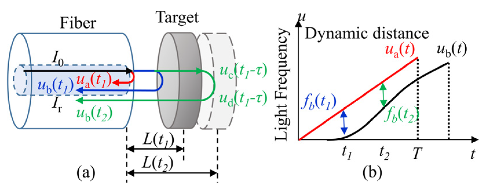
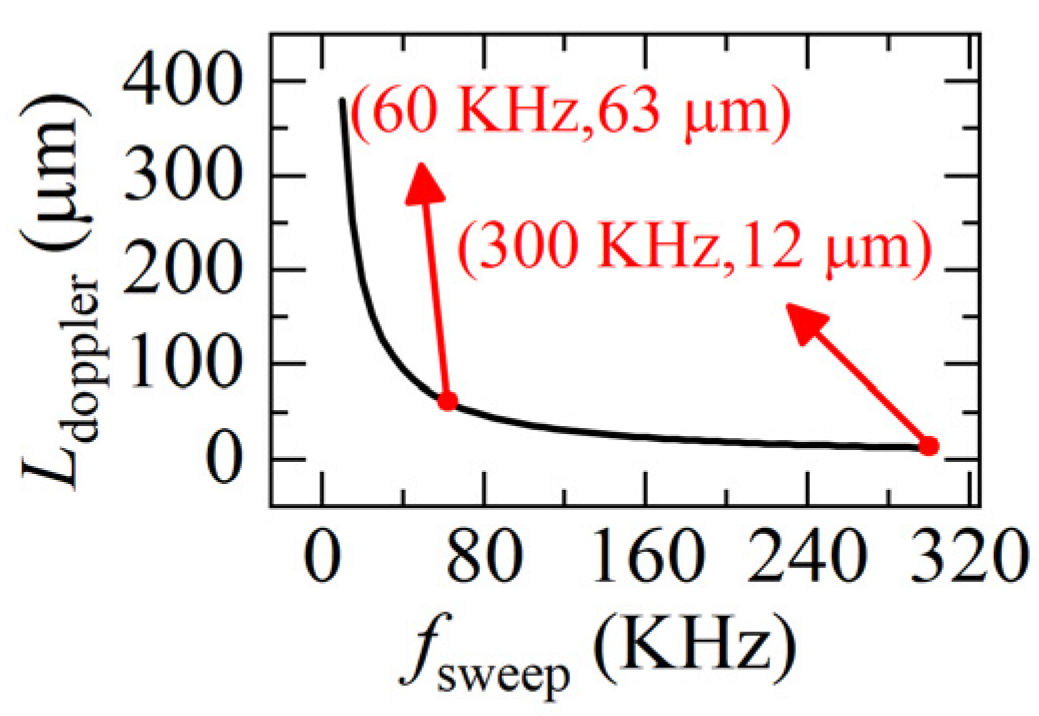
2. Principle of Reducing the Doppler-Induced Error

Figure 1a shows the schematic of a static distance measurement with an FSI system. One part of the light beam is reflected at the end face of the fiber, its frequency is recorded as u_a(t). The rest of light is transmitted out of the fiber and reflected by the target, then coupled back into the fiber, its frequency is recorded as u_b(t). The beat frequency can be written as [12]:

$$\begin{array}{ccc}\hfill f_b& =& u_a\left(t\right)-u_b\left(t\right)=\frac{\Delta u}{T}\cdot \frac{2n{L}_{sta}}{c}, 0\le t\le T\hfill \\ \hfill u\left(t\right)& =& u\left(0\right)+\frac{\Delta u}{T}t\hfill \end{array}$$

(1)

where n is the refractive index between the fiber end-face and the target, n = 1 when in the air; u is the optical frequency; Δu is the optical frequency range; c is the speed of light; f_b is the beat frequency of the FSI signal; t is the sweeping time; and T is the sweeping cycle.

Specifically, the light frequency u_a(t) and u_b(t) vary linearly in a sweeping cycle and the time delay between two beams is constant, as shown in Figure 1b. So, the beat frequency f_b is a constant in a sweeping cycle. According to Equation (1), the static distance is:

$$L_{sta}=\frac{cT}{2\Delta u}{f}_b$$

(2)

However, for a dynamic target shown in Figure 2, the distance L changes during a sweeping cycle, so the beat frequency f_b is no longer a constant. To analysis the instantaneous beat frequency, the light frequency reflected at fiber end-face is still assumed as u_a(t), the light frequency arriving at the target is u_c(t), the light travelling time from the fiber end-face to the target is τ, then, u_c(t) can be written as:

$$\begin{array}{ll}\hfill u_c\left(t\right)& =u_a\left(t-\tau \right),0\le t\le T\\ \hfill \tau & =\frac{L\left(t\right)}{c}\end{array}$$

(3)

Consider the Doppler effect, the light frequency reflected at the target u_d(t) is [13]:

$$u_d\left(t\right)=u_c\left(t\right)\frac{c-v\left(t\right)}{c+v\left(t\right)}\approx u_c\left(t\right)\left[1-\frac{2v\left(t\right)}{c}\right],0\le t\le T$$

(4)

where v(t) is the velocity of the target.

Assume that the light traveling time from the fiber end-face to the target is equal to the time from the target to the fiber end-face, the light frequency going back to the fiber end-face u_b(t) is:

$$u_b\left(t\right)=u_d\left(t-\tau \right),0\le t\le T$$

(5)

Then the instantaneous beat frequency is:

$$\begin{array}{ll}{f}_{bd}\left(t\right)& =u_a\left(t\right)-u_b\left(t\right)=u_a\left(t\right)-u_a\left(t-2\tau \right)\left[1-\frac{2v\left(t-2\tau \right)}{c}\right]\\ & \approx u_a\left(t\right)\frac{2v\left(t\right)}{c}+2\frac{\Delta u}{T}\tau ,0\le t\le T\end{array}$$

(6)

According to Equation (2), the dynamic instantaneous distance in a sweeping cycle is calculated to be:

$$\begin{array}{ll}{L}_{dyn}\left(t\right)& =\frac{cT}{2\Delta u}\left[u_a\left(t\right)\frac{2v\left(t\right)}{c}+2\frac{\Delta u}{T}\tau \right]=L\left(t\right)+u_a\left(t\right)\frac{T}{\Delta u}v\left(t\right)\\ & =L\left(t\right)+\frac{u_a\left(t\right)}{\Delta u\cdot f_{sweep}}v\left(t\right)=L+L_{doppler},0\le t\le T\end{array}$$

(7)

where f_sweep = 1/T, f_sweep is the sweeping rate.

The first term in Equation (7) is the real distance L, the second term is the Doppler-induced error L_error. We can see, L_error is related to the velocity of the target v(t) and the sweeping rate of the light f_sweep. As f_sweep increases, L_error rapidly decreases and then tends to be constant. When v(t) and light frequency are fixed, the greater the f_sweep is, the smaller the L_doppler is, as shown in Figure 3.

Although increasing the sweeping rate helps to reduce the Doppler-induced error L_doppler, it is still 12 μm at a very high sweeping rate (300 KHz), which is too large when compared to the distance variation of 0.3 μm.

The real instantaneous distance, which is the first term in Equation (7), can be further described to be [2]:

$$L\left(t\right)=L\left(0\right)+{\displaystyle {\int }_0^{t}v\left(t\right)}dt=L\left(0\right)+v\left(0\right)t+\frac{1}{2}a{t}^2,0\le t\le T$$

(8)

where L(0) is the initial distance in one sweeping cycle and a is the acceleration.

From Equation (7), we can see that when the sweeping cycle becomes small, the distance change in one sweeping cycle will also be small. At this time, take Equation (8) into Equation (7), let L_dyn(T), which is the distance at the end moment T of a sweeping cycle, represent the distance after the whole sweeping cycle. It is:

$$\begin{array}{ll}{L}_{dyn}\left(T\right)& =L\left(0\right)+v\left(0\right)T+\frac{1}{2}a{T}^2+\left(v\left(0\right)+aT\right)\frac{T{u}_a\left(T\right)}{\Delta u}\\ & =L\left(0\right)+v\left(0\right)T\left(1+\frac{u_a\left(T\right)}{\Delta u}\right)+\left(\frac{1}{2}+\frac{u_a\left(T\right)}{\Delta u}\right)a{T}^2\end{array}$$

(9)

In Equation (9), the sweeping cycle T is assumed to be sufficiently small. In this case, the distance change in one cycle is considered to be very small, the velocity or acceleration is regarded as a constant.

Define a Doppler coefficient to be:

$$A_{doppler}=1+\frac{u_a\left(T\right)}{\Delta u}$$

(10)

Let both sides of Equation (9) be divided by Equation (10) after moving L(0) in Equation (9) from right to the left. The distance variation is:

$$\Delta L_{mear}\left(T\right)=\frac{L_{dyn}\left(T\right)-L\left(0\right)}{A_{doppler}}=v\left(0\right)T+\frac{\Delta u+2u_a\left(T\right)}{2\left(\Delta u+u_a\left(T\right)\right)}a{T}^2$$

(11)

Then after further suppressing the Doppler-induced error, the measured distance is:

$$\begin{array}{ll}{L}_{mear}\left(T\right)& =L\left(0\right)+\Delta L_{mear}\left(T\right)=L\left(0\right)+v\left(0\right)T+\frac{\Delta u+2u_a\left(T\right)}{2\left(\Delta u+u_a\left(T\right)\right)}a{T}^2\\ & =L\left(0\right)+v\left(0\right)\frac{1}{f_{sweep}}+\frac{\Delta u+2u_a\left(T\right)}{2\left(\Delta u+u_a\left(T\right)\right)}\cdot \frac{a}{f_{sweep}^2}\end{array}$$

(12)

The principle residual error is expressed as:

$$L_{error}\left(T\right)=L\left(T\right)-L_{mear}\left(T\right)=\frac{u_a\left(T\right)}{2\left(\Delta u+u_a\left(T\right)\right)}a{T}^2=\frac{u_a\left(T\right)}{2\left(\Delta u+u_a\left(T\right)\right)}\cdot \frac{a}{f_{sweep}^2}$$

(13)

From Equation (13) we can see that L_error is related to a and T. When T is getting smaller, which means the sweeping rate f_sweep is higher, L_error decreases. The larger a is, the larger L_error becomes. Further simulation based on Equation (13) is given in Figure 4. When f_sweep is 60 KHz, the residual error L_error has been reduced to 0.13 nm and L_error is only 1.3 nm even when the acceleration a is 10 m/s². That is, we can suppress the Doppler-induced error to the order of a nanometer, by increasing the sweeping rate of the light frequency to some extent.

3. Demodulation of Dynamic Distance

3.1. Applicable Conditions of Frequency Demodulation

For a static distance measurement, the interference signal in one sweeping cycle is [14]:

$$s_{sta}\left(t\right)=\cos \left(2\pi f_{b}t+{\phi }_0\right),0\le t\le T$$

(14)

It is a standard cosine function with a single beat frequency f_b, as shown in Figure 5a. The fast Fourier transformation (FFT) can be used to get its interference frequency in the frequency domain shown in Figure 5b, then calculate the distance according to the relationship between beat frequency and distance using Equation (2).

For a dynamic target, the interference signal can be derived by the instantaneous beat frequency f_bd in Equation (6) as:

$$s_{dyn}(t)=\cos \left\{2\pi {\displaystyle {\int }_0^t{f}_{bd}}dt+{\phi }_0\right\}=\cos \left\{2\pi {\displaystyle {\int }_0^t\left[u_a(t)\frac{2v(t)}{c}+\frac{\Delta u}{T}\cdot \frac{2L(t)}{c}\right]}dt+{\phi }_0\right\},0\le t\le T$$

(15)

Equation (15) indicates that the beat frequency f_bd varies as the sweeping time t. The interference signal is not a uniform distribution, as shown in Figure 5a. To understand the signal from the frequency domain, the instantaneous beat frequency f_bd is obtained after applying the FFT to Equation (15), as shown in Figure 6. When f_sweep is low, the FFT spectrum contains multiple instantaneous frequencies (black curve), which correspond to the instantaneous distance change because of the movement of the target in a sweeping cycle. When f_sweep is gradually rising, the frequencies gradually merge (red curve).

When the ratio of f_sweep to the movement frequency of the target reaches “a certain value”, the frequencies merge into one peak (blue curve). That means, there is only one beat frequency, which is the same as the static distance situation (shown in Figure 5b). It can be considered that the movement of the target compared to the light frequency sweeping is quasi-static. Therefore, the FFT frequency algorithm, instead of the complex demodulation methods [15,16,17,18], can be used to demodulate the beat frequency then calculate the distance at the end moment of one sweeping cycle using Equation (12).

To analyze the quantitative condition of the quasi-static state, define ρ as the quasi-stationary coefficient to describe the ratio of the static beat frequency to the dynamic beat frequency, which is:

$$\rho =\frac{f_b}{f_{bd}}=\frac{2\frac{\Delta u}{T}\cdot \frac{L(t)}{c}}{\left(u_a(0)+\frac{\Delta u}{T}\cdot t\right)\cdot \frac{2v(t)}{c}+2\frac{\Delta u}{T}\cdot \frac{L(t)}{c}}\approx \frac{\Delta uL(T)}{u_a(T)v(T)\cdot \frac{1}{f_{sweep}}+\Delta uL(T)},(t\approx T)$$

(16)

Equation (16) shows that ρ is related to v(t) and f_sweep. Suppose v(t) is a cosine function to imitate the target moving at an arbitrary speed. That is:

$$v=\frac{dL}{dt}=2\pi \omega \cdot A\cos \left(2\pi \omega t\right),0\le t\le T$$

(17)

where A is the range of distance change and ω is the frequency.

The value ρ is simulated according to Equations (16) and (17), and plotted in Figure 7. The value of ρ is related to ω, A and f_sweep, as shown in Figure 7a. To understand the relationship between ρ and f_sweep more clearly, extract some specific curves when A is ±10 μm, ±50 μm, and ±100 μm and plot in Figure 7b–d. It shows that, as the sweeping rate f_sweep of the laser increases, ρ gradually approaches a constant, which indicates the movement of the target compared to the light frequency-sweeping is quasi-static. However, the quasi-static state is affected by ω and A. Comparing the f_sweep corresponding to the points with ρ = 0.9 and ω = 1000 Hz in Figure 7b–d, it can be seen that ρ rises slower when A is larger. That is, the larger the ω or A, the longer ρ takes to reach a constant, the larger the corresponding f_sweep. Therefore, before using the FFT frequency algorithm, the highest frequency ω_max and the range of distance change A need to be calculated. For a simple calculation, when f_sweep is around 20~50 times larger than the highest frequency of distance, the FFT algorithm would work, according to Figure 7 and is demonstrated by our practice.

3.2. Demodulation Algorithm

The FSI signal is actually a discrete sampled signal. The sampling points are equal to the swept points of the light frequency. To increase the resolution of FFT, a zero-padding extension to the discrete signal is often applied. Then, according to the FFT algorithm:

$$S\left[k\right]={\displaystyle \sum _{n=0}^{N_{FFT}-1}{s}_{dyn}\left[n\right]}{e}^{-i\frac{2\pi }{N_{FFT}}nk}.$$

(18)

where s[n] is the discrete form of Equation (15), N_FFT is the length of s[n] after applying the zero-padding extension.

The distance is calculated to be:

$$L_{FFT}=\frac{cT}{2\Delta u}\cdot \frac{n_{\max }}{N_{FFT}}$$

(19)

where n_max is the location of the peak frequency.

The demodulated distance L_corr contains the real distance L and the Doppler-induced error L_doppler. According to Equations (11) and (12), the measured distance L_mear after suppressing the Doppler-induced error is:

$$L_{mear}=\frac{L_{FFT}-L\left(0\right)}{A_{doppler}}+L\left(0\right)$$

(20)

The data processing flow is shown in Figure 8. The first process of the raw spectrum is the mean value removing, normalization and zero-padding extension. Then, the distance is obtained using the FFT algorithm. After the Doppler-induced error compensation according to Equation (20), the dynamic distance can be demodulated.

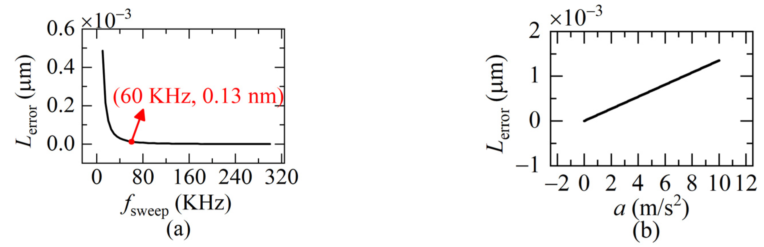
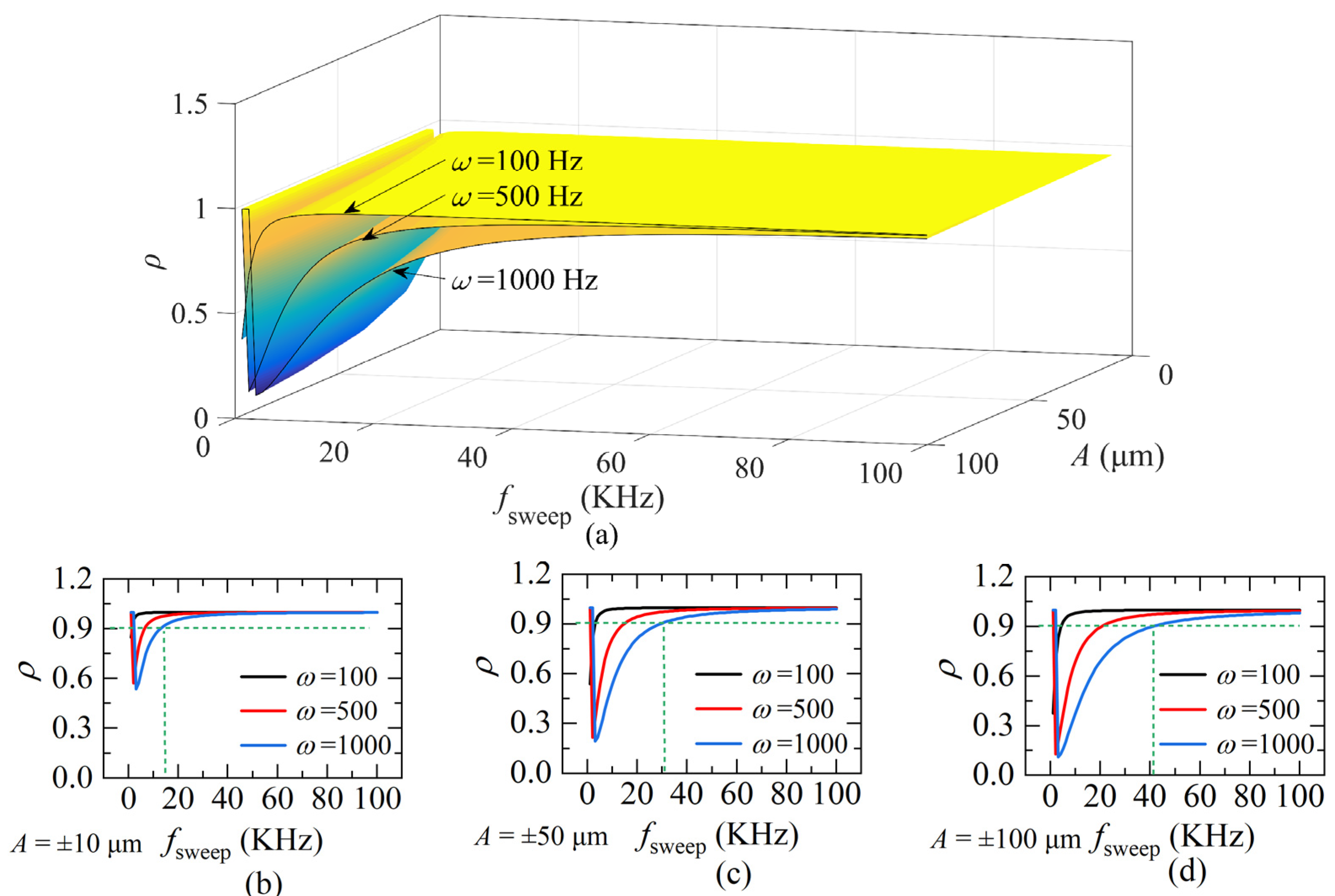
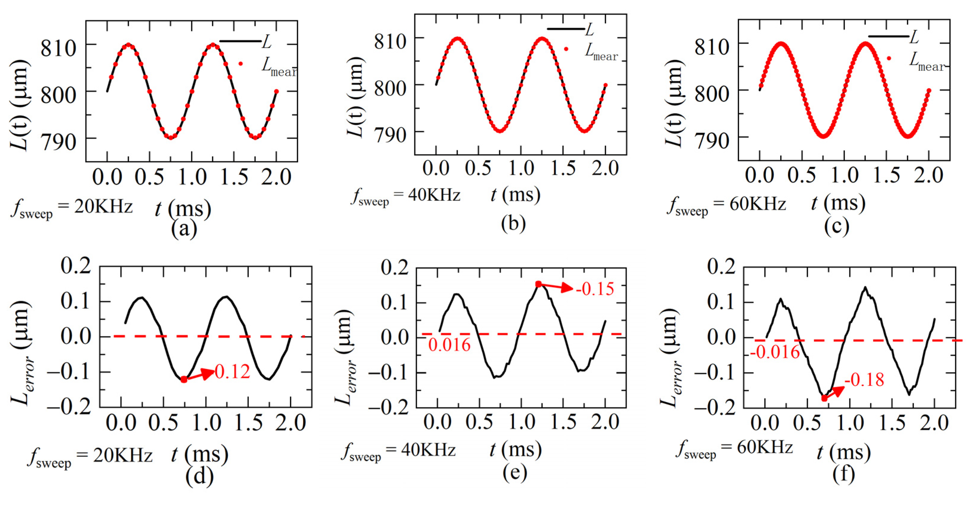
3.3. Simulation

In order to verify the analysis above, a dynamic distance L(t) varies as a sinusoidal function which is given as:

$$L\left(t\right)=L\left(0\right)+A\sin (2\pi \omega \cdot t),0\le t\le T$$

(21)

Figure 9a shows the distance L(t) varies as a sinusoidal function according to Equation (21). When the sweeping cycle T = 0.05 ms and the sweeping rate f_sweep = 1/T = 20 KHz, the variation of the distance in one sweeping cycle is shown as Figure 9b, which is corresponding to the red part in Figure 9a.

According to the quasi-static state condition, when the frequency of the dynamic distance is 1 KHz, the sweeping rates of the laser f_sweep is set 20 KHz, 40 KHz or 60 KHz. The demodulation results are calculated by our proposed method and shown in Figure 10a–c, respectively. The corresponding demodulation errors for each sweeping rate are shown in Figure 10d–f. The mean value of the absolute demodulation error is 0–0.019 μm and the maximum value is 0.13–0.16 μm, accounting for 0.3% of the demodulation range (60 μm). Results show our proposed method is able to achieve high demodulation accuracy even when the dynamic distance is in the form of a sinusoidal function, which means both velocity and acceleration are changing during sweeping.

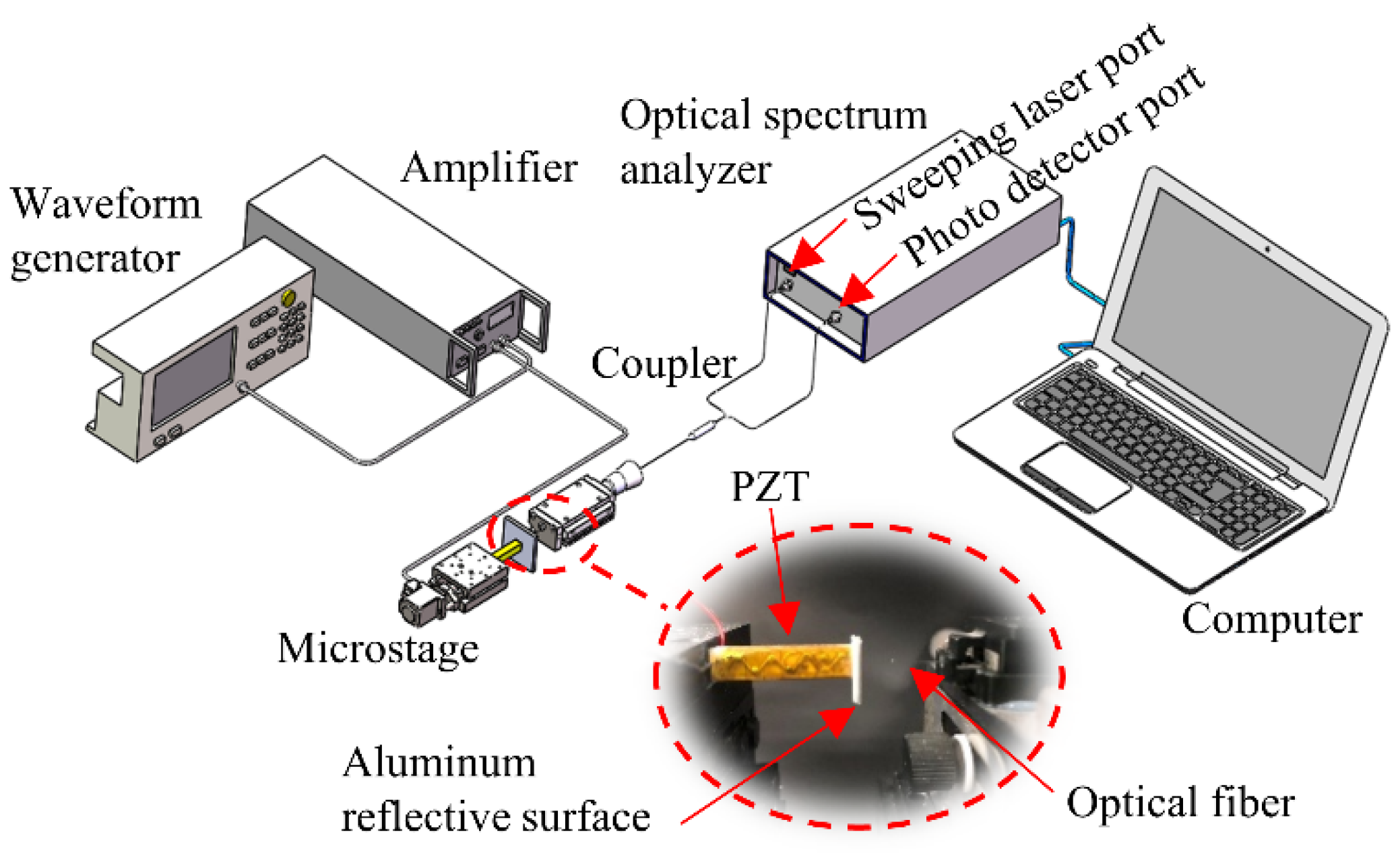
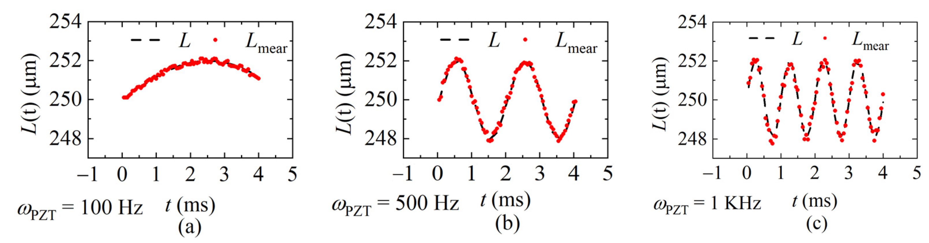
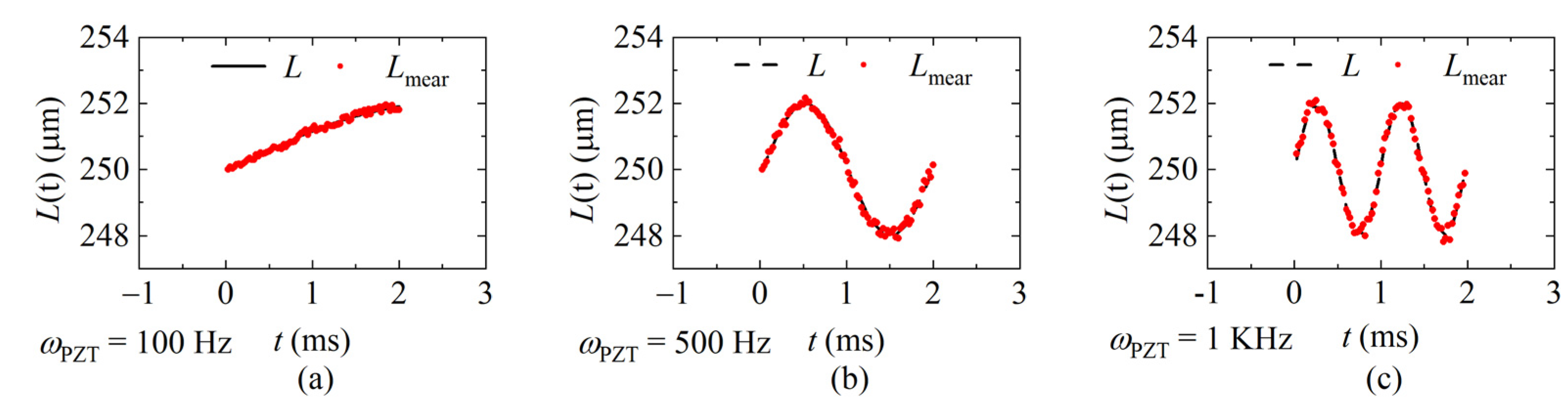
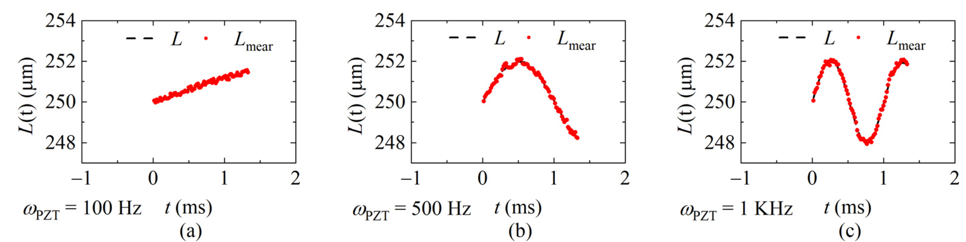
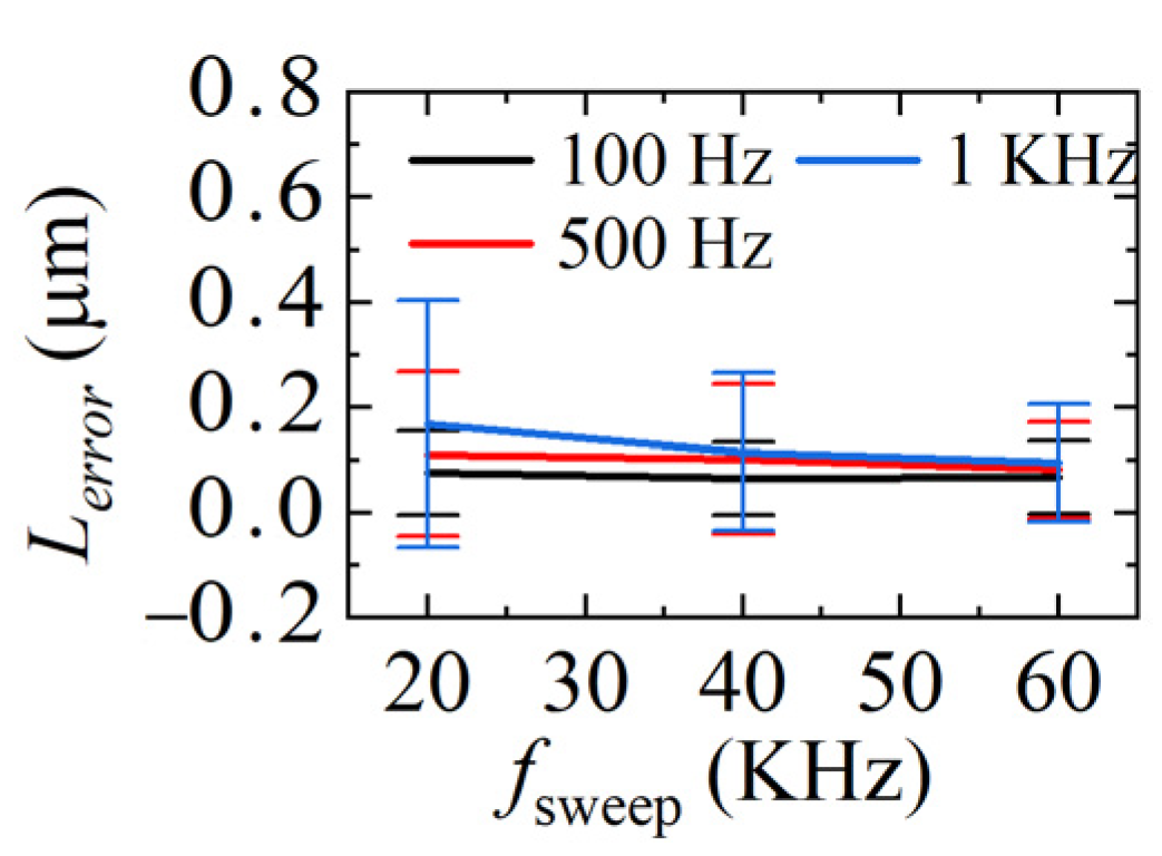
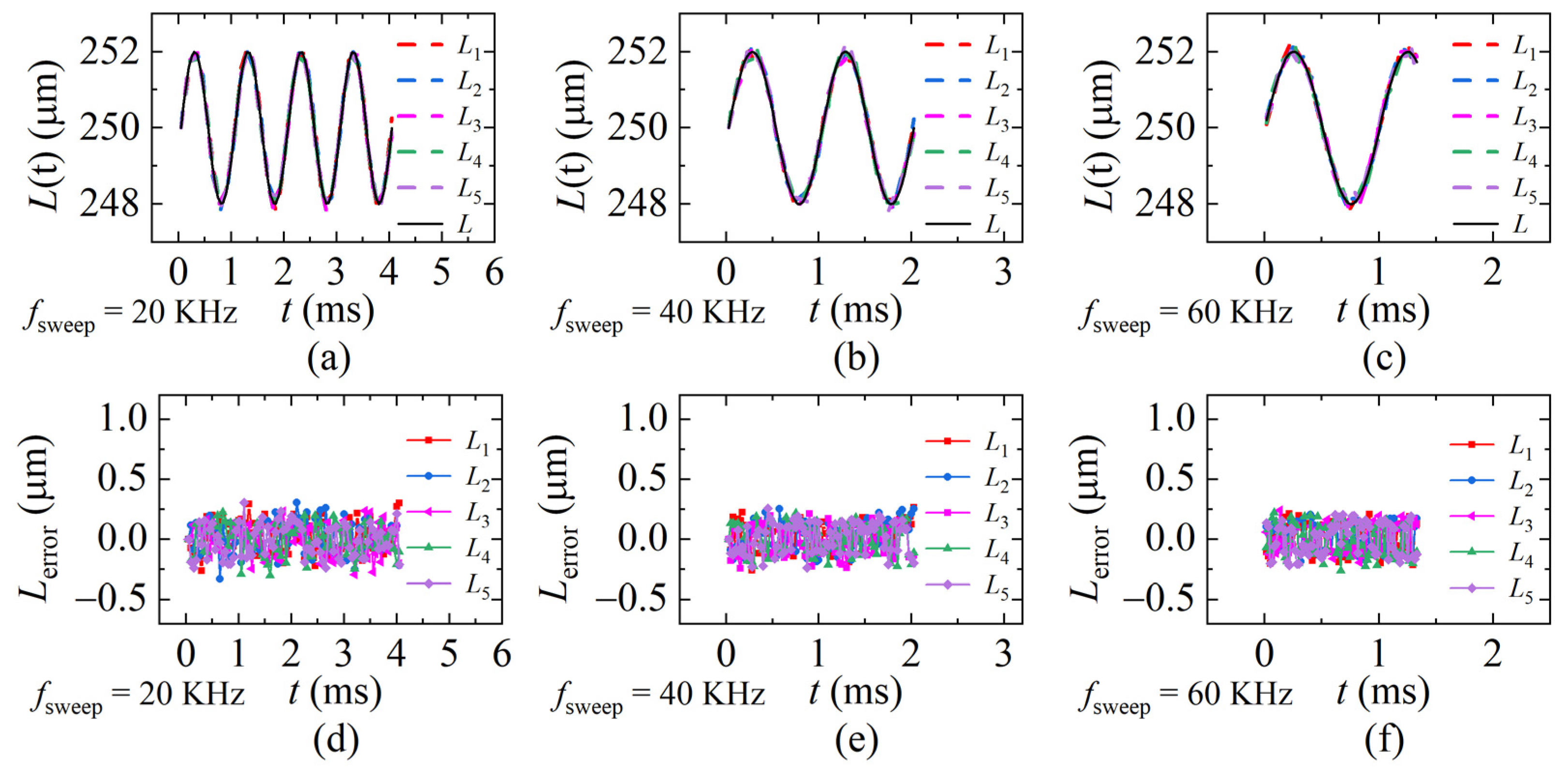
4. Experiment

The dynamic distance measurement experiment was carried out to verify the proposed method, as shown in Figure 11. The distance was formed by the gap between the fiber end-face and the PZT (Pk4FA2H3P2, Thorlabs, Newton, NJ, USA). The PZT was driven by a signal generator (DG4102, RIGOL) and the amplifier (Has 4011, NF Corporation, Yokohama, Japan). The optical fiber was connected to a frequency-swept laser (Arcadia Optronix, Zhuhai, China, GC-760001c-01) and the photodetector module (Xilinx Artix-7, Conquer, Beijing, China). The entire setup was placed on a vibration-isolated optical stage.

The sinusoidal vibration frequency of the PZT was set to 100 Hz, 500 Hz, and 1 KHz, and the laser was scanned at different frequency intervals. The dynamic distance was expressed as:

$$L=L\left(0\right)+A_{PZT}\sin (2\pi {\omega }_{PZT}\times t)$$

(22)

where L(0) is 250 μm, ω_PZT is the PZT vibration frequency, and the vibration amplitude A_PZT = ±2 μm.

The interference spectra of each sweeping cycle were collected by the laser at the sweeping rates of 20 KHz, 40 KHz, and 60 KHz, respectively, and the demodulation results were calculated according to the data processing flow shown in Figure 8 and given in Figure 12, Figure 13 and Figure 14. Figure 12 shows the demodulation distances with f_sweep = 20 KHz, and the frequency of the distance is ω_PZT of 100 Hz, 500 Hz, and 1 KHz, respectively. Figure 13 shows f_sweep = 40 KHz and Figure 14 shows f_sweep = 60 KHz. The red dots indicate the demodulated distance, and the black delineated lines are the ideal distance according to the parameters of the signal generator.

The demodulation errors between the demodulated distances and ideal distances in Figure 12, Figure 13 and Figure 14 are calculated and given in Figure 15. The average standard deviation is 0.14 μm, 0.11 μm, and 0.09 μm when f_sweep is 20 KHz, 40 KHz, and 60 KHz, respectively. The larger f_sweep, the smaller the fluctuation of the demodulated distance, which means the smaller the error, the mean value of the demodulation errors in each condition is plotted in Figure 16. It can be seen that when f_sweep is fixed, L_error increases with the increase in the ω_PZT; when ω_PZT is fixed, L_error decreases with the increase in f_sweep. The maximum error is 0.41 μm and the minimum error is 0.001 μm.

To verify the repeatability of the proposed method, five identical dynamic experiments were conducted when f_sweep is 20 KHz, 40 KHz, and 60 KHz. The PZT vibration-frequency ω_PZT is 1 KHz in the repeatability experiments. The demodulation results were calculated and are shown in Figure 17a–c. Corresponding errors are shown in Figure 17d–f. The average standard deviation of each sweeping rate is 0.133 μm, 0.122 μm, and 0.123 μm. It can be seen from the comparison that the larger f_sweep is, the smaller the error is when ω_PZT is a constant.

5. Conclusions

A Doppler-induced error compensation model based on a scheme to increase the frequency sweeping rate is proposed. A distance demodulation method combining a Fourier transformation and a correlation-like algorithm is investigated when the defined quasi-stationary coefficient approaches a constant. Simulations and experiments based on dynamic distance with a sinusoidal change demonstrate that the proposed method has a standard deviation of 0.09 μm within a distance range of 4 μm at a sweeping rate of 60 KHz.

The proposed method is based only on the basic FSI system without any additional devices which can greatly simplify the hardware system; it is also based on the FFT and correlation-like algorithm instead of complex methods, which can simplify the calculation.

References

- Hartmann, L.; Meiners-Hagen, K.; Abou-Zeid, A. An absolute distance interferometer with two external cavity diode lasers. Meas. Sci. Technol. 2008, 19, 045307–045313. [Google Scholar] [CrossRef]
- Tao, L.; Liu, Z.; Zhang, W.; Zhou, Y. Frequency-scanning interferometry for dynamic absolute distance measurement using Kalman filter. Opt. Lett. 2014, 39, 6997–7000. [Google Scholar] [CrossRef]
- Zhang, F.; Li, Y.; Pan, H.; Shi, C.; Qu, X. Vibration Compensation of the Frequency-Scanning-Interferometry-Based Absolute Ranging System. Appl. Sci. 2019, 9, 147. [Google Scholar] [CrossRef] [Green Version]
- Schneider, R.; Thurmel, P.; Stockman, M. Distance measurement of moving objects by frequency modulated laser radar. Opt. Eng. 2001, 40, 33–37. [Google Scholar] [CrossRef]
- Dale, J.; Hughes, B.; Lancaster, A.J.; Lewis, A.J.; Reichold, A.J.H.; Warden, M.S. Multi-channel absolute distance measurement system with sub ppm-accuracy and 20 m range using frequency scanning interferometry and gas absorption cells. Opt. Express 2014, 22, 24869–24893. [Google Scholar] [CrossRef]
- Warden, M.S. Absolute Distance Metrology Using Frequency Swept Lasers. Ph.D. Thesis, Oxford University, Oxford, UK, 2011. [Google Scholar]
- Prellinger, G.; Meiners-Hagen, K.; Pollinger, F. Spectroscopicallyin situtraceable heterodyne frequency-scanning interferometry for distances up to 50 m. Meas. Sci. Technol. 2015, 26, 084003. [Google Scholar] [CrossRef]
- Lu, C.; Xiang, Y.; Gan, Y.; Liu, B.; Chen, F.; Liu, X.; Liu, G. FSI-based non-cooperative target absolute distance measurement method using PLL correction for the influence of a nonlinear clock. Opt. Lett. 2018, 43, 2098–2101. [Google Scholar] [CrossRef]
- Shao, B.; Zhang, W.; Zhang, P.; Chen, W. Dynamic Clearance Measurement Using Fiber-Optic Frequency-Swept and Frequency-Fixed Interferometry. IEEE Photon. Technol. Lett. 2020, 32, 1331–1334. [Google Scholar] [CrossRef]
- Swinkels, B.L.; Bhattacharya, N.; Braat, J.J.M. Correcting movement errors in frequency-sweeping interferometry. Opt. Lett. 2005, 30, 2242–2244. [Google Scholar] [CrossRef] [Green Version]
- Jia, X.; Liu, Z.; Tao, L.; Deng, Z. Frequency-scanning interferometry using a time-varying Kalman filter for dynamic tracking measurements. Opt. Express 2017, 25, 25782–25796. [Google Scholar] [CrossRef] [PubMed]
- Moro, E.A.; Todd, M.D.; Puckett, A.D. Understanding the effects of Doppler phenomena in white light Fabry–Perot interferometers for simultaneous position and velocity measurement. Appl. Opt. 2012, 51, 6518–6527. [Google Scholar] [CrossRef] [PubMed]
- Gjurchinovski, A. The Doppler effect from a uniformly moving mirror. Eur. J. Phys. 2005, 26, 643–646. [Google Scholar] [CrossRef]
- Chen, X.; Wang, X.; Pan, S. Accuracy enhanced distance measurement system using double-sideband modulated frequency scanning. Opt. Eng. 2017, 56, 036114–036119. [Google Scholar] [CrossRef]
- Shang, Y.; Lin, J.; Yang, L.; Liu, Y.; Wu, T.; Zhou, Q.; Zhu, J. Precision improvement in frequency scanning interferometry based on suppression of the magnification effect. Opt. Express 2020, 28, 5822–5834. [Google Scholar] [CrossRef] [PubMed]
- Kakuma, S.; Katase, Y. Frequency Scanning Interferometry Immune to Length Drift Using a Pair of Vertical-Cavity Surface-Emitting Laser Diodes. Opt. Rev. 2012, 9, 376–380. [Google Scholar] [CrossRef]
- Jia, X.; Liu, Z.; Deng, Z.; Deng, W.; Wang, Z.; Zhen, Z. Dynamic absolute distance measurement by frequency sweeping interferometry based Doppler beat frequency tracking model. Opt. Commun. 2019, 430, 163–169. [Google Scholar] [CrossRef]
- Deng, Z.; Liu, Z.; Jia, X.; Deng, W.; Zhang, X. Dynamic cascade-model-based frequency-scanning interferometry for real-time and rapid absolute optical ranging. Opt. Express 2019, 27, 21929–21945. [Google Scholar] [CrossRef] [PubMed]
Publisher’s Note: MDPI stays neutral with regard to jurisdictional claims in published maps and institutional affiliations. |
© 2022 by the authors. Licensee MDPI, Basel, Switzerland. This article is an open access article distributed under the terms and conditions of the Creative Commons Attribution (CC BY) license (https://creativecommons.org/licenses/by/4.0/).
Share and Cite
Chen, Y.; Lei, X.; Xiao, L.; Zhang, P.; Liu, X. Dynamic Distance Measurement Based on a Fast Frequency-Swept Interferometry. Sensors 2022, 22, 4771. https://doi.org/10.3390/s22134771
Chen Y, Lei X, Xiao L, Zhang P, Liu X. Dynamic Distance Measurement Based on a Fast Frequency-Swept Interferometry. Sensors. 2022; 22(13):4771. https://doi.org/10.3390/s22134771
Chicago/Turabian StyleChen, Yuru, Xiaohua Lei, Lin Xiao, Peng Zhang, and Xianming Liu. 2022. "Dynamic Distance Measurement Based on a Fast Frequency-Swept Interferometry" Sensors 22, no. 13: 4771. https://doi.org/10.3390/s22134771