
Estimation of Greenhouse Lettuce Growth Indices Based on a Two-Stage CNN Using RGB-D Images


Abstract
:1. Introduction
2. Materials and Methods
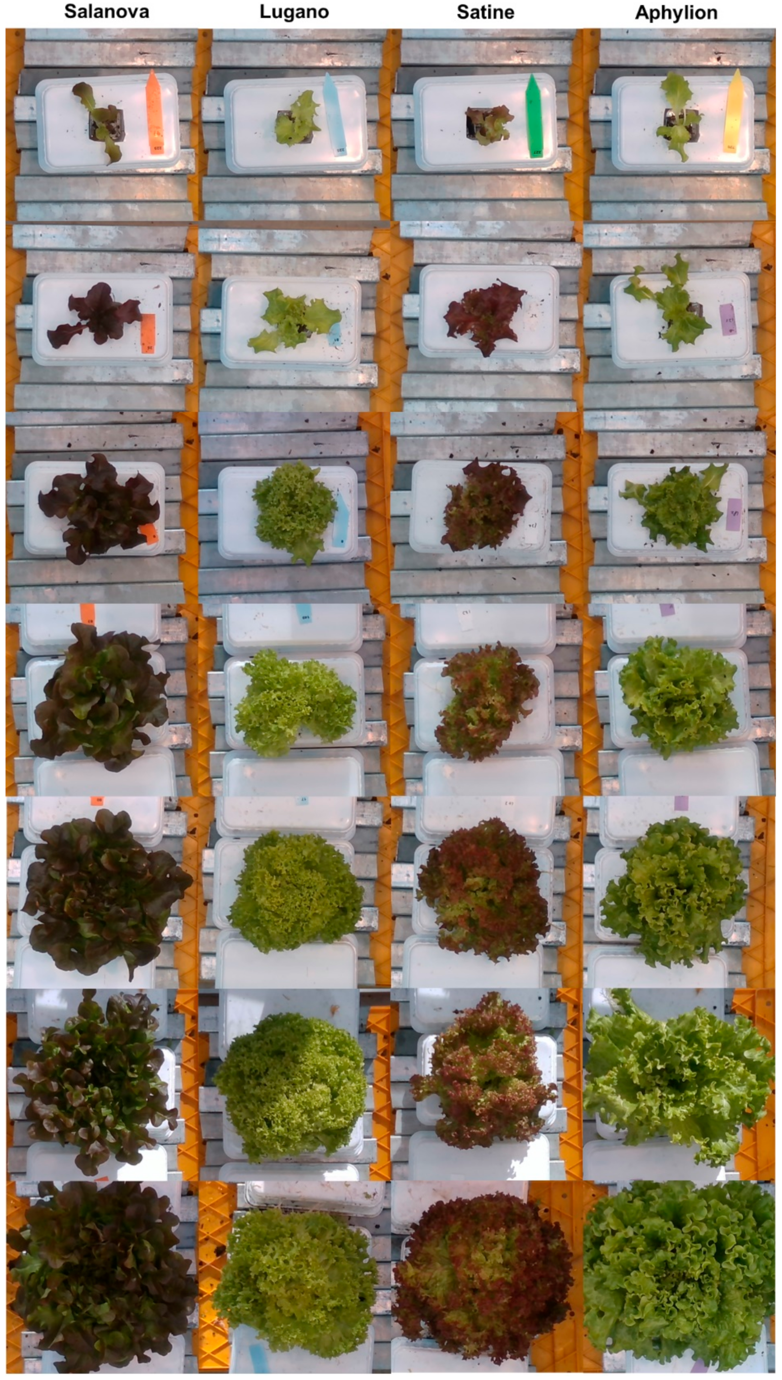
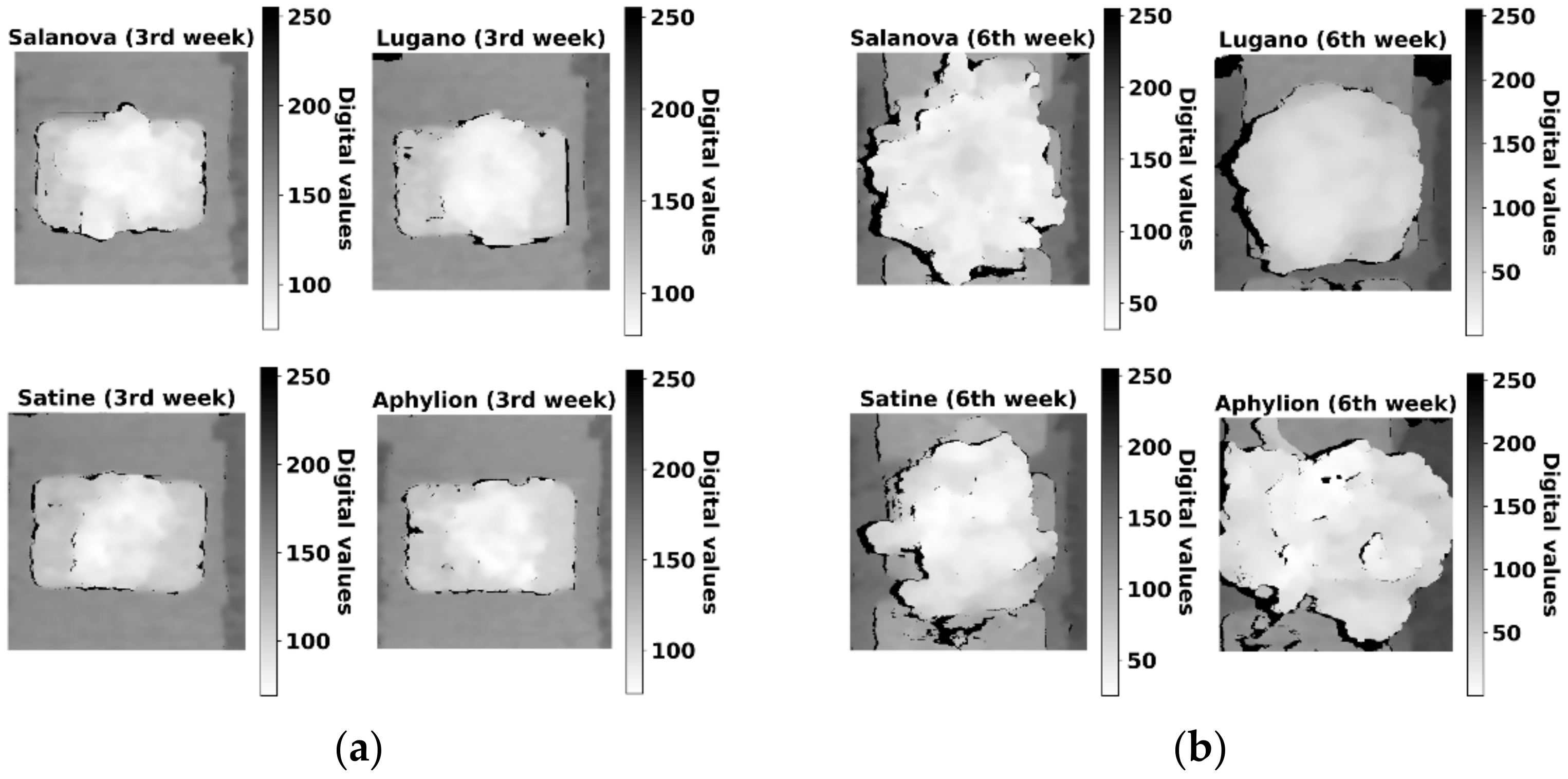
2.1. Dataset
2.2. Image Preprocessing
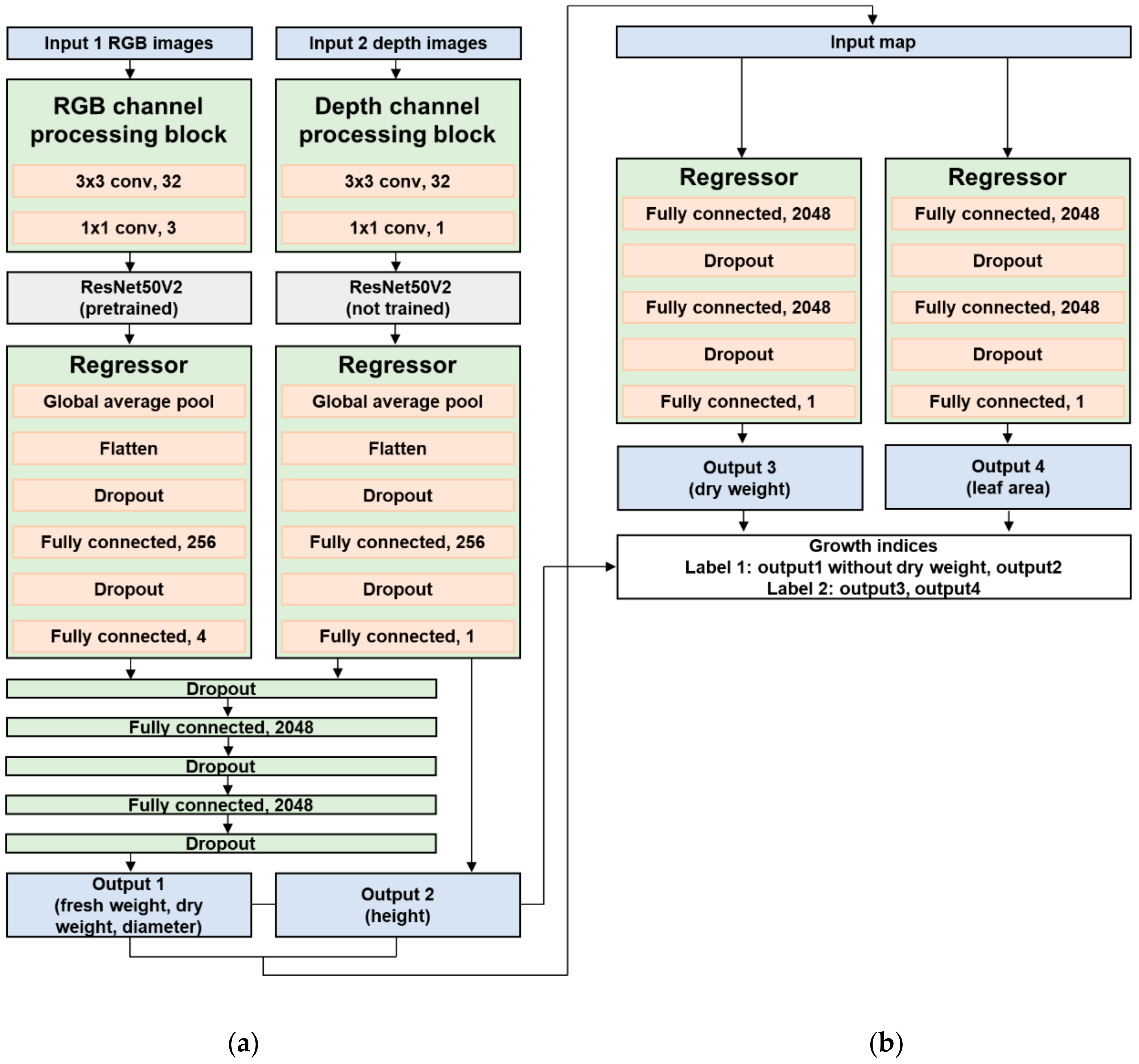
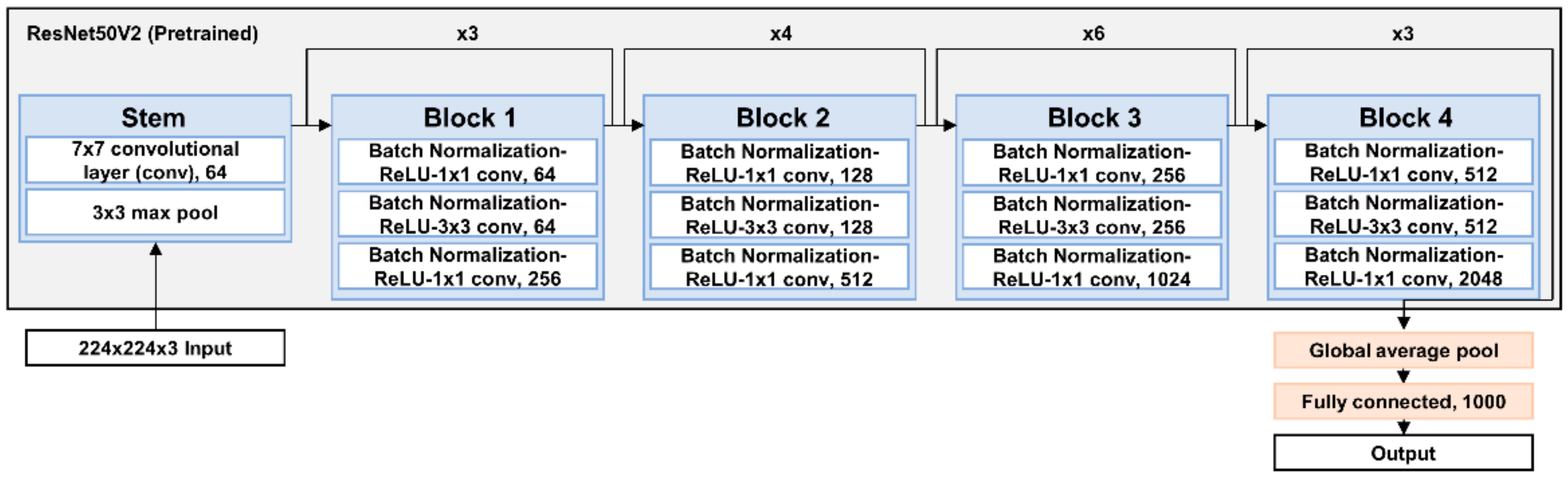
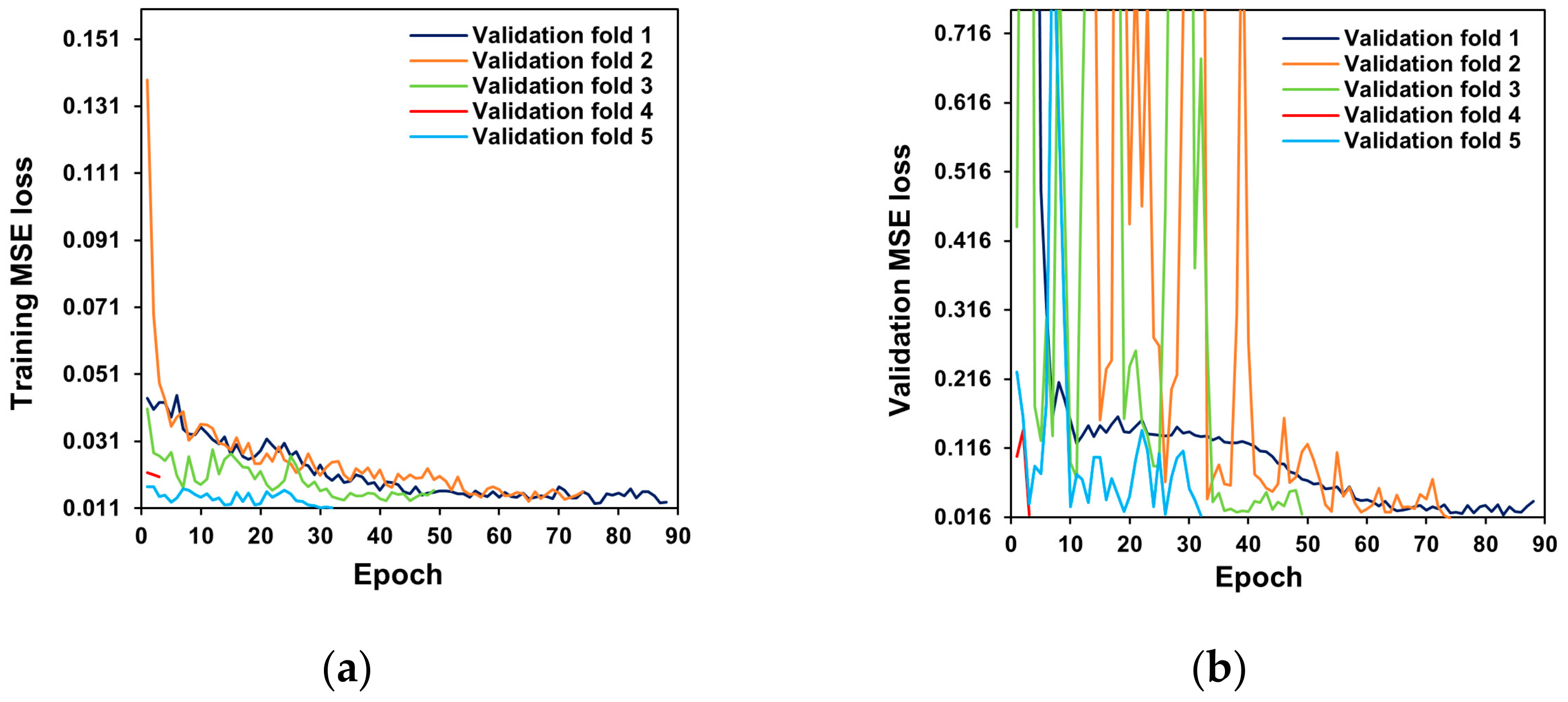
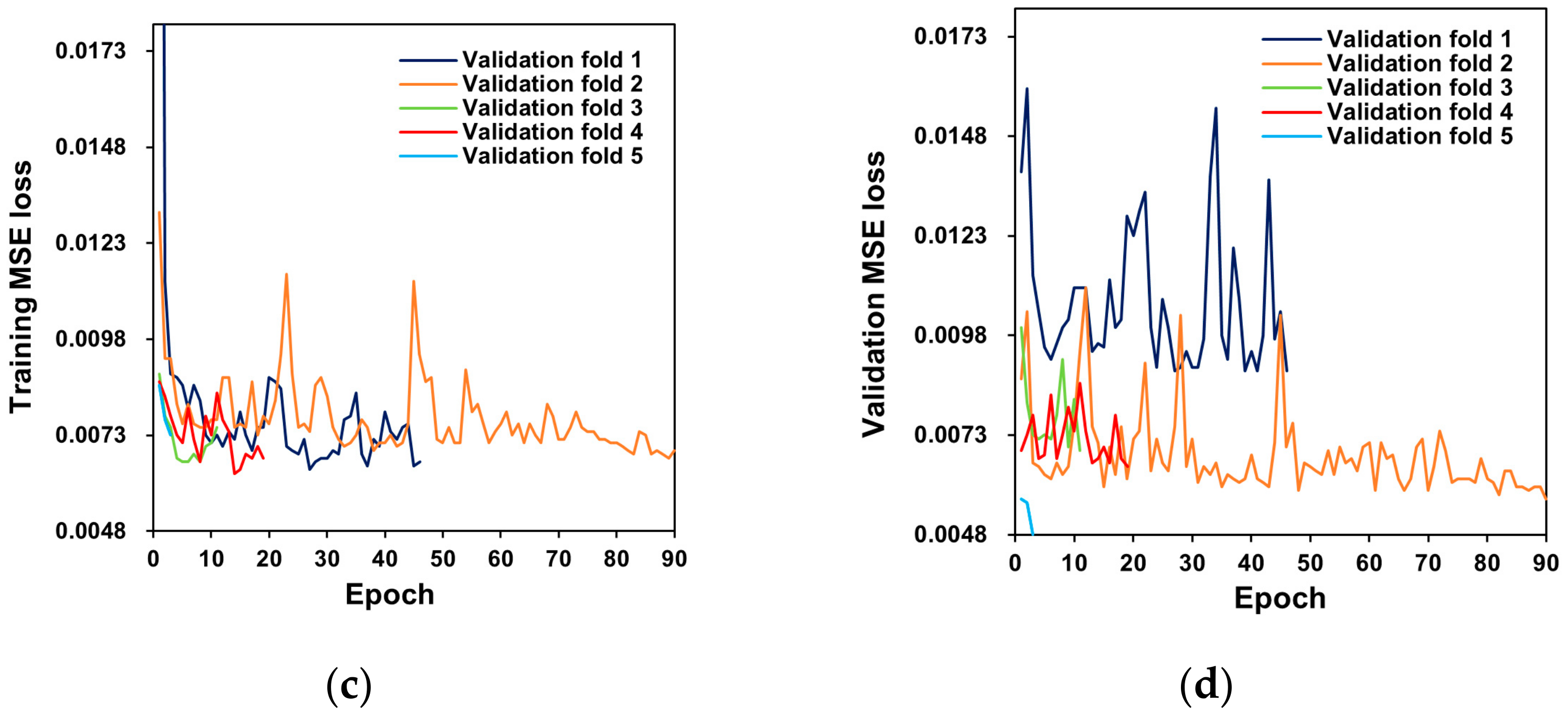
2.3. Network Architecture and Training
2.4. Model Evaluation
3. Results and Discussion
4. Conclusions
Author Contributions
Funding
Institutional Review Board Statement
Informed Consent Statement
Data Availability Statement
Conflicts of Interest
References
- Smart, R.E. Principles of grapevine canopy microclimate manipulation with implications for yield and quality: A review. Am. J. Enol. Vitic. 1985, 36, 230–239. [Google Scholar]
- Williams, L.E. Growth of ‘Thompson Seedless’ grapevines. I. Leaf area development and dry weight distribution. J. Am. Soc. Hortic. Sci. 1987, 112, 325–330. [Google Scholar]
- Allen, R.G.; Pereira, L.S.; Raes, D.; Smith, M. Crop Evapotranspiration-Guidelines for Computing Crop Water Requirements-FAO Irrigation and Drainage Paper 56; Food and Agriculture Organization of the United Nations: Rome, Italy, 1998. [Google Scholar]
- Pearcy, R.W.; Ehleringer, J.R.; Mooney, H.; Rundel, P.W. Plant Physiological Ecology: Field Methods and Instrumentation; Springer Science & Business Media: Berlin, Germany, 2021. [Google Scholar]
- Cho, Y.Y.; Oh, S.; Oh, M.M.; Son, J.E. Estimation of individual leaf area, fresh weight, and dry weight of hydroponically grown cucumbers (Cucumis sativus L.) using leaf length, width, and SPAD value. Sci. Hortic. 2007, 111, 330–334. [Google Scholar] [CrossRef]
- Peksen, E. Non-destructive leaf area estimation model for faba bean (Vicia faba L.). Sci. Hortic. 2007, 113, 322–328. [Google Scholar] [CrossRef]
- Lati, R.N.; Filin, S.; Eizenberg, H. Plant growth parameter estimation from sparse 3D reconstruction based on highly-textured feature points. Precis. Agric. 2013, 14, 586–605. [Google Scholar] [CrossRef]
- Yeh, Y.-H.F.; Lai, T.-C.; Liu, T.-Y.; Liu, C.-C.; Chung, W.-C.; Lin, T.-T. An automated growth measurement system for leafy vegetables. Biosyst. Eng. 2014, 117, 43–50. [Google Scholar] [CrossRef]
- Jiang, J.S.; Kim, H.J.; Cho, W.J. On-the-go image processing system for spatial mapping of lettuce fresh weight in plant factory. IFAC-PapersOnLine 2018, 51, 130–134. [Google Scholar] [CrossRef]
- Jin, X.; Zarco-Tejada, P.J.; Schmidhalter, U.; Reynolds, M.P.; Hawkesford, M.J.; Varshney, R.K.; Yang, T.; Nie, C.; Li, Z.; Ming, B.; et al. High-throughput estimation of crop traits: A review of ground and aerial phenotyping platforms. IEEE Trans. Geosci. Remote Sens. 2021, 9, 200–231. [Google Scholar] [CrossRef]
- Sze, V.; Chen, Y.H.; Yang, T.J.; Emer, J.S. Efficient processing of deep neural networks: A tutorial and survey. Proc. Inst. Electr. Electron. Eng. 2017, 105, 2295–2329. [Google Scholar] [CrossRef] [Green Version]
- Dyrmann, M.; Karstoft, H.; Midtiby, H.S. Plant species classification using deep convolutional neural network. Biosyst. Eng. 2016, 151, 72–80. [Google Scholar] [CrossRef]
- Hasan, A.M.; Sohel, F.; Diepeveen, D.; Laga, H.; Jones, M.G. A survey of deep learning techniques for weed detection from images. Comput. Electron. Agric. 2021, 184, 106067. [Google Scholar] [CrossRef]
- Jiang, Y.; Li, C. Convolutional neural networks for image-based high-throughput plant phenotyping: A review. Plant Phenomics 2020, 2020, 4152816. [Google Scholar] [CrossRef] [Green Version]
- Fu, L.; Gao, F.; Wu, J.; Li, R.; Karkee, M.; Zhang, Q. Application of consumer RGB-D cameras for fruit detection and localization in field: A critical review. Comput. Electron. Agric. 2020, 177, 105687. [Google Scholar] [CrossRef]
- Liu, J.; Wang, X. Plant diseases and pests detection based on deep learning: A review. Plant Methods 2021, 17, 22. [Google Scholar] [CrossRef]
- Vasanthi, V. Crop growth monitoring and leaf area index estimation using wireless sensor network and CNN. In Proceedings of the 2021 Third International Conference on Inventive Research in Computing Applications (ICIRCA), Coimbatore, India, 2–4 September 2021. [Google Scholar] [CrossRef]
- Jin, S.; Su, Y.; Song, S.; Xu, K.; Hu, T.; Yang, Q.; Guo, Q. Non-destructive estimation of field maize biomass using terrestrial lidar: An evaluation from plot level to individual leaf level. Plant Methods 2020, 16, 69. [Google Scholar] [CrossRef]
- Liu, W.; Li, Y.; Liu, J.; Jiang, J. Estimation of plant height and aboveground biomass of Toona sinensis under drought stress using RGB-D imaging. Forests 2021, 12, 1747. [Google Scholar] [CrossRef]
- Lu, J.Y.; Chang, C.L.; Kuo, Y.F. Monitoring growth rate of lettuce using deep convolutional neural networks. In Proceedings of the 2019 ASABE Annual International Meeting, Boston, MA, USA, 7–10 July 2019. [Google Scholar] [CrossRef]
- Reyes-Yanes, A.; Martinez, P.; Ahmad, R. Real-time growth rate and fresh weight estimation for little gem romaine lettuce in aquaponic grow beds. Comput. Electron. Agric. 2020, 179, 105827. [Google Scholar] [CrossRef]
- Zhang, L.; Xu, Z.; Xu, D.; Ma, J.; Chen, Y.; Fu, Z. Growth monitoring of greenhouse lettuce based on a convolutional neural network. Hortic. Res. 2020, 7, 124. [Google Scholar] [CrossRef]
- Mortensen, A.K.; Bender, A.; Whelan, B.; Barbour, M.M.; Sukkarieh, S.; Karstoft, H.; Gislum, R. Segmentation of lettuce in coloured 3D point clouds for fresh weight estimation. Comput. Electron. Agric. 2018, 154, 373–381. [Google Scholar] [CrossRef]
- Jiang, Y.; Li, C.; Paterson, A.H.; Sun, S.; Xu, R.; Robertson, J. Quantitative analysis of cotton canopy size in field conditions using a consumer-grade RGB-D camera. Front. Plant Sci. 2018, 8, 2233. [Google Scholar] [CrossRef] [Green Version]
- Yan, G.; Hu, R.; Luo, J.; Weiss, M.; Jiang, H.; Mu, X.; Zhang, W. Review of indirect optical measurements of leaf area index: Recent advances, challenges, and perspectives. Agric. For. Meteorol. 2019, 265, 390–411. [Google Scholar] [CrossRef]
- Kolhar, S.; Jagtap, J. Plant trait estimation and classification studies in plant phenotyping using machine vision–A review. Inf. Process. Agric. 2021. [Google Scholar] [CrossRef]
- Quan, L.; Li, H.; Li, H.; Jiang, W.; Lou, Z.; Chen, L. Two-stream dense feature fusion network based on RGB-D data for the real-time prediction of weed aboveground fresh weight in a field environment. Remote Sens. 2021, 13, 2288. [Google Scholar] [CrossRef]
- Raja, P.V.; Olenskyj, A.; Kamangir, H.; Earles, M. Simultaneously predicting multiple plant traits from multiple sensors using deformable CNN regression. In Proceedings of the 2022 AI for Agriculture and Food Systems (AIAFS), Vancouver, BC, Canada, 28 February–1 March 2022. [Google Scholar] [CrossRef]
- Li, J.; Wang, M. An end-to-end deep RNN based network structure to precisely regress the height of lettuce by single perspective sparse point cloud. In Proceedings of the 2022 North American Plant Phenotyping Network (NAPPN), Athens, GA, USA, 22–25 February 2022. [Google Scholar] [CrossRef]
- Hemming, S.; de Zwart, H.F.; Elings, A.; Bijlaard, M.; van Marrewijk, B.; Petropoulou, A. 3rd Autonomous Greenhouse Challenge: Online Challenge Lettuce Images. Available online: https://doi.org/10.4121/15023088.v1 (accessed on 2 March 2022).
- Chang, A.; Jung, J.; Maeda, M.M.; Landivar, J. Crop height monitoring with digital imagery from unmanned aerial system (UAS). Comput. Electron. Agric. 2017, 141, 232–237. [Google Scholar] [CrossRef]
- Olaniyi, J.O.; Akanbi, W.B.; Adejumo, T.A.; Ak, O.G. Growth, fruit yield and nutritional quality of tomato varieties. Afr. J. Food Sci. 2010, 4, 398–402. [Google Scholar]
- Evans, G.C. The Quantitative Analysis of Plant Growth; University of California Press: Berkeley, CA, USA, 1972; Volume 1. [Google Scholar]
- Maimaitijiang, M.; Sagan, V.; Sidike, P.; Hartling, S.; Esposito, F.; Fritschi, F.B. Soybean yield prediction from UAV using multimodal data fusion and deep learning. Remote Sens. Environ. 2020, 237, 111599. [Google Scholar] [CrossRef]
- Ahmed, A.K.; Cresswell, G.C.; Haigh, A.M. Comparison of sub-irrigation and overhead irrigation of tomato and lettuce seedlings. J. Hortic. Sci. Biotechnol. 2000, 75, 350–354. [Google Scholar] [CrossRef]
- Kaselimi, M.; Protopapadakis, E.; Voulodimos, A.; Doulamis, N.; Doulamis, A. Multi-channel recurrent convolutional neural networks for energy disaggregation. IEEE Access 2019, 7, 81047–81056. [Google Scholar] [CrossRef]
- Bacchi, S.; Zerner, T.; Oakden-Rayner, L.; Kleinig, T.; Patel, S.; Jannes, J. Deep learning in the prediction of ischaemic stroke thrombolysis functional outcomes: A pilot study. Acad. Radiol. 2020, 27, e19–e23. [Google Scholar] [CrossRef] [PubMed]
- Zang, H.; Liu, L.; Sun, L.; Cheng, L.; Wei, Z.; Sun, G. Short-term global horizontal irradiance forecasting based on a hybrid CNN-LSTM model with spatiotemporal correlations. Renew. Energ. 2020, 160, 26–41. [Google Scholar] [CrossRef]
- Yang, H.; Wang, L.; Huang, C.; Luo, X. 3D-CNN-Based sky image feature extraction for short-term global horizontal irradiance forecasting. Water 2021, 13, 1773. [Google Scholar] [CrossRef]
- Fix, E.; Hodges, J.L. Discriminatory analysis. Nonparametric discrimination: Consistency properties. Int. Stat. Rev. 1989, 57, 238–247. [Google Scholar] [CrossRef]
- Goodfellow, I.; Bengio, Y.; Courville, A. Deep Learning; MIT Press: Cambridge, MA, USA, 2016. [Google Scholar]
- Deng, J.; Dong, W.; Socher, R.; Li, L.J.; Li, K.; Fei-Fei, L. ImageNet: A large-scale hierarchical image database. In Proceedings of the 2009 IEEE Conference on Computer Vision and Pattern Recognition, Miami, FL, USA, 20–25 June 2009. [Google Scholar] [CrossRef] [Green Version]
- He, K.; Zhang, X.; Ren, S.; Sun, J. Identity mappings in deep residual networks. In Proceedings of the European Conference on Computer Vision, Amsterdam, The Netherlands, 8–16 October 2016. [Google Scholar] [CrossRef] [Green Version]
- He, K.; Zhang, X.; Ren, S.; Sun, J. Deep residual learning for image recognition. In Proceedings of the 2016 IEEE Conference on Computer Vision and Pattern Recognition, Las Vegas, NV, USA, 27–30 June 2016. [Google Scholar] [CrossRef] [Green Version]
- Kingma, D.P.; Ba, J. Adam: A Method for Stochastic Optimization. arXiv 2015, arXiv:1412.6980. Available online: https://arxiv.org/abs/1412.6980 (accessed on 2 March 2022).
- Nair, V.; Hinton, G.E. Rectified linear units improve restricted Boltzmann machines. In Proceedings of the 27th International Conference on Machine Learning, Haifa, Israel, 21–24 June 2010. [Google Scholar]
- Mosteller, F.; Tukey, J.W. Data Analysis, Including Statistics; Addison-Wesley: Boston, MA, USA, 1968; pp. 80–203. [Google Scholar]
- Golzarian, M.R.; Frick, R.A.; Rajendran, K.; Berger, B.; Roy, S.; Tester, M.; Lun, D.S. Accurate inference of shoot biomass from high-throughput images of cereal plants. Plant Methods 2011, 7, 2. [Google Scholar] [CrossRef] [Green Version]
- Feng, H.; Jiang, N.; Huang, C.; Fang, W.; Yang, W.; Chen, G.; Liu, Q. A hyperspectral imaging system for an accurate prediction of the above-ground biomass of individual rice plants. Rev. Sci. Instrum. 2013, 84, 095107. [Google Scholar] [CrossRef]
- Rice, L.; Wong, E.; Kolter, Z. Overfitting in adversarially robust deep learning. In Proceedings of the 37th International Conference on Machine Learning, Vienna, Autria, 13–18 July 2020. [Google Scholar]
- Ying, X. An overview of overfitting and its solutions. In Proceedings of the 2018 International Conference on Computer Information Science and Application Technology, Daqing, China, 7–9 December 2018. [Google Scholar]


| Week | RGB-Image (Salanova) | Fresh Weight (g) | Dry Weight (g) | Height (cm) | Diameter (cm) | Leaf Area (cm2) |
|---|---|---|---|---|---|---|
| 1 |  | 5.2 | 0.58 | 9.8 | 17.2 | 202.7 |
| 2 |  | 16.4 | 1.22 | 6.8 | 18.5 | 520.1 |
| 3 |  | 69.8 | 4.16 | 9.0 | 25.1 | 1694.3 |
| 4 |  | 85.0 | 5.02 | 8.0 | 25.0 | 2008.8 |
| 5 |  | 110.0 | 6.04 | 12.0 | 28.0 | 2414.7 |
| 6 |  | 133.2 | 6.84 | 15.8 | 32.0 | 3089.2 |
| 7 |  | 236.5 | 11.04 | 17.0 | 33.5 | 5348.1 |
| Fresh Weight (g) | Dry Weight (g) | Height (cm) | Diameter (cm) | Leaf Area (cm2) | |
|---|---|---|---|---|---|
| Minimum | 1.4 | 0.09 | 4.3 | 8.2 | 57.6 |
| Maximum | 459.7 | 20.1 | 25 | 37 | 5868 |
| Fresh Weight (g) | Dry Weight (g) | Height (cm) | Diameter (cm) | Leaf Area (cm2) | |
|---|---|---|---|---|---|
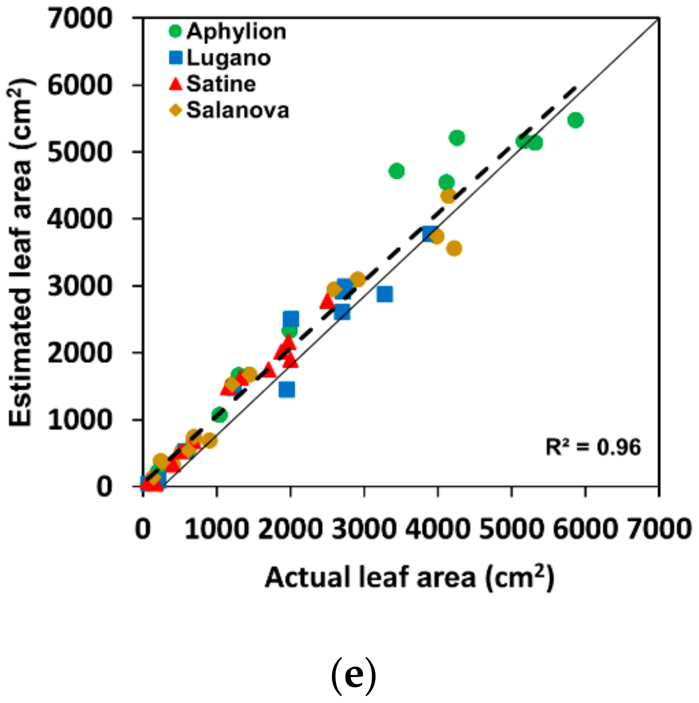
| R2 | 0.95 | 0.95 | 0.95 | 0.89 | 0.96 |
| RMSE 1 | 27.85 | 1.26 | 1.53 | 2.28 | 326.04 |
| NRMSE 2 (%) | 6.09 | 6.30 | 7.65 | 7.92 | 5.62 |
| Fresh Weight (R2) | Dry Weight (R2) | Height (R2) | Diameter (R2) | Leaf Area (R2) | |
|---|---|---|---|---|---|
| Aphylion | 0.96 | 0.96 | 0.96 | 0.92 | 0.96 |
| Lugano | 0.93 | 0.91 | 0.91 | 0.86 | 0.96 |
| Satine | 0.96 | 0.99 | 0.95 | 0.92 | 0.98 |
| Salanova | 0.95 | 0.95 | 0.91 | 0.96 | 0.97 |
| Total | 0.95 | 0.95 | 0.95 | 0.89 | 0.96 |
| Loading Time per Image (s) | Loading Time per 50 Images (s) | Inference Time per Image (s) | Inference Time per 50 Images (s) | |
|---|---|---|---|---|
| i7-11700 and RTX-3090 PC | 0.03 ± 0.001 | 0.52 ± 0.015 | 0.13 ± 0.044 | 0.55 ± 0.079 |
| Jetson SUB mini-PC | 0.034 ± 0.004 | 2.56 ± 0.990 | 0.49 ± 0.190 | 5.59 ± 0.108 |
Publisher’s Note: MDPI stays neutral with regard to jurisdictional claims in published maps and institutional affiliations. |
© 2022 by the authors. Licensee MDPI, Basel, Switzerland. This article is an open access article distributed under the terms and conditions of the Creative Commons Attribution (CC BY) license (https://creativecommons.org/licenses/by/4.0/).
Share and Cite
Gang, M.-S.; Kim, H.-J.; Kim, D.-W. Estimation of Greenhouse Lettuce Growth Indices Based on a Two-Stage CNN Using RGB-D Images. Sensors 2022, 22, 5499. https://doi.org/10.3390/s22155499
Gang M-S, Kim H-J, Kim D-W. Estimation of Greenhouse Lettuce Growth Indices Based on a Two-Stage CNN Using RGB-D Images. Sensors. 2022; 22(15):5499. https://doi.org/10.3390/s22155499
Chicago/Turabian StyleGang, Min-Seok, Hak-Jin Kim, and Dong-Wook Kim. 2022. "Estimation of Greenhouse Lettuce Growth Indices Based on a Two-Stage CNN Using RGB-D Images" Sensors 22, no. 15: 5499. https://doi.org/10.3390/s22155499
APA StyleGang, M.-S., Kim, H.-J., & Kim, D.-W. (2022). Estimation of Greenhouse Lettuce Growth Indices Based on a Two-Stage CNN Using RGB-D Images. Sensors, 22(15), 5499. https://doi.org/10.3390/s22155499