Abstract
Accurate indoor location information has considerable social and economic value in applications, such as pedestrian heatmapping and indoor navigation. Ultrasonic-based approaches have received significant attention mainly since they have advantages in terms of positioning with temporal correlation. However, it is a great challenge to gain accurate indoor localization due to complex indoor environments such as non-uniform indoor facilities. To address this problem, we propose a fusion localization method in the indoor environment that integrates the localization information of inertial sensors and acoustic signals. Meanwhile, the threshold scheme is used to eliminate outliers during the positioning process. In this paper, the estimated location is fused by the adaptive distance weight for the time difference of arrival (TDOA) estimation and improved pedestrian dead reckoning (PDR) estimation. Three experimental scenes have been developed. The experimental results demonstrate that the proposed method has higher localization accuracy in determining the pedestrian location than the state-of-the-art methods. It resolves the problem of outliers in indoor acoustic signal localization and cumulative errors in inertial sensors. The proposed method achieves better performance in the trade-off between localization accuracy and low cost.
1. Introduction
Location-based services (LBS) emerged under the promotion of technical development and social demands and have become a very popular research topic in recent years. According to statistics, 80% of people’s activities are completed in an indoor environment. The demands of indoor localization for indoor navigation services, and material positioning have been growing and have great social and commercial value and broad application prospects.
Researchers have conducted a series of related works on indoor localization technologies (e.g., WIFI fingerprints [1], geomagnetic [2] and ultrasonic [3] techniques). Of all of these technologies, the ultrasonic-based localization method is calculated using geometric distance. It has high localization accuracy for low propagation speeds compared with radio signals. Furthermore, ultrasonic-based localization systems do not require the deployment of extra devices due to their compatibility with smartphones. Refs. [4,5] used a time difference of arrival (TDOA) measurement for ultrasonic and radio frequency signals to measure the distance between two locations. Afterward, the location estimation was calculated using the trilateral method. Although indoor localization based on acoustic signals can achieve high-precision localization, it still cannot solve the errors caused by the indoor environments and building structures. Different ambient sound signals need to be specifically set according to the environment. The heterogeneity of buildings still hinders the universal application of acoustic signal localization.
In indoor localization based on PDR, data are collected by inertial sensors, which are not affected by the surrounding environments. At present, all smartphones and tablets on the market have been installed with the integrated inertial measurement unit (IMU), which solves the hardware problem of using this technology for localization. Refs. [6,7] describes the autocorrelation analysis method for step detection, which has high accuracy but poor adaptability to motion changes. The zero crossing detection method was used for step detection in [8]; it is easy to implement, but not suitable for real-time research. In [9,10], the peak detection method was used for step detection, and it has less resource consumption and good real-time performance. This method has the advantages of low cost and high autonomy without extra infrastructures. However, accumulated localization errors over time cause low localization accuracy.
In summary, it is difficult to balance cost, accuracy, and stability. Ultrasonic waves are susceptible to the surrounding environment (mirror reflection, limited beam angle, walls, shadows, etc.), and anomalies occur in the TDOA estimation, which can lead to large localization errors. Due to inertia, cumulative errors in PDR estimation hinder extensive application in realistic scenes. Single-mode indoor localization limits the application scenes in the existing localization technologies. In this paper, a multimodal fusion localization algorithm is proposed. Using this method, the localization accuracy is improved and the pervasiveness of location application is enhanced in an indoor scene. However, there are two major challenges in realizing such a fusion localization system.
- How can one balance low cost and high localization? In the popularization of applications, we often hope to achieve low cost and high precision to meet the requirements of localization. However, high precision often requires high-cost infrastructures. Therefore, the trade-off between cost and accuracy is the key to indoor localization.
- How can one fuse the acoustic and inertia localization? Different localization results vary with different methods. The contribution of each localization result is not uniform in the localization process. Therefore, determining the importance of each method and fusing the multimodal method remains a challenge.
To address the above challenges, we propose an ultrasonic-based fusion localization system. The system can achieve higher precision indoor localization with low cost and retain the advantages of the acoustic signals and PDR localization while overcoming the effects of acoustic localization occlusion and the PDR cumulative error. The main contributions of this paper are as follows:
- An improved PDR method: Based on the compatibility of mobile phones with ultrasonic signals and inertial sensor positioning, a fusion localization method is proposed to solve the contradiction between cost and accuracy. To gain high location estimation, we propose an improved PDR method. The experimental results show that our method has better localization performance than the traditional PDR method. Afterward, we propose a threshold method to eliminate the anomalies, and the localization accuracy is improved.
- An adaptive weight based on the distance fusion scheme: To balance the contribution of the localization results, we propose an adaptive weight based on a distance scheme that estimates the weight value for acoustic and improved PDR localization. Based on the weight values, we fuse the acoustic estimation and improved inertial estimation to achieve accurate pedestrian location.
The organization of the rest of the paper is as follows: in Section 2, related work is presented, followed by the workflow of our localization system in Section 3. We introduce the indoor localization system with sound signals, PDR, and fused localization algorithms in Section 4. The illustrative experimental results are provided in Section 5. Section 6 summarizes the research results presented in this paper.
Notations shows the major symbols used in this article.
2. Related Works
Indoor localization has been extensively studied for decades. Scholars have adopted various signals to develop related works, including ultra-wideband (UWB) [11,12,13], WIFI [14,15,16], Radio Frequency Identification (RFID) [17,18], Bluetooth [19,20], Geomagnetic sequence [21,22] and Ultrasonic signals [3,23]. Despite the accuracy in special trial sites, they have a few practical limitations that hinder their wide deployment. UWB-based and RFID-based systems need to install special infrastructure, which has high costs. Infrared-based localization technology is often blocked by indoor building structures and has no pervasiveness due to complex indoor environments. WIFI signals, Bluetooth signals and geomagnetic sequences need to construct a fingerprint database beforehand and are updated from time to time to adapt to surrounding environment changes. More human resources are needed.
Localization based on ultrasonic signals has recently attracted much attention, mainly since it is compatible with mobile phones, deployable without infrastructure support, and has high localization accuracy. Therefore, researchers have begun to study indoor localization with ultrasonic signals. The typical localization system based on ultrasonic signals [24,25] uses the TDOA to estimate the pedestrian location. Shuangshuang Li [26] et al. proposed a TDOA-based localization algorithm for underwater acoustic sensor networks. In this network, the maximum likelihood (ML) ratio criterion was adopted to reduce acoustic localization errors. Ref. [27] presented an acoustic localization algorithm based on a decadal stereo array. Gergely Vakulya [28] et al. proposed an adaptive consistency-function-based solution localization algorithm for cooperative and consistent errors. Suresh Manickam [29] et al. proposed a multisource distributed localization algorithm. Hu et al. proposed a TDOA localization method based on improved the TPSN and KF [30], and it improved the accuracy due to time synchronization. Yu-Ting Wang et al. proposed a zero-configuration indoor localization solution using asynchronous acoustic beacons [31]. Based on the clock synchronization problem in the TDOA real-time localization system, Ge Yan et al. proposed a cross-check synchronization method [32] and the soft clock synchronization design of the TDOA positioning system on the DW1000 module. The method contains the communication protocol of the master base station with slave base stations and user tags and arranges the communication time slots between modules to solve the problem of mutual interference of communication signals. Liu [33] first proposed the positioning system GuoGuo using a smartphone as a positioning terminal and achieved a positioning accuracy of 6–25 cm using a pseudo-random code acoustic signal in the 15 kHz to 20 kHz frequency band. Patrick Lazik [34] et al. achieved a localization accuracy of 10 cm using chirp acoustic signals.
Inertial measurement technology does not rely on additional equipment for auxiliary localization. It can be located in all weather and terrain. Lei Cheng [35] et al. proposed a fusion method that adopted the Kalman filter to fuse binocular vision and an inertial navigation system (INS). Jishi Cui [36] et al. proposed an indoor localization system in which an improved Zee method and regularized particle filters were used to improve the cumulative error of the PDR algorithm. Rohan Kumar Yadav [37] et al. proposed an indoor localization method based on BLE beacons and IMUs to enhance accuracy.
Localization based on acoustic and inertial sensors has made remarkable achievements. However, environmental error is still not well eliminated. Therefore, the single acoustic localization method still cannot meet the practical requirements of cost and accuracy. Combining acoustic localization with IMU auxiliary localization is a good scheme for environmental effects, and this strategy not only achieves high accuracy but also has relatively low equipment cost. The multimodal fusion system that we propose adopts an adaptive distance weighting approach to estimate the location.
3. System Workflow
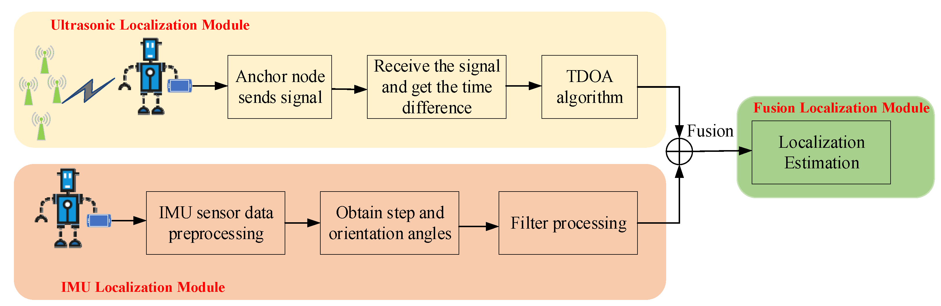
In this section, we overview the workflow of the fusion localization method in Figure 1, which includes three parts: the TDOA estimation-based ultrasonic signal, the estimation based IMU and the fusion localization estimation.
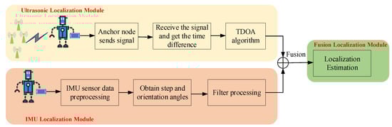
Figure 1.
Overall scheme of the fusion localization system.
In this workflow, the first stage involves the collection of ultrasonic and inertial sensor signals. The volunteer holds smartphone in the heading direction at constant speed. The ultrasonic and inertial sensor signals are collected automatically by the client applications installed on the smartphone, and sent to the server. In the server ultrasonic signals are extracted and preprocessed, and the TDOA estimation module determines the target location. In localization based on IMU, the acceleration, gyroscope, magnetometer and heading angles are extracted from the server and are preprocessed. According to the IMU data, we obtain the target location using the improved PDR method. Finally, accuracy localization estimation is achieved by fusing the TDOA estimation and IMU estimation.
4. Fusion Localization Based on Ultrasonic and Inertial Signals
We illustrate the design of the fusion localization method and provide an overview of the proposed fusion system in Section 4.1. Afterward, Section 4.2 illustrates data extraction and preprocessing. Section 4.3 introduces the estimation based on acoustic and IMU signals, and Section 4.4 illustrates the adaptive weight value generation. Finally, the fusion localization estimation is shown in Section 4.5.
4.1. Overview
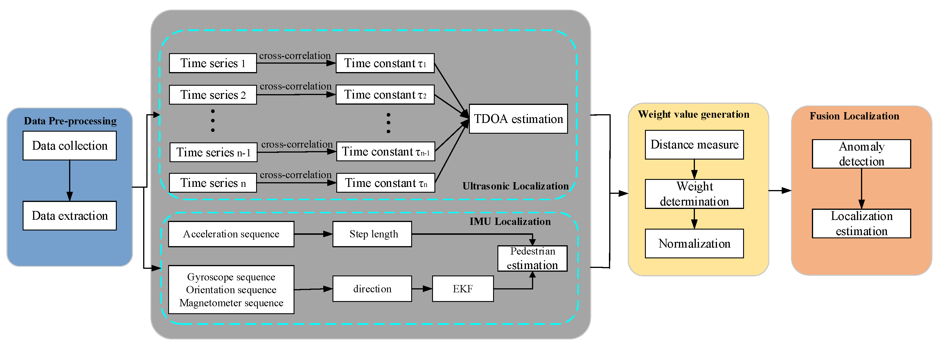
In this section, we introduce the multimodal fusion localization system. The detailed technical implementation structure is presented in Figure 2. First, we extract the ultrasonic signal, acceleration, magnetometer and gyroscope sequences from the client. Afterward, we adopt the TDOA algorithm to determine the target with ultrasonic signals. For the acceleration, magnetometer and gyroscope sequences, the improved PDR algorithm, which localizes the target, is presented. To identify the importance, we generate weight values for the two methods. Finally, we fuse the two locations with adaptive weight values to obtain the final location for the target.
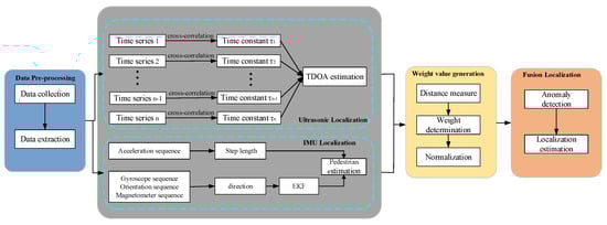
Figure 2.
Detailed technical implementation of the proposed fuse localization system.
More specifically, our system includes the following components:
Data extraction and preprocessing: In this part, we collect the data using the application installed on the smartphone and send data to servers. The ultrasonic signals and inertial data from the IMU are extracted from the received data.
Target coarse determination: In this module, the location of the target is perceived using ultrasonic signals and inertial data. The TDOA algorithm is adopted to calculate the target location with acoustic signals. For the inertial data, the improved PDR is presented to estimate the target.
Adaptive weight value generation: The different models in each location have different importance. After finishing the target coarse determination, we propose an adaptive weight value generation mechanism based on the localization of the current time and former time.
Fusion localization: Based on the weight value, we design a fusion localization estimation method for ultrasonic and inertial sequences.
4.2. Data Extraction and Preprocessing
A chirp signal is a widely used pulse compression signal, and it is a typical non-smooth signal with good autocorrelation characteristics. It can still be detected by correlation operations even with severe signal fading. In this paper, the chirp signal is used as the ultrasonic signal, which is defined as follows:
where is the initial frequency of the chirp signal, is the modulation rate, and is the duration time.
Signals with different frequency ranges have various transmission characteristics in indoor environments. To validate this assertion, we sample the acoustic signal with an in vivo Y85a smartphone, in which the frequency range is 0−25 kHz, and the acoustic source is HUAWEI Nova 4 devices. Figure 3 shows the spectrum of the received signals at the trial site. The spectrums of acoustic signals are relatively stable below 15 kHz and the range of 17−20 kHz, and a sharp drop between 15 kHz and 17 kHz. Therefore, considering the requirements of indoor localization, we choose chirp signals with a frequency range of 17−19 kHz.
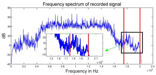
Figure 3.
Spectrum analysis of in vivo Y85a transmit and MEIZU 16 s Pro receive signals.
We deployed multiple acoustic anchors with a pair of microphones and speakers at fixed locations. The microphone and speaker at the anchor point are spatially separated. Each anchor message consists of a preamble, an identifier (id), a sequence number (seqno.) and local timestamp (ts). The anchor node decodes the message from the anchors including itself. The target devices passively listen to the acoustic anchors and save the id, seqno. and timestamps from the received beacon messages. The server program calculates the location of the mobile device with the related information.
We developed the corresponding data acquisition application, which is based on the Android platform, for smartphones. While collecting ultrasonic signals, the target also collects acceleration, gyroscope and direction data. The various sensor data collected by the phone are stored in *.txt format.
4.3. Target Estimation from Acoustic Signal and IMU
In this section, we illustrate the target coarse estimation, which includes the ultrasonic and inertial sequences.
4.3.1. Time Difference of Arrival Estimation
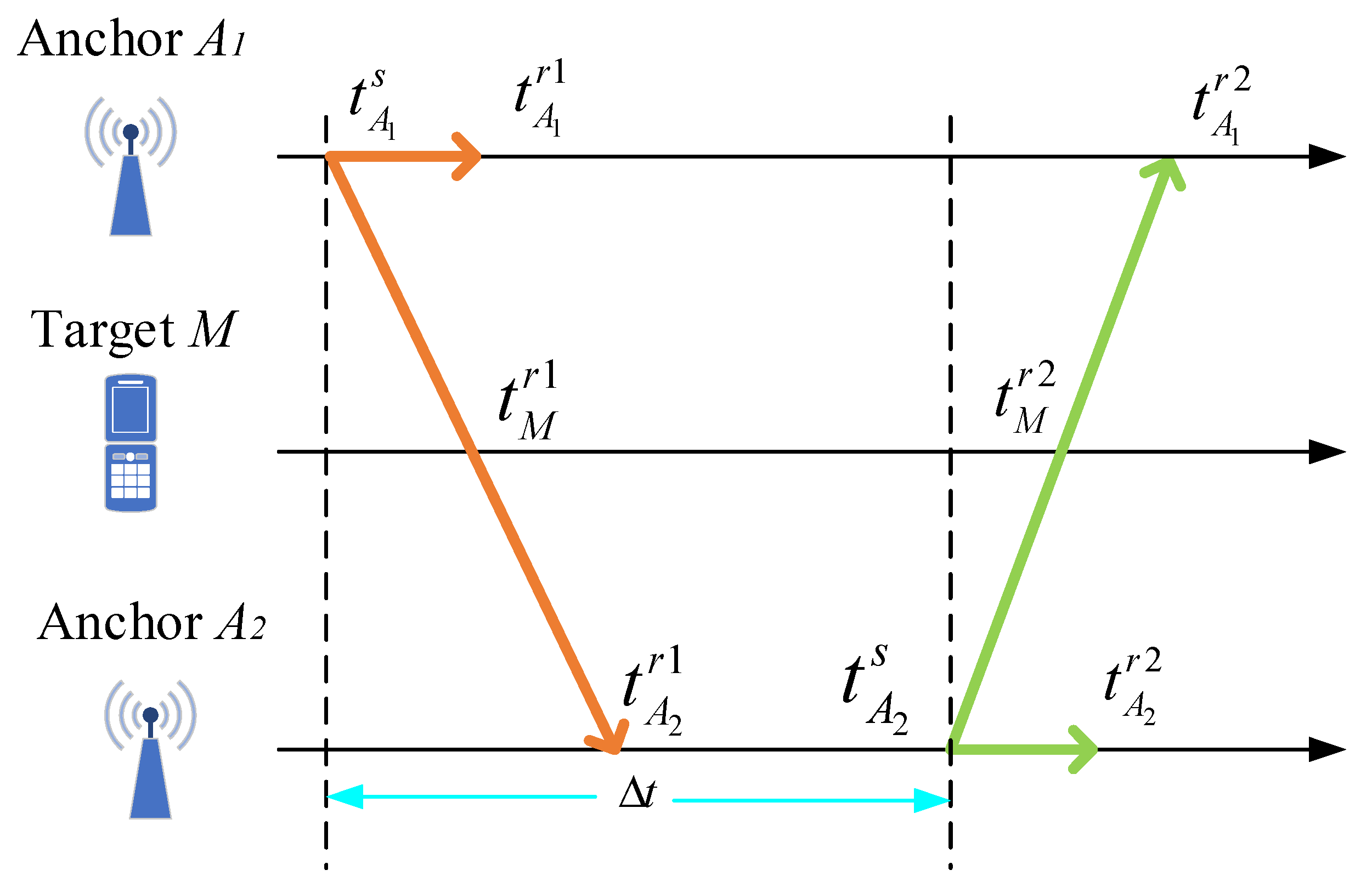
We detail the TDOA estimation for the ultrasonic localization in Figure 4. Let the system comprise anchors A1 and A2 and target M.
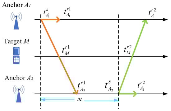
Figure 4.
Diagram of message transmission and reception between two anchors and one target.
Suppose at time anchor A1 transmits a message that arrives at anchor A1, A2 and M at and , respectively. At time , anchor A2 sends a message, which is received at times and , respectively. Here, it is unknown for and .
Consider to be the transmission interval between anchors A1 and A2 in a common reference time and and to be the distances from anchor A1’s speaker to the microphone and anchor A2’s speaker to the microphone, respectively. We use to express the distance from anchor Ai’s speaker to anchor Aj’s microphone. Let c be the speed of acoustic propagation in the air.
We can obtain the timestamps t1 and t2 at which anchor A2 sends messages from anchors A1 and A2
The timestamps t3 and t4 at which anchor A1 sends messages from anchors A1 and A2 are obtained separately
Therefore, the transmission interval can be expressed as follows:
Then, it can be further simplified as
After determining the transmission interval , the TDOA from anchors A1 and A2 on target M can be calculated. The time calculations are all based on the same device clock system for time subtraction. Therefore, the distances difference from anchors A1 and A2 to target M can be computed as
where c is the speed of acoustic signal propagation in the atmosphere.
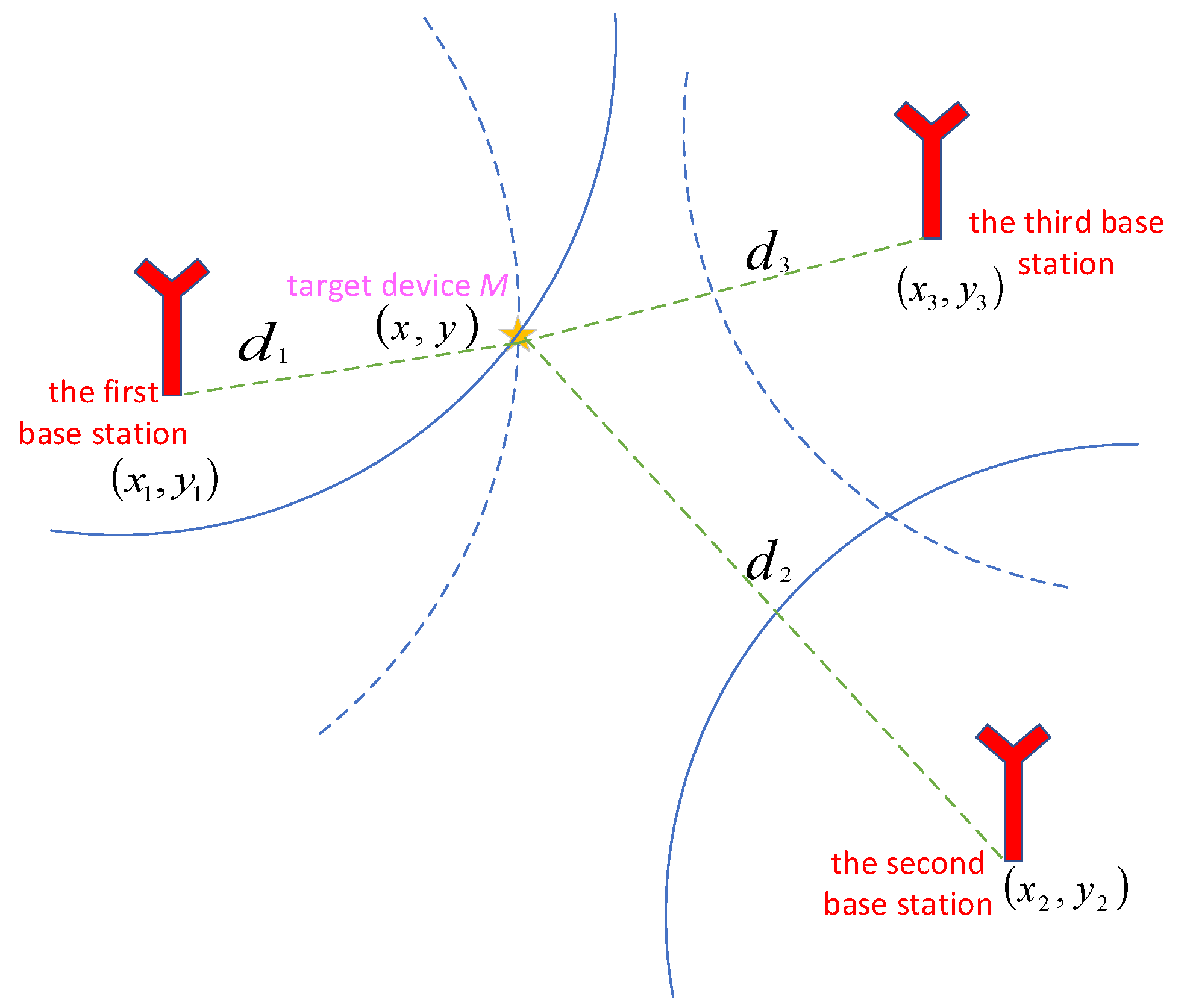
At least three anchors are needed to achieve localization in the location estimation. The TDOA hyperbolic model [38] is shown in Figure 5. We assume the target location and anchor locations , . is the distance difference from anchors Ai and Aj on Target M. The location can be achieved by using Equation (9).
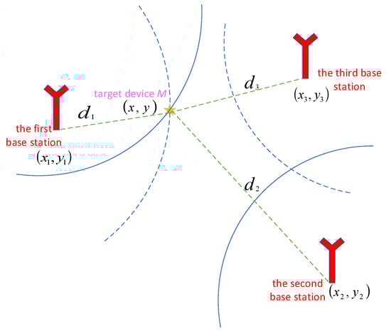
Figure 5.
TDOA hyperbolic model.
Suppose Ai’s location is . Then, the distance between the target M and anchor Ai is
where .
Let denote the distance difference from anchors Ai and A1 on Target M then
We can obtain
Equation (13) can be expanded and expressed as
When i = 1, Equation (11) simplifies to
Equation (14) is subtracted from Equation (15) to obtain
where ,.
From Equation (16), we obtain
Then, we can obtain the matrix
where
The location can be computed as
4.3.2. Improved Pedestrian Dead Reckon Estimation
In this part, we elaborate on the improved pedestrian dead reckoning algorithm, which includes step length estimation, heading direction, and dead reckon estimation.
- Step length estimation
While walking, the acceleration of the pedestrian changes approximately periodically. The alternating transformation of the peak and valley of the acceleration wave once is equivalent to one step, so peak detection can be used to estimate the step frequency and step length. The detection process is mainly divided into the following three parts:
- (1)
- Peak detection:
If the acceleration at time t is greater than the acceleration at time and at time , then is considered the peak.
- (2)
- Threshold setting:
To ensure the validity of these peaks and valleys, the peak threshold is set. If the detected peak is less than the preset peak threshold, it will be discarded.
- (3)
- Step determination:
If , the peak is recorded as a valid peak. is the time of the (i − 1)-th step, and is the training value of the time taken by the pedestrian to walking one step.
The step detection algorithm is depicted in Algorithm 1.
| Algorithm 1: Step Detection Algorithm |
| Input: Acceleration sequence . |
| Output: i-th step . |
| 1: Setting Threshold and one-step taken time ; |
| 2: for i = 1: do |
| 3: if is the Peak value then |
| 4: if and - then |
| 5: |
| 6: end if |
| 7: end if |
| 8: end for |
While walking, the step length in the current state is not only related to the current acceleration but also to the previous acceleration. It is not accurate to estimate the step length considering only the current motion state.
Inspired by the literature [39], our method is not only related to the peak and valley values of acceleration in the current step but also accounts for the previous two steps. It can reflect the continuity and similarity of the moving process. Due to equipment errors during acceleration acquisition, we have added to compensate for the error caused by the equipment in the step length estimation. Meanwhile, during the estimation process, the attention mechanism scheme is also adaptively designed by calculating the difference between the maximum and minimum values of acceleration within each step, which has better adaptability than fixed weight estimation.
The improved step length estimation method integrates the previous two step lengths as follows:
where , are the (i − 1)-th and (i − 2)-th step length, respectively is the weighting vector, K is the model parameter, and are the peak and valley values of the acceleration in the i-th step, and is the accelerometer compensation, which is measured at a stationary time.
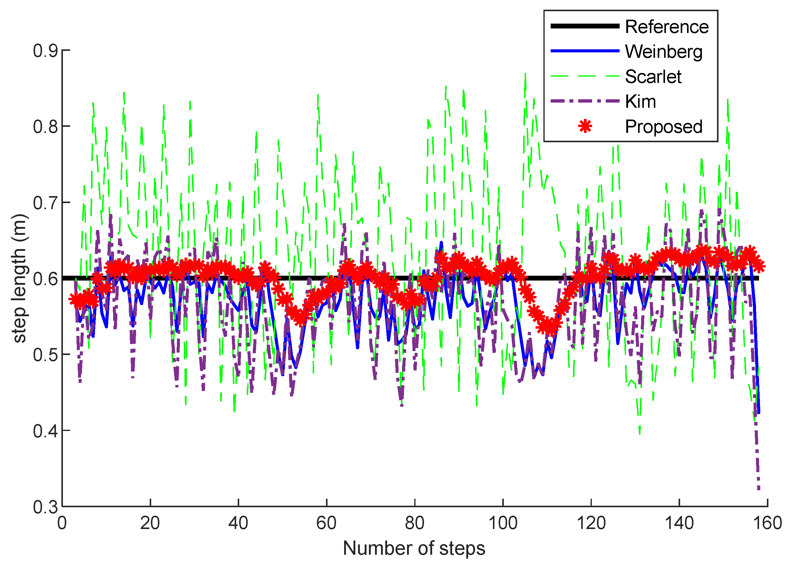
Tests with several static states have been conducted in experiments. We have carried out some experiments with Scarlet [40], Kim [41], Weinberg [42] and our method. Figure 6 shows the comparison of the step length estimation at the trial site when the pedestrians walk at 0.6 m per step. The mean step length of our improved step model is 0.5939 m. The mean step lengths of the Weinberg, Scarlet, and Kim models are 0.5645 m, 0.6228 m, and 0.5567 m, respectively. The experimental results show that our method has higher stability and accuracy. This result is mainly due to the improved method, which can extract more features related to the current step than the Scarlet, Kim, and Weinberg methods. At the same time, the different attention values of each step are calculated adaptively and can predict more accurate pedestrian states.
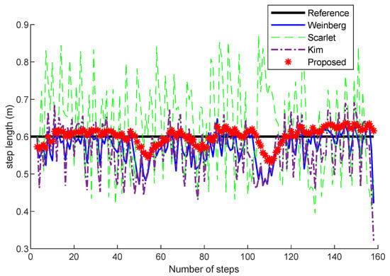
Figure 6.
Comparisons of step length estimation at different step numbers with Scarlet, Kim, Weinberg and the proposed method.
- Heading direction estimation
According to Euler’s theorem, the quaternion-based attitude matrix description [43] is the transformation of the target coordinate system to the Earth coordinate system, as shown in Equation (24),
where denotes the rotation matrix of the quaternions. denotes the posture quaternion, which is the unit vector, is the quaternion coefficient of the scalar part, whose value is equal to the cosine of half of the rotation angle of the coordinate system, denote the part of the vector, and satisfied the following constraint:
Since the gyroscope data can be used to estimate the heading angle from the differential equations of motion and gravitational acceleration and geomagnetic intensity can be used to correct the heading angle, the extended Kalman filter (EKF) is used to estimate the heading angle. The equation of state and the measurement equation of the EKF are expressed as Equations (26) and (27). The state vector is represented by the quaternion , and the measurement equation is a combination of the acceleration and magnetometer measurement data.
where and measured by the acceleration and magnetometer sensors at time k, respectively, is the state transfer matrix, is the process noise, and is the measurement noise. is the attitude rotation matrix, is the normalized gravity vector, and is the normalized magnetic field strength vector.
After the EKF prediction update, the optimal state vector can be iterated for each moment then the estimated optimal heading angle is as shown in Equation (28).
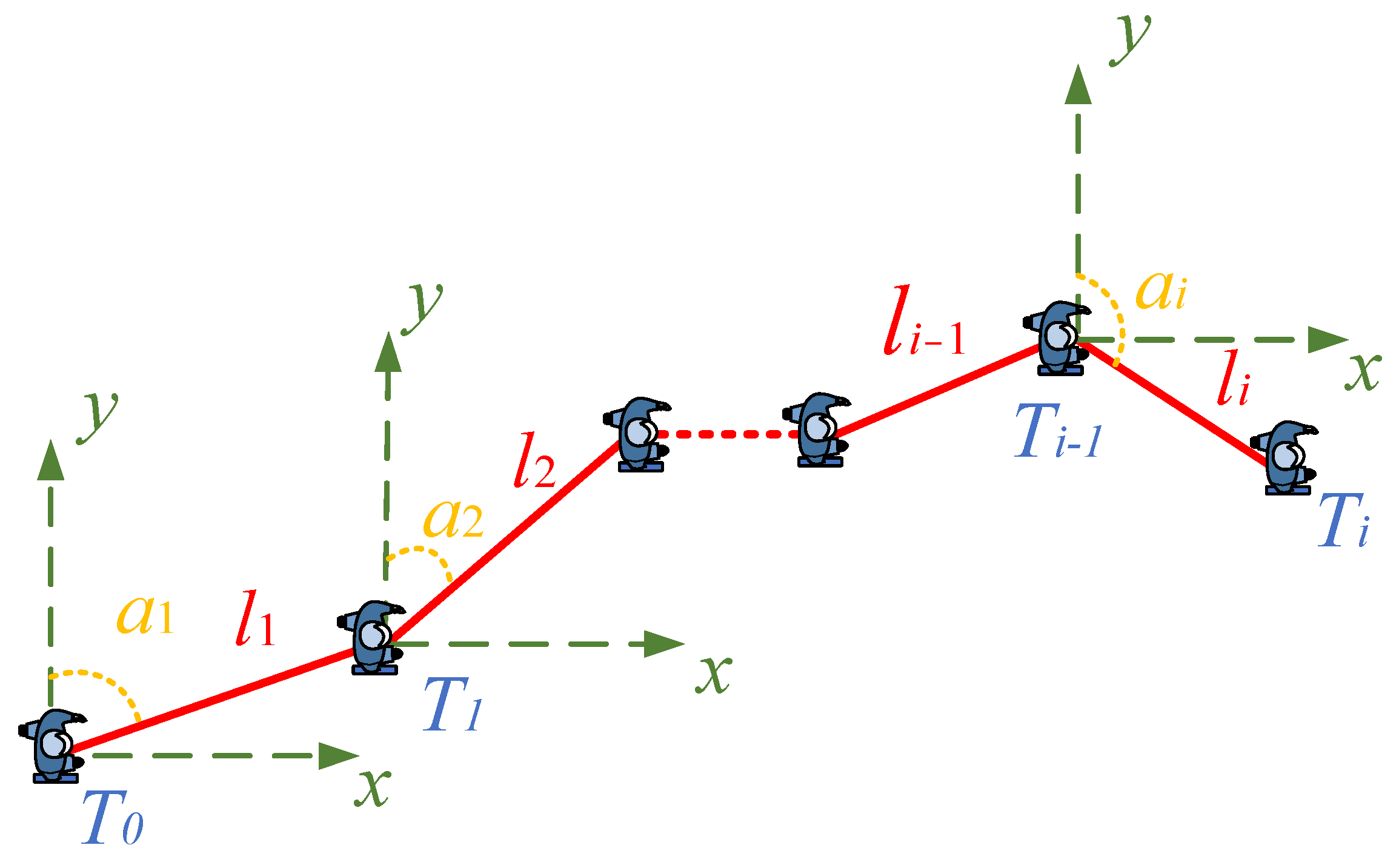
- Dead reckoning
The dead reckon schematic diagram (considering only the two-dimensional case) is shown in Figure 7.
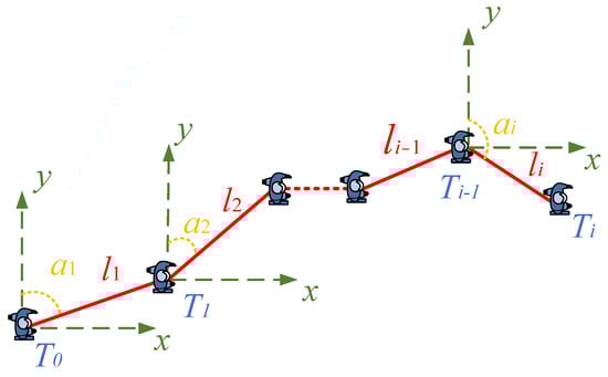
Figure 7.
PDR motion model diagram.
Therefore, the current location for the i-th step can be estimated according to the previous step, step length and heading direction. It is computed by the following formula:
where is the i-th step length and indicates the heading direction of the i-th step.
4.4. Adaptive Weight Value Generation
We propose an adaptive weight value generation scheme for acoustic signal estimation and IMU estimation. The weight value mechanism generates larger values for the important estimation and smaller values for the others. By generating the weight value, more generality and accuracy can be achieved.
Suppose at time k, given the location for TDOA estimation and for the IMU, at time k − 1, the location is .
For TDOA estimation, the distance for the current and previous times can be calculated as
For IMU estimation, the distance for the current and previous time can be calculated as
We can obtain , .
The normalized weights for time k can be obtained as
After normalization, the sum of the weight values is 1.
4.5. Localization Estimation of the Fusion Method
In fusion localization, TDOA estimation is used to determine the initial location. To ensure accuracy, the optimal location is chosen by many trial tests.
Weight value generation can obtain the importance vectors. Formally, the weight value is defined as follows
where and are the estimated weight values of the TDOA and improved PDR methods, respectively.
Based on the estimation location from the two modules and the corresponding important values, we can estimate the current location at time k as follows
where W is the weight values.
However, due to the interferences of noise, multipath effects, and other factors, anomaly estimation is inevitable. During fusion localization, four cases occur. We propose setting the distance threshold scheme, which is adaptively adjusted according to the current and previous location. Experiments demonstrate that it is feasible to adopt 1.5 times the distance of the current location and estimation location. These cases are as follows:
Case 1: If the distance for the TDOA estimation is greater than the threshold: , the estimation by the TDOA method may be an outlier and discarded. Then, the estimation of the PDR method is adopted for localization, that is, .
Case 2: If the distance for the PDR estimation is greater than the threshold: , the estimation by the PDR method may be an outlier and discarded. Then, the estimation of the TDOA method is more accurate; therefore, .
Case 3: If the distance for the PDR and TDOA estimation is greater than the thresholds and , the estimations are anomaly location. Return to estimate target.
Case 4: The distance for the PDR and TDOA estimation is less than the threshold: and . Then, fusion localization will perform.
5. Illustrative Experimental Results
To evaluate the performance of our proposed multimodal fusion system, we conducted extensive experiments at three different experimental sites, which include a 35 × 16 × 3 m3 area and a 12 × 8 × 3 m3 area and 11 × 9 × 3 m3 area. Figure 8 shows the floorplans of these trial sites. Covering 560 m2, the first scene includes open spaces. The second scene covers approximately 96 m2, is relatively small and includes some tables and chairs. The third scene covers approximately 99 m2, is relatively small and includes some tables, chairs, and cabinet. First, we detail the experimental setting in Section 5.1. Then, the discussion and analysis are provided in Section 5.2, and finally, we illustrate the localization results in Section 5.3.
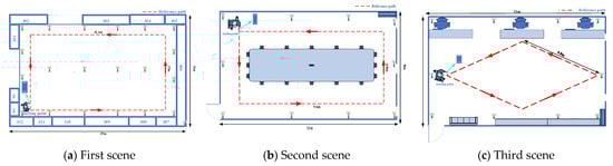
Figure 8.
Floorplans of the experimental sites: (a) scene 1 with open spaces, (b) scene 2 includes small spaces with some tables and chairs, (c) scene 3 includes small spaces with some tables, chairs and cabinet.
5.1. Experimental Setting
We have developed the acoustic and inertial fuse localization system, which includes a client application and a server program. The client application was installed on Android devices with IMU sensors. The server program was installed on a 64-bit work station with a Windows operating system.
Client application: The client was developed using the Android operating system. The pedestrian carries the mobile phone with installed the client application to capture accelerometer, gyroscope, and directional angle readings as they walk. During the data collection process, it not only records the time stamp when the sensor readings are taken but also collects the signals from the anchor nodes placed in different locations around the experimental trial sites.
Server program: The localization program is implemented on the work station, which employed a Windows operating system with 64 bits. After receiving sufficient data, they will be sent to the server. The server program extracts the ultrasonic and inertial sequences separately. The coarse determination is conducted using the acoustic and inertial sequences. Then, the fusion localization estimation is achieved based on the adaptive weight value with coarse determination.
At the first experimental trial site, twenty anchor nodes for periodically transmitting acoustic signals were installed, and the mobile device was used as the localization target. At the second and third experimental trial sites, ten anchors were installed as acoustic sources.
In these experiments, we invited five volunteers to collect acoustic and IMU data. During walking, the volunteers move along the designated route with the target smartphone in hand, and the client program automatically collected acoustic and sensor readings.
5.2. Discussion and Analysis
5.2.1. Step Length Estimation
To validate the effect of step detection at different walking speeds, we ask a volunteer to hold smartphone and walk along the survey path at slow, normal and fast speed. During walking, the mobile device points in the head direction, and the client collects the sensor’s data automatically. For three cases, the volunteer has collected five trial data, respectively.
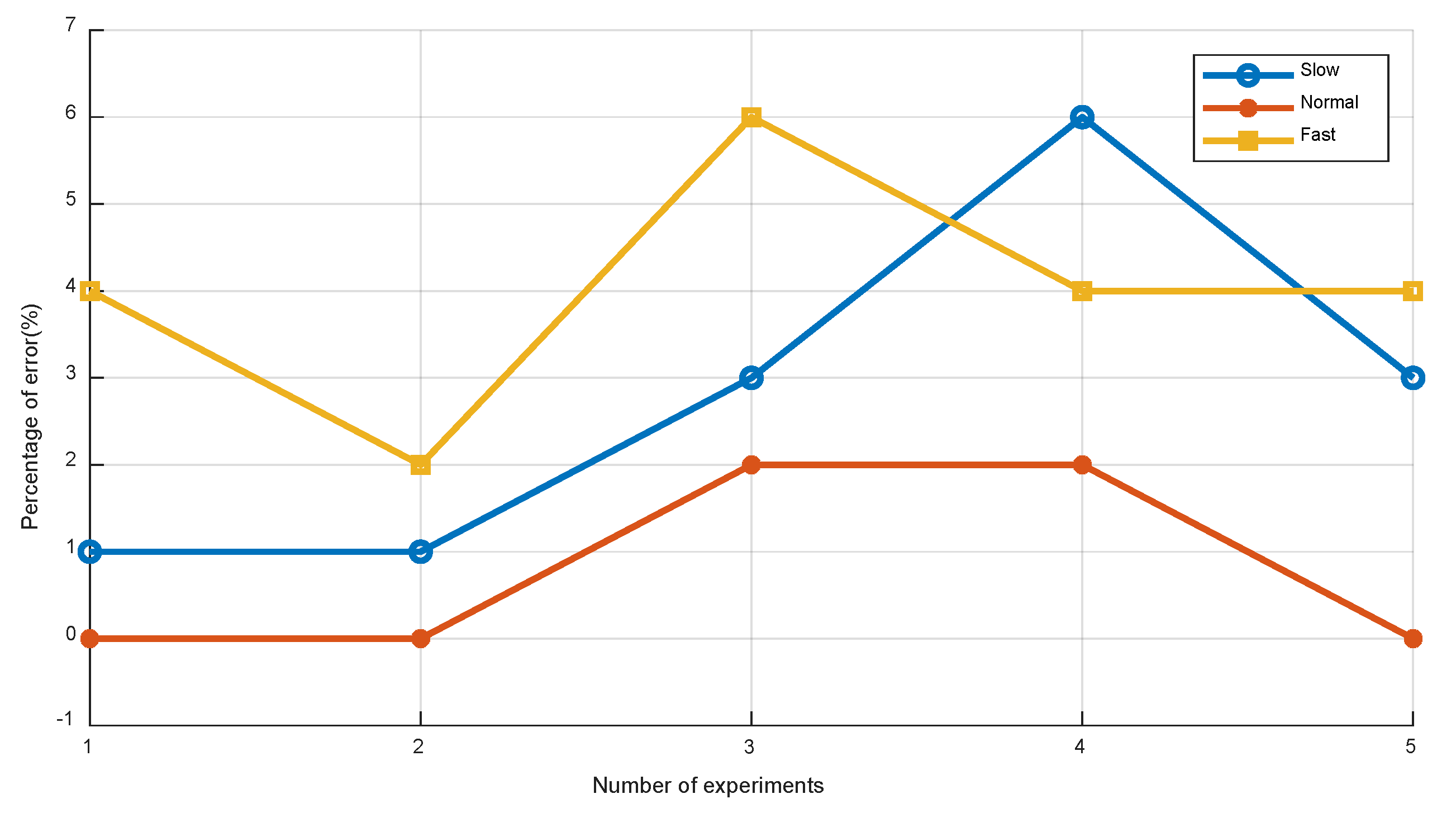
Figure 9 shows the step number error at slow, normal, and fast speeds. It can be seen that the step detection can achieve better performance when the user walks at normal speed. This is due to the fact that the fluctuation of the acceleration is smaller and wave crests may be missed when the pedestrian walks at slow walking speeds. The fluctuation in the acceleration becomes greater at faster speeds, and the peaks and valleys may be misdetected, which results in an overchecked step count. Therefore, in our experiments, we let the pedestrians walk at a normal speed.
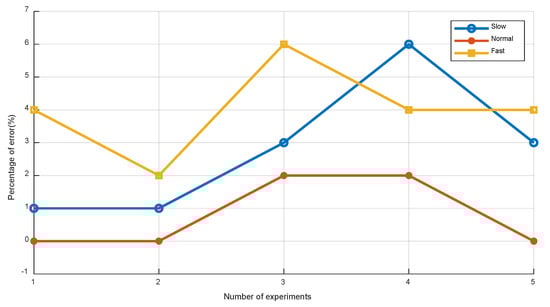
Figure 9.
Step number error at different walking speeds.
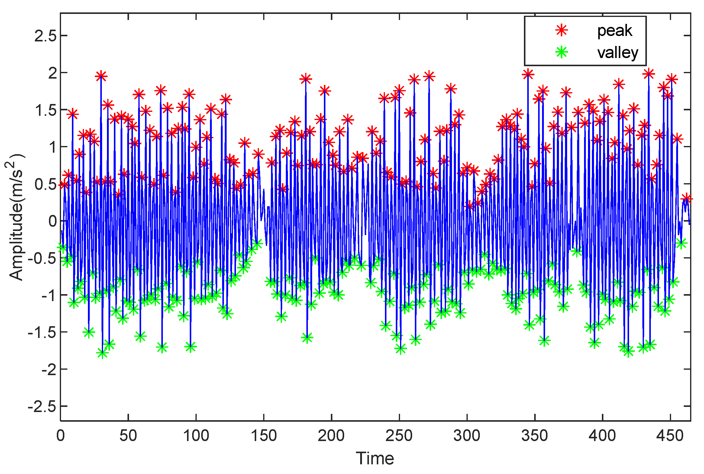
In the step length estimation, the volunteer walks at normal speed and collects the IMU data. Figure 10 shows the peak detection results for the pedestrians in which the peaks and valleys of acceleration are labeled with red and green stars, respectively. This figure shows that all of the peaks and valleys in the acceleration are detected and can be achieved with high accuracy.
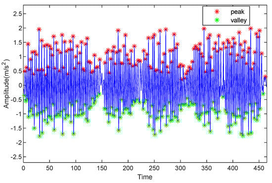
Figure 10.
Peak and valley detection of acceleration.
In this paper, we conducted experiments with the improved step length estimation at the trial site. Five volunteers are recruited and asked to collect data while walking along a corridor totaling 30 m with their cell phones in hand. Ten sets of IMU data are captured each time. Table 1 shows the solution distances and errors corresponding to each volunteer. The experimental results demonstrate that the improved step length method can achieve more accurate than the traditional algorithm, and the errors are not greater than 1.5%. The improved method has more pervasiveness.

Table 1.
Comparison results between the Weinberg method and proposed step length estimation method (m).
5.2.2. Improved PDR Estimation Results
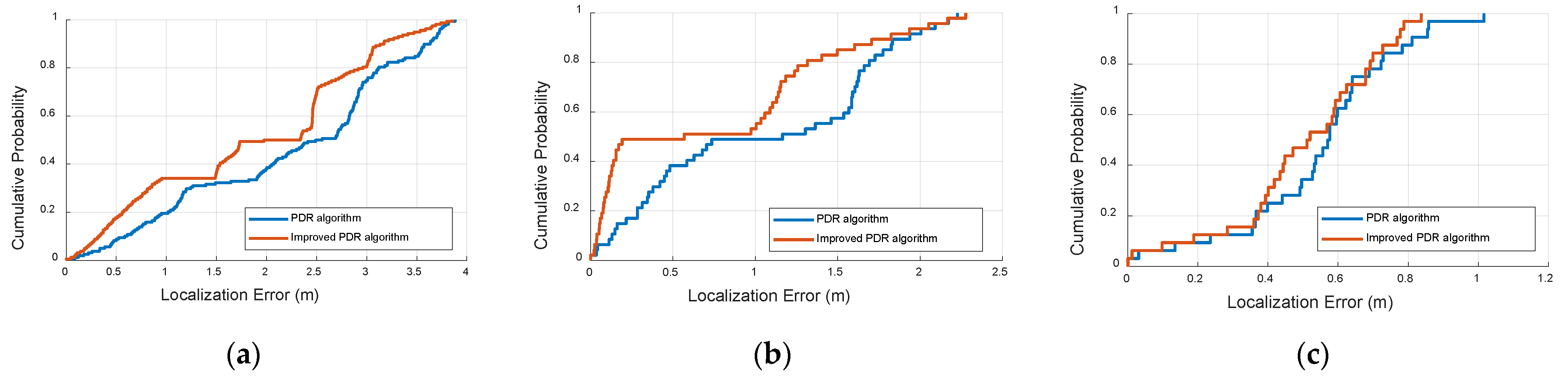
Figure 11 illustrates the cumulative density function (CDF) of the localization error for the traditional PDR method and improved PDR method in the three scenes, in which the abscissa is the localization error, the unit is meter, and the ordinate is the corresponding CDF. Figure 11 shows that the proposed method has a smaller localization error than the PDR method, which occurs due to the fact that our method can extract more features from the IMU data to improve the localization estimation.
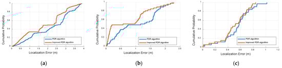
Figure 11.
CDF of localization errors between the improved PDR and traditional PDR method at three sites. (a) First scene, (b) Second scene, (c) Third scene.
5.3. Localization Performance
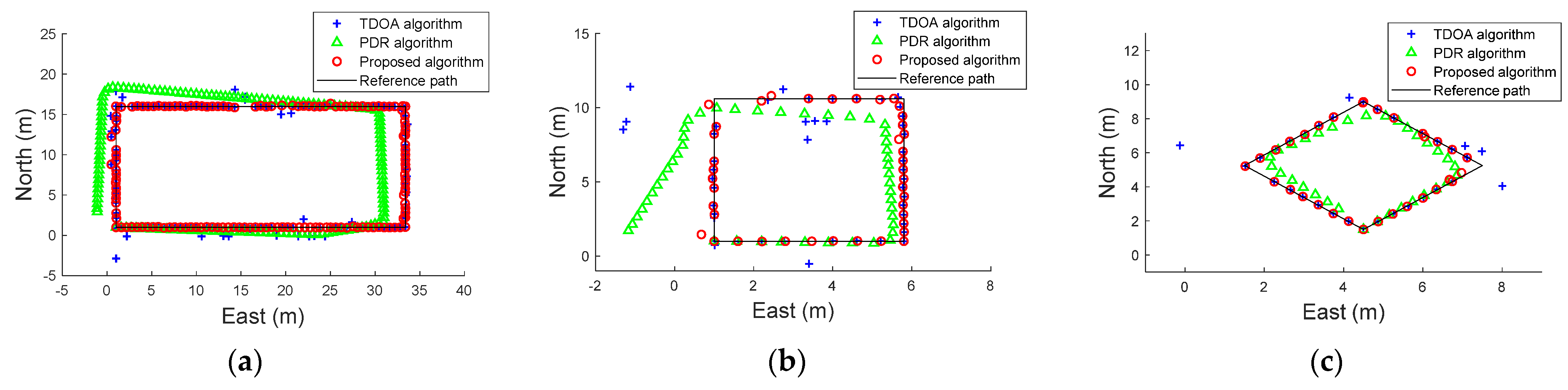
In this section, we conducted a localization experiment on the global region in the three scenes. The user walks along all of the planned paths in the whole scene to collect the IMU data and acoustic signals. Figure 12 shows the localization results using different algorithms. The TDOA estimation based acoustic signals can achieve good accuracy. However, some anomaly points occur. The errors in the PDR estimation increase over time, and the localization path increasingly deviates from the original path. The experiments indicate that the proposed method can achieve better localization estimation at the different planned paths than state-of-the-art algorithms. This is mainly due to the following two reasons. First, we introduce the threshold detection scheme into fusion localization, which can effectively suppress the anomaly points of TDOA outliers and the cumulative error of PDR estimation. In addition, the weight value generation can be of greater importance in TDOA and PDR estimations than the fixed weight value.
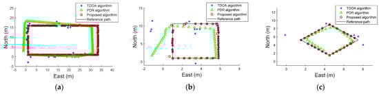
Figure 12.
Localization track map with TDOA algorithm, PDR algorithm and proposed algorithm at three experimental sites. (a) First scene, (b) Second scene, (c) Third scene.
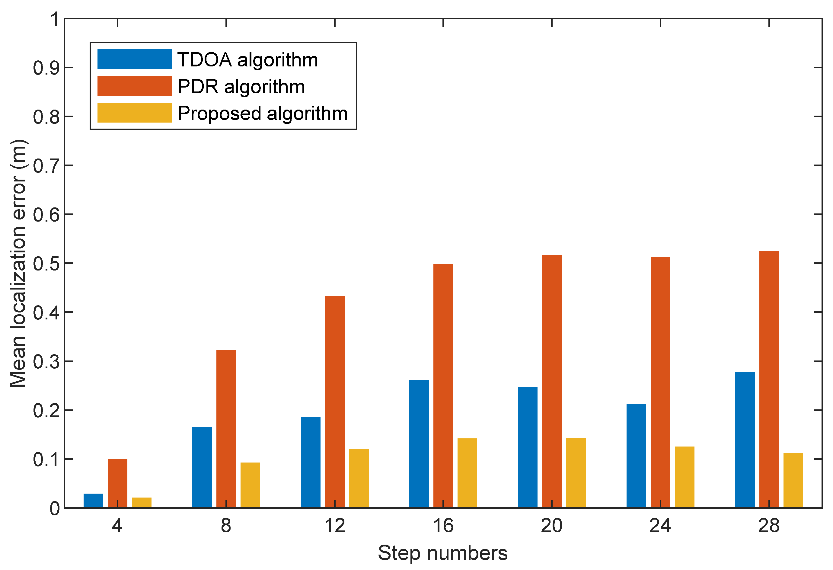
We compare the mean localization errors among TDOA, PDR, and the proposed algorithm with different step numbers at three scenes in Figure 13, Figure 14 and Figure 15. They show that the mean localization errors for the TDOA method are generally stable. Specifically, the proposed algorithm does not vary significantly in localization accuracy with different travel paths. The mean localization for the PDR algorithm has an increasing localization error over time due to the cumulative error. Compared with the TDOA and PDR algorithms, our proposed fusion algorithm has the smallest mean localization error. This is due to the fact that our proposed threshold value based on step size removes the anomalies generated by acoustic signal localization, and acoustic signal localization corrects the problem of the cumulative errors generated by PDR localization.
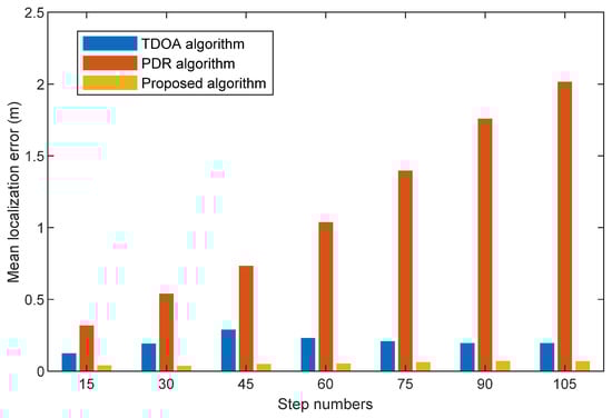
Figure 13.
Mean localization error comparison with TDOA algorithm, PDR algorithm, and the proposed algorithm at different step numbers (First scene).
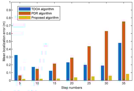
Figure 14.
Mean localization error comparison with TDOA algorithm, PDR algorithm, and the proposed algorithm at different step numbers (Second scene).
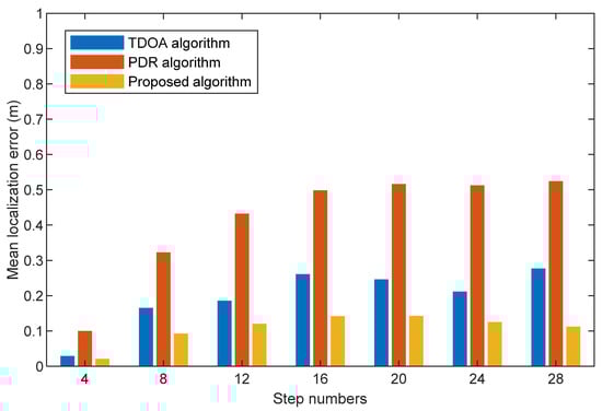
Figure 15.
Mean localization error comparison with TDOA algorithm, PDR algorithm, and the proposed algorithm at different step numbers (Third scene).
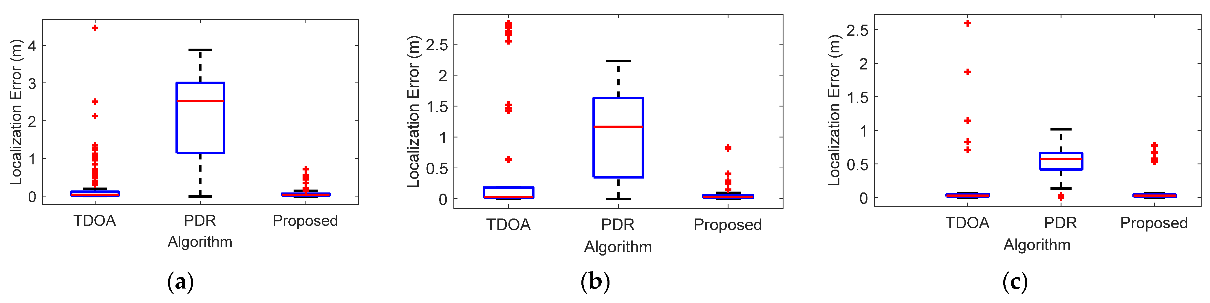
We present the localization errors incurred at the three trial sites in Figure 16. The experiment illustrates that the proposed method achieves comparable localization accuracy. The fusion scheme has an effective method to gain enough information. Consequently, it is able to detect the anomalies and cumulative errors caused by PDR localization.
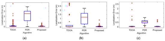
Figure 16.
Localization error with TDOA algorithm, PDR algorithm and the proposed algorithm at different scenes. (a) First scene, (b) Second scene, (c) Third scene.
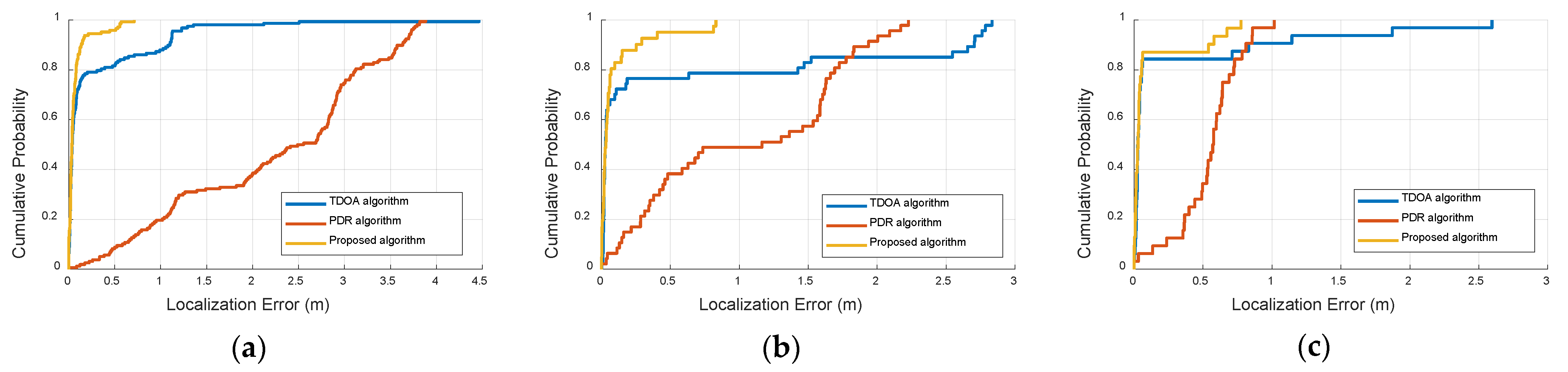
Figure 17 illustrates the cumulative density function (CDF) of the localization error in the three scenes, where the abscissa is the localization error, the unit of measurement is meters, and the ordinate is the corresponding CDF. From Figure 17a, it can be seen that the TDOA estimation is approximately 0.35 m when the accumulative probability accuracy is 80%. The PDR estimation is above 3.12 m when the accumulative probability accuracy is 80%. The proposed algorithm is approximately 0.08 m when the accumulative probability accuracy is 80%. It is therefore shown that the proposed method has better localization performance than TDOA and PDR estimation. From Figure 17b, it can be seen that the TDOA estimation is approximately 1.43 m when the accumulative probability accuracy is 80%, and the PDR estimation is above 1.69 m when the accumulative probability accuracy is 80%. The proposed algorithm is approximately 0.07 m when the accumulative probability accuracy is 80%. From Figure 17c, it can be seen that the TDOA estimation is approximately 0.06 m when the accumulative probability accuracy is 80%, and the PDR estimation is above 0.72 m when the accumulative probability accuracy is 80%. The proposed algorithm is approximately 0.05 m when the accumulative probability accuracy is 80%. These results show that the proposed fusion algorithm achieves sufficient accuracy compared with the state-of-the-art algorithms. This is due to the fact that the weight value generation can adaptively identify the importance between the TDOA estimation and PDR estimation. The threshold schemes can detect effective outliers.
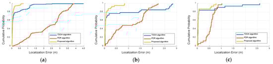
Figure 17.
CDF of localization errors with TDOA algorithm, PDR algorithm and the proposed algorithm at different scenes. (a) First scene, (b) Second scene, (c) Third scene.
Table 2, Table 3 and Table 4 demonstrate the mean error and root mean squared error (RMSE) of the different localization methods at the trial sites. In the first scene, the mean error and RMSE of our method are 0.0704 m and 0.139 m, respectively. In the second scene, the mean error and RMSE of our method are 0.094 m and 0.2066 m, respectively. In the third scene, the mean error and RMSE of our method are 0.1041 m and 0.2348 m, respectively. For the three sites, these values show that the localization performances in the proposed fusion localization have been greatly improved, which occurs since the proposed method can supply sufficient information about anomalies, effectively eliminate the errors, and guarantee the fluctuation of the localization estimation around the real value.
Table 2.
Comparison of localization accuracy with different algorithms (m) (First scene).
Table 3.
Comparison of localization accuracy with different algorithms (m) (Second scene).
Table 4.
Comparison of localization accuracy with different algorithms (m) (Third scene).
Table 5, Table 6 and Table 7 show the four percentile of error magnitude at 0.5, 0.75, 0.9, and 0.95 for the three trial sites. The experimental results illustrate that the proposed method has better localization performance at different walking paths in these indoor scenes than the state-of-the-art methods. This is due to the fact that the fusion scheme is able to provide effective information for localization.
Table 5.
Comparison of quantiles of error with different algorithms (m) (First scene).
Table 6.
Comparison of quantiles of error with different algorithms (m) (Second scene).
Table 7.
Comparison of quantiles of error with different algorithms (m) (Third scene).
6. Conclusions
In this paper, to solve the problem of anomalies in acoustic signal localization, we propose a step threshold method that can set the threshold value based on the step length of the previous step and thus solve the anomalies in localization. Then, in the PDR localization system, we improve the traditional step estimation algorithm model and propose an improved model that adaptively estimates the current step length based on the previous two-step length and the current acceleration value. Finally, we fuse acoustic estimation and improved PDR estimation to achieve the pedestrian’s location by generating distance weights. An indoor localization system by fusing the TDOA and improved PDR estimation is achieved high localization performance and low cost. We have conducted extensive experiments at three sites. The experimental results demonstrate that the average localization error of our method achieves higher accuracy compared with the state-of-the-art algorithms. Considering the compatibility of mobile phones with ultrasonic and inertial signals, our localization system has a relatively low cost.
Author Contributions
Conceptualization, S.Y.; Data curation, C.W.; Formal analysis, H.D.; Funding acquisition, S.Y. and J.X.; Methodology, H.D. and J.X.; Project administration, Y.J.; Resources, X.L.; Software, X.L.; Writing—original draft, C.W.; Writing—review & editing, Y.J. All authors have read and agreed to the published version of the manuscript.
Funding
This work was supported in part by National Natural Science Foundation of China: Grant 62061010, Grant 62161007, Grant 61936002, Grant 2018AAA0100300 and Grant 6202780103; Guangxi science and Technology Project: Grant AA19254029, Grant AA20302022 and Grant AB21196041; Nanning City Qingxiu District Science and Technology Major Special Project: Grant 2018001; Guilin Science and Technology Project: Grant 20210222-1; Innovation Project of Guang Xi Graduate Education: YCSW2022291.
Institutional Review Board Statement
Not applicable.
Informed Consent Statement
Not applicable.
Data Availability Statement
All test data mentioned in this paper will be made available on request to the corresponding author’s email with appropriate justification.
Conflicts of Interest
The authors declare no conflict of interest.
Notations
| The time when anchor Ai transmits a message | |
| The time when anchor Aj receive the message from anchor Ai | |
| The transmission interval between anchors | |
| The distance from anchor Ai’s speaker to anchor Aj’s microphone | |
| The distance difference from anchors Ai and Aj on Target | |
| The distance between the target M and anchor Ai | |
| The scalar part of the quaternion coefficients | |
| The vector part of the quaternion coefficient | |
| The state vector at time k | |
| The acceleration measured by the accelerometer at time k | |
| The data measured by the magnetometer sensor at time k | |
| The location estimation at time k | |
| The location estimation using TDOA method at time k | |
| The location estimation using PDR method at time k | |
| The distance between the current and previous time using TDOA method | |
| The distance between the current and previous time using PDR method | |
| Weight value in TDOA method at time k | |
| Weight value in PDR method at time k | |
| Weight value in TDOA method | |
| Weight value in TDOA method | |
| Distance threshold |
References
- Wu, W.; Fu, S.; Luo, Y. Practical Privacy Protection Scheme In WiFi Fingerprint-based Localization. In Proceedings of the 2020 IEEE 7th International Conference on Data Science and Advanced Analytics (DSAA), Sydney, NSW, Australia, 6–9 October 2020; pp. 699–708. [Google Scholar]
- Gong, P.; Wei, D.; Ji, X.; Li, W.; Yuan, H. Research on Geomagnetic Matching Localization for Pedestrian. In Proceedings of the China Satellite Navigation Conference (CSNC) 2018 Proceedings; Springer: Singapore, 2018; pp. 537–549. [Google Scholar] [CrossRef]
- Fischer, G.; Bordoy, J.; Schott, D.J.; Xiong, W.; Gabbrielli, A.; Hoflinger, F.; Fischer, K.; Schindelhauer, C.; Rupitsch, S.J. Multimodal Indoor Localization: Fusion Possibilities of Ultrasonic and Bluetooth Low-Energy Data. IEEE Sens. J. 2022, 22, 5857–5868. [Google Scholar] [CrossRef]
- Shen, M.; Wang, Y.; Jiang, Y.; Ji, H.; Wang, B.; Huang, Z. A New Positioning Method Based on Multiple Ultrasonic Sensors for Autonomous Mobile Robot. Sensors 2019, 20, 17. [Google Scholar] [CrossRef] [PubMed] [Green Version]
- Caicedo, D.; Pandharipande, A. Ultrasonic Arrays for Localized Presence Sensing. IEEE Sens. J. 2012, 12, 849–858. [Google Scholar] [CrossRef]
- Franz, W.; Gunther, A.; Bernhard, H.-W. A pedestrian navigation system for urban and indoor environments. In Proceedings of the 20th International Technical Meeting of the Satellite Division of The Institute of Navigation (ION GNSS 2007), Fort Worth, TX, USA, 25–28 September 2007; pp. 1380–1389. [Google Scholar]
- Chen, G.; Zhang, Y.; Yang, Z. A pedometer implementation method based on mobile phone sensor autocorrelation analysis. J. Chin. Inert. Technol. 2014, 22, 794–798. [Google Scholar] [CrossRef]
- Yao, Y.; Pan, L.; Fen, W.; Xu, X.; Liang, X.; Xu, X. A Robust Step Detection and Stride Length Estimation for Pedestrian Dead Reckoning Using a Smartphone. IEEE Sens. J. 2020, 20, 9685–9697. [Google Scholar] [CrossRef]
- Wang, J.; Hu, A.; Liu, C.; Li, X. A Floor-Map-Aided WiFi/Pseudo-Odometry Integration Algorithm for an Indoor Positioning System. Sensors 2015, 15, 7096–7124. [Google Scholar] [CrossRef] [Green Version]
- Chen, G.; Li, F.; Zhang, Y. A MEMS step counting algorithm based on adaptive peak detection. J. Chin. Inert. Technol. 2015, 23, 315–321. [Google Scholar] [CrossRef]
- Wang, H.; Wang, X.; Xue, Y.; Jiang, Y. UWB-based Indoor Localization Using a Hybrid WKNN-LSTM Algorithm. In Proceedings of the 4th IEEE Information Technology, Networking, Electronic and Automation Control Conference (ITNEC), Chongqing, China, 12–14 June 2020; pp. 1720–1725. [Google Scholar]
- Nakamura, A.; Naoto, S.; Makoto, I. Performance Analysis of UWB Positioning System at the Crossing. In Proceedings of the 21st IEEE International Conference on Intelligent Transportation Systems (ITSC), Maui, HI, USA, 4–7 November 2018; pp. 786–791. [Google Scholar]
- Jiménez, A.R.; Seco, F. Comparing Decawave and Bespoon UWB location systems Indoor outdoor performance analysis. In Proceedings of the 2016 International Conference on Indoor Positioning and Indoor Navigation (IPIN), Alcala de Henares, Spain, 4–7 October 2016; pp. 1–8. [Google Scholar]
- Zhu, W. Research on WiFi Location Technology Based on Location Fingerprintg. China Comput. Commun. 2021, 2, 14–16. [Google Scholar]
- Hernández, N.; Parra, I.; Corrales, H.; Izquierdo, R.; Ballardini, A.L.; Salinas, C.; García, I. WiFiNet: WiFi-based indoor localisation using CNNs. Expert Syst. Appl. 2021, 177, 114906. [Google Scholar] [CrossRef]
- Jia, B.; Huang, B.; Gao, H.; Li, W.; Hao, L. Selecting Critical WiFi APs for Indoor Localization Based on a Theoretical Error Analysis. IEEE Access 2019, 7, 36312–36321. [Google Scholar] [CrossRef]
- Yang, B.; Yang, E. A Survey on Radio Frequency based Precise Localisation Technology for UAV in GPS-denied Environment. J. Intell. Robot. Syst. 2021, 103, 38. [Google Scholar] [CrossRef]
- Shen, L.; Zhang, Q.; Pang, J.; Xu, H.; Li, P.; Xue, D. ANTspin: Efficient Absolute Localization Method of RFID Tags via Spinning Antenna. Sensors 2019, 19, 2194. [Google Scholar] [CrossRef] [Green Version]
- Yao, Y.; Bao, Q.; Yao, R.; Xu, X.; Yan, J. BtPDR: Bluetooth and PDR-Based Indoor Fusion Localization Using Smartphones. KSII Trans. Internet Inf. Syst. 2018, 12, 3657–3682. [Google Scholar] [CrossRef]
- Bao, Y.; Zhang, P.; Li, J.; Lu, P. An indoor positioning and navigation technology based on bluetooth. Sci. Surv. Mapp. 2019, 44, 89–95. [Google Scholar]
- Jiang, C.; Liu, J. A smartphone-based indoor geomagnetic positioning system. GNSS Word of China 2018, 43, 9–16. [Google Scholar]
- Wang, Q.; Zhou, J. Simultaneous localization and mapping method for geomagnetic aided navigation. Optik 2018, 171, 437–445. [Google Scholar] [CrossRef]
- Dai, S. The Design and Implementation of Indoor Positioning System Based on Ultrasonic; Southwest Jiaotong University: Chengdu, China, 2017. [Google Scholar]
- Yuan, D.; Zhang, J.; Wang, J.; Cui, X.; Liu, F.; Zhang, Y. Robustly Adaptive EKF PDR/UWB Integrated Navigation Based on Additional Heading Constraint. Sensors 2021, 21, 4390. [Google Scholar] [CrossRef]
- Yuan, Y.; Wang, A.; Jiang, L. Positioning technology with infrared and ultrasonic. Electron. Meas. Technol. 2008, 31, 15–17. [Google Scholar] [CrossRef]
- Li, S.; Sun, H.; Esmaiel, H. Underwater TDOA Acoustical Location Based on Majorization-Minimization Optimization. Sensors 2020, 20, 4457. [Google Scholar] [CrossRef]
- Cui, L.; Song, P. One Optimized Acoustic Localization Algorithm with Temperature Amendment. In Proceedings of the 4th IEEE International Conference on Progress in Informatics and Computing (IEEE PIC), Shanghai, China, 23–25 December 2016; pp. 119–122. [Google Scholar]
- Vakulya, G.; Simon, G. Fast Adaptive Acoustic Localization for Sensor Networks. IEEE Trans. Instrum. Meas. 2011, 60, 1820–1829. [Google Scholar] [CrossRef]
- Manickam, S.; Swar, S.C.; Casbeer, D.W.; Manyam, S.G. Multi-unmanned aerial vehicle multi acoustic source localization. Proc. Inst. Mech. Eng. Part G J. Aerosp. Eng. 2020, 235, 273–294. [Google Scholar] [CrossRef]
- Hu, A.; Deng, Z.; Zhang, Y. Time synchronization algorithm based on improved TPSN and Kalman filtering. Mod. Electron. Tech. 2018, 41, 5–9. [Google Scholar] [CrossRef]
- Wang, Y.-T.; Zheng, R.; Zhao, D. Towards Zero-Configuration Indoor Localization Using Asynchronous Acoustic Beacons. In Proceedings of the 2016 IEEE Intl Conference on Computational Science and Engineering (CSE) and IEEE Intl Conference on Embedded and Ubiquitous Computing (EUC) and 15th Intl Symposium on Distributed Computing and Applications for Business Engineering (DCABES), Paris, France, 24–26 August 2016; pp. 32–39. [Google Scholar]
- Yan, G.; Hou, H.; Luo, Y.; Fang, T.; Wang, W.; Wu, C. High-precision soft clock synchronization method based on TDOA system. Wirel. Commun. 2019, 9, 185–198. [Google Scholar] [CrossRef]
- Liu, K.; Liu, X.; Li, X. Guoguo: Enabling Fine-Grained Smartphone Localization via Acoustic Anchors. IEEE Trans. Mob. Comput. 2016, 15, 1144–1156. [Google Scholar] [CrossRef]
- Lazik, P.; Rowe, A. Indoor pseudo-ranging of mobile devices using ultrasonic chirps. In Proceedings of the 10th ACM Conference on Embedded NetworkSensor Systems, Toronto, ON, Canada, 6–9 November 2012; pp. 99–112. [Google Scholar]
- Cheng, L.; Dai, Y.; Peng, R.; Nong, X. Positioning and navigation of mobile robot with asynchronous fusion of binocular vision system and inertial navigation system. Int. J. Adv. Robot. Syst. 2017, 14, 99–112. [Google Scholar] [CrossRef] [Green Version]
- Cui, J.; Li, B.; Yang, L.; Wu, N. Multi-Source Data Fusion Method for Indoor Localization System. In Proceedings of the 2020 IEEE/CIC International Conference on Communications in China (ICCC), Chongqing, China, 9–11 August 2020; pp. 29–33. [Google Scholar]
- Yadav, R.K.; Bhattarai, B.; Gang, H.-S.; Pyun, J.-Y. Trusted K Nearest Bayesian Estimation for Indoor Positioning System. IEEE Access 2019, 7, 51484–51498. [Google Scholar] [CrossRef]
- Huang, Y. Wireless Location Technology Research Based on TDOA and TOA. Master’s Thesis, Nanjing University of Posts and Telecommunications, Nanjing, China, 2012. [Google Scholar]
- Song, H. Research and Implementation of Indoor Navigation System Based on Pedestrian Dead Reckoning; University of Electronic Science and Technology of China: Chengdu, China, 2018. [Google Scholar]
- Scarlett, J. Enhancing the Perdormance of Pedometers Using a Single Accelerometer; AN-900 Application Note; Analog Devices: Norwood, MA, USA, 2007. [Google Scholar]
- Kim, J.W.; Jang, H.J.; Hwang, D.-H.; Park, C. A Step, Stride and Heading Determination for the Pedestrian Navigation System. J. Glob. Position. Syst. 2004, 3, 273–279. [Google Scholar] [CrossRef] [Green Version]
- Weinberg, H. Using the ADXL202 in Pedometer and Personal Navigation Applications; AN-602 Application Note; Analog Devices: Norwood, MA, USA, 2002. [Google Scholar]
- Renaudin, V.; Combettes, C.; Peyret, F. Quaternion Based Heading Estimation with Handheld MEMS in Indoor Environments. In Proceedings of the 2014 IEEE/ION Position, Location and Navigation Symposium—PLANS 2014, Monterey, CA, USA, 5–8 May 2014. [Google Scholar]


Publisher’s Note: MDPI stays neutral with regard to jurisdictional claims in published maps and institutional affiliations. |
© 2022 by the authors. Licensee MDPI, Basel, Switzerland. This article is an open access article distributed under the terms and conditions of the Creative Commons Attribution (CC BY) license (https://creativecommons.org/licenses/by/4.0/).