Abstract
This article handles tracking multiple targets using bearing-only measurements in underwater noisy environments. For tracking multiple targets in underwater noisy environments, the Gaussian Mixture Probability Hypothesis Density (GM-PHD) filter provides good performance with its low computational load. Bearing-only measurements are passive and do not provide position information of a target. Note that the nonlinearity of the bearing-only measurements can be handled by Extended Kalman Filters (EKF) when applying the GM-PHD filter. However, range uncertainty of the target is large for bearing-only measurements. Thus, a single EKF leads to poor performance when it is applied in the GM-PHD. In this article, every bearing measurement gives birth to multiple target samples, which are distributed considering the feasible range of the passive sensor. Thereafter, every target sample is updated utilizing the measurement update step of the EKF. In this way, we run multiple EKFs associated to multiple target samples, instead of running a single EKF. To the best of our knowledge, our article is novel in tracking multiple targets in noisy environments, using the observer with bearing-only measurements. The effectiveness of the proposed GM-PHD is verified utilizing MATLAB simulations.
1. Introduction
Multiple Target Tracking (MTT) is applied as multiple targets are tracked with a camera [1] or sonar sensors [2,3]. The goal of MTT is to conjecture the target information from a series of measurement sets.
In this article, we consider a single observer, which has a passive sonar (receiver) array for measuring the bearing of sound emitted from a target. Array signal processing algorithms, such as the MUltiple SIgnal Classification (MUSIC) algorithm, have been used to estimate the bearing of sound generated from a target [4,5,6,7,8].
For underwater MTT, passive sonars are desirable, since they work in a stealthy manner and consume little energy. However, background noise (interference) may generate bearing measurements that do not originate from a true target. In addition, the birth and death of the target result in uncertain data association between target and bearing measurement. Therefore, data association in noisy environments is required for tackling underwater multiple target tracking problems.
Bearing-only measurements can be utilized for tracking a moving target [9,10,11], such as a target with a constant velocity [12]. Processing bearing-only measurements is a nonlinear estimation problem; thus, it requires various nonlinear filtering techniques for its solution [13,14,15,16,17].
For processing bearing-only measurements, one can apply the Extended Kalman filter (EKF), which is the nonlinear version of the Kalman filter linearization about an estimate of the current mean and covariance [11,14,18,19,20]. In the EKF, the state transition and observation models do not have to be linear functions of the state but may instead be differentiable functions. The EKF has both low computational complexity and reasonable estimation accuracy; therefore, it has been widely used for tracking based on bearing-only measurements [11,14,19,20]. In our paper, we also use the EKF for processing bearing-only measurements.
For handling an observer tracking a target using bearing-only measurements, the Range-Parameterized Extended Kalman Filter (RPEKF) was developed [19,20]. The RPEKF is a Gaussian-sum filter with multiple EKFs, each initialized at an estimated target range. In this way, the RPEKF reduces the initial range estimation error. The RPEKF assumes that the maximum sensing range of the observer is known in advance. Inspired by the RPEKF [19,20], our paper also assumes that the maximum sensing range of an observer is known in advance.
The RPEKF is suitable for tracking a single target using bearing-only measurements, and the RPEKF does not consider noisy environments. Distinct from the RPEKF, our paper considers tracking multiple targets using bearing-only measurements in noisy environments.
For tracking multiple targets in noisy environments, the Multiple Hypotheses Tracking (MHT) [21] and Joint Probability Data Association (JPDA) [22,23] filters were developed. However, the computational burden of these methods increases as the number of targets or interference points increases.
Recently, the Random Finite Set (RFS) was developed for avoiding explicit associations between measurement and target [3,24,25]. The Probability Hypothesis Density (PHD) filter [3,24,25] was invented using the RFS. The PHD is computationally effective, since it avoids data association between target and measurement. The authors of [25] invented the Gaussian Mixture Probability Hypothesis Density (GM-PHD) filter, which is time-efficient for solving the data association problem. For tracking multiple targets that maneuver in noisy environments, ref. [26] developed a multiple model GM-PHD filter. As far as we know, no paper on MTT has considered tracking multiple targets using bearing-only measurements.
In our article, the observer measures the bearing of sound emitted from a target in real time. Note that the nonlinearity of the bearing-only measurements can be handled by the EKF [18] when applying the GM-PHD filter. However, range uncertainty of the target is large for bearing-only measurements. This results in poor performance when a single EKF is utilized in the GM-PHD.
Therefore, in this article, every bearing measurement gives birth to multiple target samples, which are distributed considering the feasible range of the passive sensor. Note that the feasible range of the passive sensor is available since we assume that the maximum sensing range of an observer is known in advance. Thereafter, every target sample is updated using the measurement update step of the EKF. In this way, we run multiple EKFs associated to multiple target samples instead of running a single EKF.
As far as we know, this paper is novel in tracking multiple targets in noisy environments, as the observer uses bearing-only measurements. The effectiveness of the proposed GM-PHD is verified utilizing MATLAB simulations.
The remainder of this article is organized as follows. Section 2 introduces the bearing-only target tracking as the preliminary information of this article. Section 3 addresses the GM-PHD filter for bearing-only target tracking. Section 4 discusses MATLAB simulations for demonstrating the performance of the proposed filter. Conclusions are addressed in Section 5.
2. Preliminary Information
We introduce the matrix notations utilized in this paper. Let define the i-th element in a column vector . Let define the identity matrix with n rows and n columns. Let define the zero matrix with n rows and n columns. defines a diagonal matrix having as its diagonal elements in this order.
Bearing-Only Target Tracking
Let define the target state at sampling-stamp k. The target’s location and velocity at sampling-stamp k are defined as
Suppose that the maximum speed of a target is known a priori. Let define the target’s maximum speed.
Let T define the sampling interval. Let indicate the target’s acceleration, which is not known in advance. Considering a target with Constant Velocity (CV) motion, its process model is
where the state transition matrix is
In (2), defines the process noise with mean and variance , where
Here, is a diagonal matrix having as its diagonal elements in this order. Here, presents the standard deviation for a. In addition, (4) utilizes
Let define the 2D position of the observer at sampling-stamp k. In addition, defines the 2D velocity of the observer at sampling-stamp k. In bearing-only target tracking, observer maneuvering is required for target localization [27,28]. This implies that the observer changes its velocity in order to obtain the observability on the target position.
Let define the maximum sensing range of the observer’s sonar. In addition, the sonar’s minimum sensing range is . Inspired by the RPEKF [19,20], we assume that both and are known in advance.
Once the relative distance between the target and the observer is within the interval , the bearing of the target can be measured by the observer. The bearing measurement at sampling-stamp k is
Here, is the phase (angle) of a complex number . In addition, defines the measurement noise having a Gaussian distribution with mean 0 and standard deviation .
Ignoring the noise term in (6), we obtain
3. GM-PHD Filter
We utilize the GM-PHD filter in [25]. The multitarget state space is defined as . At sampling-stamp k, target sample set and bearing measurement set are defined as
Here, defines the number of target samples and defines the number of bearing measurements at sampling-stamp k.
Every defines the target pose (position and velocity) addressed in (8). For a given state at sampling-stamp , every survives at sampling-stamp k with probability . Therefore, the survived target is represented using a RFS .
At sampling-stamp k, a new target appears by spontaneous birth or by spawning from an existing target at sampling-stamp . In addition, spontaneous birth sets and spawned target sets are modeled as RFS at sampling-stamp k. Birth and spawn of a new target from bearing measurements are introduced in Section 3.
At sampling-stamp k, is
In addition, at sampling-stamp k, a target is detected by bearing sensors with probability . Every target generates its associated bearing measurement at sampling-stamp k. See (6) for the equation of . In addition, the bearing sensor measures an interference point at sampling-stamp k. An interference point is modeled as a RFS . Therefore, the RFS measurement set is
Let define the posterior density, define the transition density, and define the likelihood of every target. The posterior is calculated as
Here, is an appropriate reference measure on [29].
It is assumed that an interference is independent of target-originated measurements. In addition, it is assumed that an interference point and predicted RFS are distributed using a Poisson distribution.
The survival and detection probabilities do not depend on the state vector; hence, we utilize and instead of and , respectively.
Let denote the Gaussian density with mean m and covariance P. The birth intensity function of a newborn target at sampling-stamp k is
where represents the number of newborn Gaussian components, and , , and are the weight, mean, and covariance, respectively, of the i-th newborn Gaussian component.
Let define the posterior density intensity at sampling-stamp k. The posterior intensity propagates utilizing
Here, is the average number of interference points at sampling-stamp k. In addition, defines the probability distribution of every interference point.
In the proposed GM-PHD, the prediction step is linear and the measurement update step is nonlinear. Thus, we only have to linearize the measurement update step. In our paper, the EKF is used for the measurement update step, since the EKF has both low computational complexity and reasonable estimation accuracy [11,14,19,20].
We perform the measurement update, once we obtain the newest measurement set at sampling-stamp k. Since the measurement model in (6) is not linear, we can utilize the EKF in [18] for the measurement update step.
Here, is the number of components of the intensity at sampling-stamp . Moreover, we utilize
In addition, we utilize
Further, (16) is replaced by
In (21), we use
Here, one uses
where
In (21), we use
Here, is
In addition, where .
In (21), we further use
where is the identity matrix. The detailed derivation of (21) is addressed in [25,30].
To reduce the computational load, Gaussian components must be pruned and merged [30]. Then, the posterior intensity is represented as
Here, is the weight of Gaussian distribution and is the number of components of the intensity at sampling-stamp k.
Birth or Spawn of New Target Samples Based on Bearing Measurements
Recall that at every sampling-stamp k, a new target sample is generated by spontaneous birth or by spawning from an existing target sample at sampling-stamp . Spontaneous birth sets and spawned target sets are modeled as RFS at sampling-stamp k.
In this article, the observer measures the bearing of sound emitted from a target in real time. Bearing-only measurements are passive and do not provide position information of a target. Therefore, in this article, every bearing measurement gives birth to multiple target samples, which are distributed considering the feasible range of the passive sensor.
We update the mean m and covariance P of the newly born targets in as follows. Suppose that we generate B target samples using (), the g-th bearing measurement at sampling-stamp k. Let () define the b-th target sample generated on the bearing line at sampling-stamp k.
The feasible range of the true target is in the interval . This interval is divided into B subintervals , where ().
The range for the center of every subinterval is (). In addition, the velocity of every newly born target sample is zero. Under (7), the mean m of a newly born target sample () is
where .
We next derive the covariance P of . Under (6), the variance of the bearing error is . In addition, since every subinterval length is , the variance of the range error is .
The error covariance related to the 2D position of () is
where is
Under (30), we further obtain
The covariance P of () is derived as
In the case where the relative distance between a newly born target sample, e.g., (), and an existing target sample, e.g., , is less than a certain threshold , we say that the born target sample is spawned from the existing target sample . This implies that we have .
We update the mean m and covariance P of the newly spawned target sample as follows. We derive the covariance P of using (33). In addition, we use
4. MATLAB Simulations
We address MATLAB simulation results for verifying the effectiveness of the proposed GM-PHD filter. Target bearings are measured at every s. In addition, the simulation running time is 500 s.
Target detection probability is 0.98. The target’s maximum speed is m/s. Considering the sonar sensing range, we set 10,000 m. In addition, the sonar’s minimum sensing range is set to m. The standard deviation of bearing measurement noise is 1 degree.
In bearing-only target tracking, observer maneuvering is required for improving the tracking convergence [27,28]. Since the observer uses bearing-only measurements, the tracking convergence depends on the bearing rate of a target with respect to the observer. In other words, the geometry of a target with respect to the observer determines the tracking convergence of the target.
In the simulations, the observer maneuvers as follows. The observer moves with a constant speed m/s, and it starts from the origin. Before 125 s, the observer moves with course 0 degree measured clockwise from the east direction. From 125 to 250 s, the observer moves with course 135 degrees measured clockwise from the east direction. From 250 to 375 s, the observer moves with course 0 degree measured clockwise from the east direction. After 375 s, the observer moves with course 90 degrees measured clockwise from the east direction.
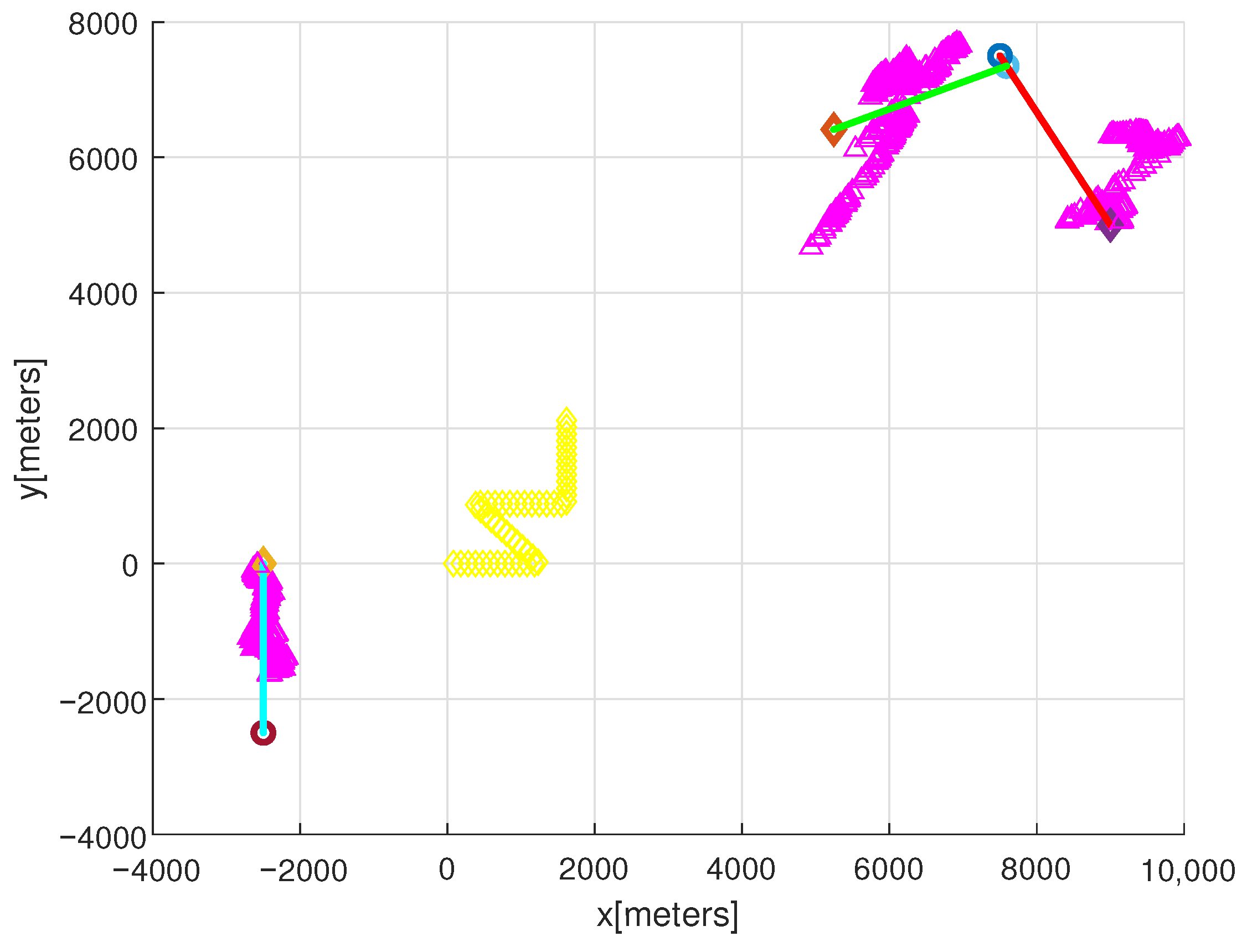
See Figure 1 for the simulation scenario. In this figure, the observer’s path is marked with yellow colors. Every target moves with a constant velocity. In Figure 1, we present the direction of target motion using symbols. A circle symbol indicates the start point of a target motion and a diamond symbol indicates the end point of a target motion.

Figure 1.
For clear presentation of the observer’s path, this figure simulates the case where there is no interference point. The observer’s path is marked with yellow colors. Target 1 (red) starts from [7500, 7500] and moves with velocity [3, −5] in m/s. Target 2 (blue) starts from [−2500, −2500] and moves with velocity [0, 5] in m/s. Targets 1 (red) and 2 (blue) are generated at sampling-stamp 0, and target 3 (green) is spawned from target 1 at 30 s. Target 3 (green) moves with velocity [−5, −2] in m/s. We present the direction of target motion using symbols. A circle symbol indicates the start point of a target motion, and a diamond symbol indicates the end point of a target motion. The estimated target position is marked with magenta triangles.
Since the sonar’s maximum sensing range is 10 km, we deploy a target initially so that it can be detected by the observer. The position of each target at every second is marked with distinct colors. Target 1 (red) starts from [7500, 7500] and moves with velocity [3, −5] in m/s. Target 2 (blue) starts from [−2500, −2500] and moves with velocity [0, 5] in m/s. Targets 1 (red) and 2 (blue) are generated at sampling-stamp 0, and target 3 (green) is spawned from target 1 at 30 s. Target 3 (green) moves with velocity [−5, −2] in m/s.
For clear presentation of the observer’s path, Figure 1 simulates the case where there is no interference point. In other words, Figure 1 shows the simulation result without interference points. In this figure, the estimated target position is marked with magenta triangles. Before the observer maneuver at 125 s, true target positions are not tracked by target estimations (magenta triangles). However, as time goes on, true target positions are tracked by target estimations.
Considering the simulation of the scenario in Figure 1, Figure 2 shows the simulation result with interference points. Recall that (16) is the average number of interference points at sampling-stamp k. We set , which implies that, on average, one interference point is generated at each sampling-stamp. In Figure 2, the estimated target position is marked with magenta triangles. Due to interference points, many false targets are generated surrounding the observer. Before the observer maneuver at 125 s, true target positions are not tracked by target estimations (magenta triangles). However, as time goes on, true target positions are tracked by target estimations.
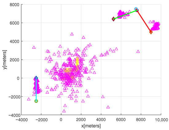
Figure 2.
This figure shows the simulation result with interference points. We set , which implies that, on average, one interference point is generated at each sampling-stamp. The estimated target position is marked with magenta triangles. Before the observer maneuver at 125 s, true target positions are not tracked by target estimations (magenta triangles). However, as time goes on, true target positions are tracked by target estimations.
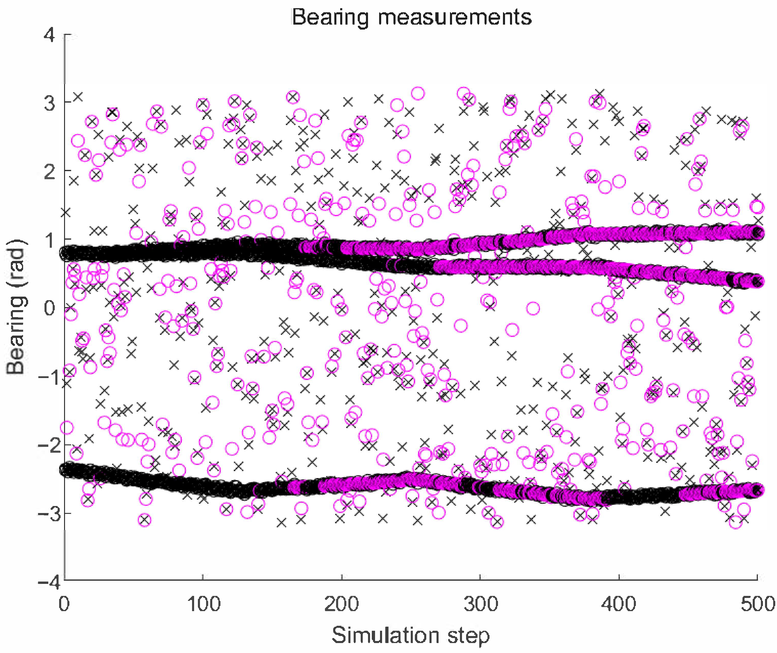
Considering the simulation of Figure 2, Figure 3 shows the bearing (in radians) change with respect to time (in seconds). In this figure, true target bearing measurements are marked with circles. In addition, interference points are marked with crosses. The estimated target bearing is marked with magenta circles. Before the observer maneuver at 125 s, true target bearings are not tracked by the estimated target bearing (magenta circles). However, as time goes on, true target bearings are tracked by estimated target bearings.
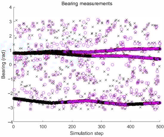
Figure 3.
The bearing (in radians) change with respect to time (in seconds). In this figure, true target bearings are marked with circles. In addition, interference points are marked with crosses. The estimated target bearing is marked with magenta circles. Before the observer maneuver at 125 s, true target bearings are not tracked by the estimated target bearing (magenta circles). However, as time goes on, true target bearings are tracked by estimated target bearings.
4.1. Monte-Carlo (MC) Simulations
A total of 100 Monte-Carlo (MC) simulations are utilized for verifying the outperformance of the proposed filter. Let denote the number of total MC simulations. We set , which implies that, on average, one interference point is generated at each sampling-stamp. We generate target samples using every bearing measurement at every sampling-stamp. It takes 14 s to run a single MC simulation.
Tracking accuracy is checked with the cardinality (number of targets) and the Optimal Subpattern Assignment (OSPA) metric [31,32]. We derive the cardinality as the mean of the estimated number of targets under MC simulations. We also derive the mean of OSPA using MC simulations.
Recall that in (28) is the number of components of the intensity. The cardinality at sampling-stamp k is defined as
The true cardinality at sampling-stamp k indicates the true number of targets detected at sampling-stamp k.
We briefly address the Optimal Subpattern Assignment (OSPA) metric in [31,32]. Let denote the distance between and . Here, c denotes a cut-off parameter in [31,32]. In our simulations, we use .
Let denote the set of target position estimates at sample-step k. Recall that denotes the number of components of the intensity. Suppose that there are targets at sample-step k. Let denote the true target positions at sample-step k. The OSPA distance between the target estimates and the true target positions is defined as
Here, denotes the set of permutations on . The OSPA metric can be computed efficiently by using the Hungarian method for optimal point assignment [31,32].
The mean of OSPA at sample-step k is
See Figure 4 for the OSPA and the cardinality of the proposed GM-PHD. Before 30 s pass, there are two targets (Targets 1 and 2). Target 3 is spawned from target 1 at 30 s. In bearing-only target tracking, observer maneuver is required for target localization [27,28]. The observer maneuvers at 125 s. See that the OSPA decreases gradually after the observer maneuver. In Figure 4, plots the number of bearing measurements associated with true targets. In addition, is the mean of the estimated number of targets using 100 MC simulations. As time goes on, OSPA gradually approaches to zero and converges to in cardinality. In other words, the cardinality error converges to almost zero as time goes on.
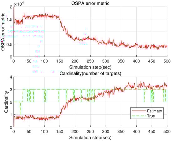
Figure 4.
The OSPA and the cardinality of the proposed GM-PHD in the case where is utilized. As time goes on, OSPA gradually approaches to zero and converges to in cardinality.
4.1.1. Comparison with the Case Where a Single EKF Is Used in the GM-PHD
Note that the nonlinearity of the bearing-only measurements can be handled by the EKF when applying the GM-PHD filter. However, range uncertainty of the target is large for bearing-only measurements ( km in MATLAB simulations). This results in poor performance when a single EKF is used in the GM-PHD. Setting corresponds to the case where we apply a single EKF in the GM-PHD. As we increase B, we distribute more target samples considering the maximum sensing range of the bearing sensor. Consider the scenario in Figure 2. We next check the effect of changing B, the number of target samples generated using every bearing measurement at every sampling-stamp.
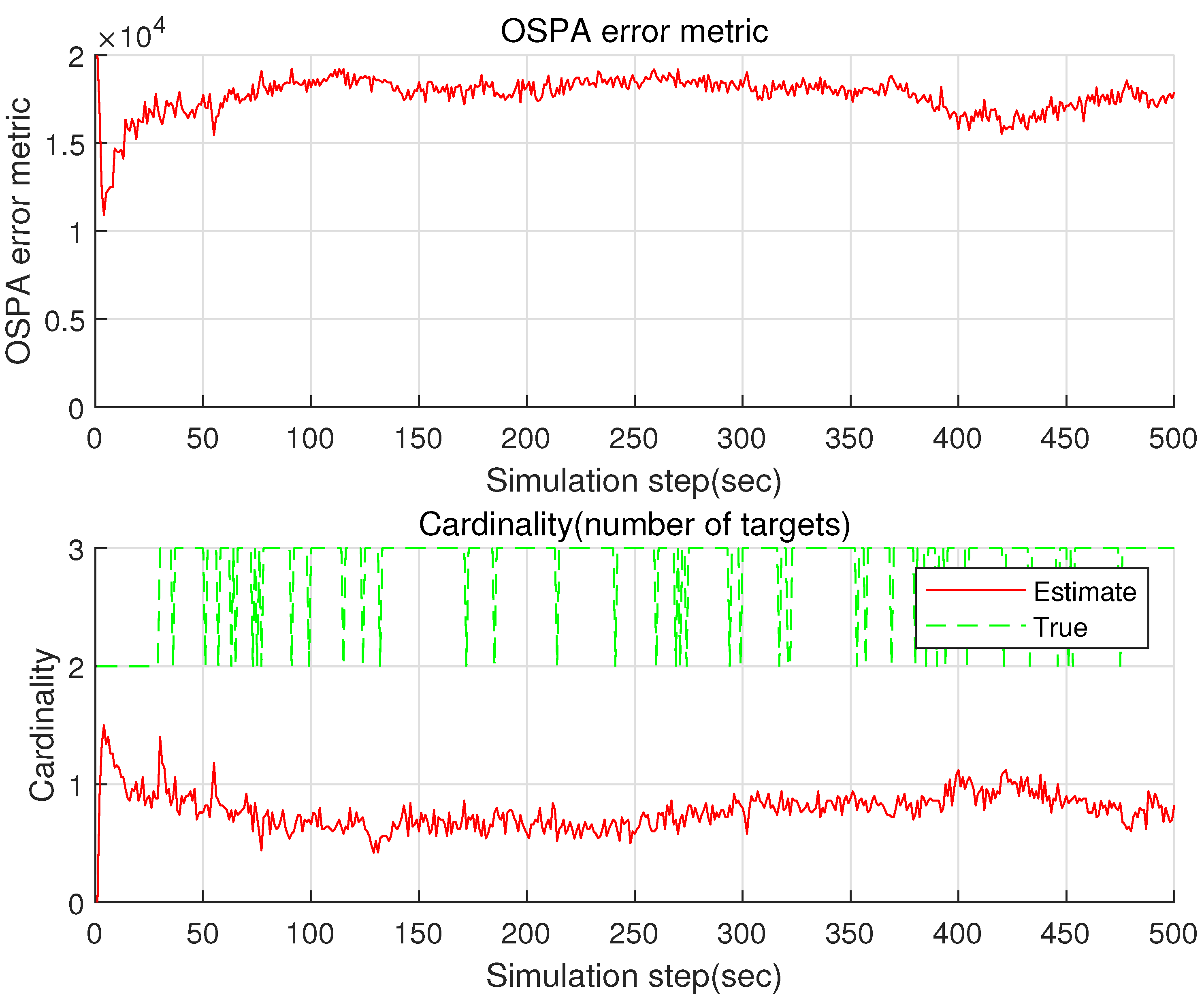
Considering the case where is utilized, Figure 5 plots the OSPA and the cardinality of the proposed GM-PHD. Compared with the case where is used (Figure 4), the estimation accuracy decreases considerably. This shows the effectiveness of the proposed sample distribution approach used in our paper. It takes 6 s to run a single MC simulation, as we utilize . Compared with the case where is used (Figure 4), the computational load decreases.
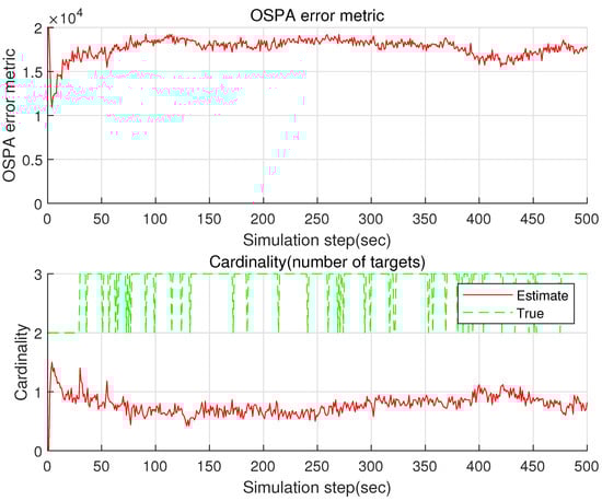
Figure 5.
The OSPA and the cardinality of the proposed GM-PHD in the case where is utilized. Setting corresponds to the case where we apply a single EKF in the GM-PHD. Compared with the case where is used (Figure 4), the estimation accuracy decreases considerably.
4.1.2. The Effect of Changing B
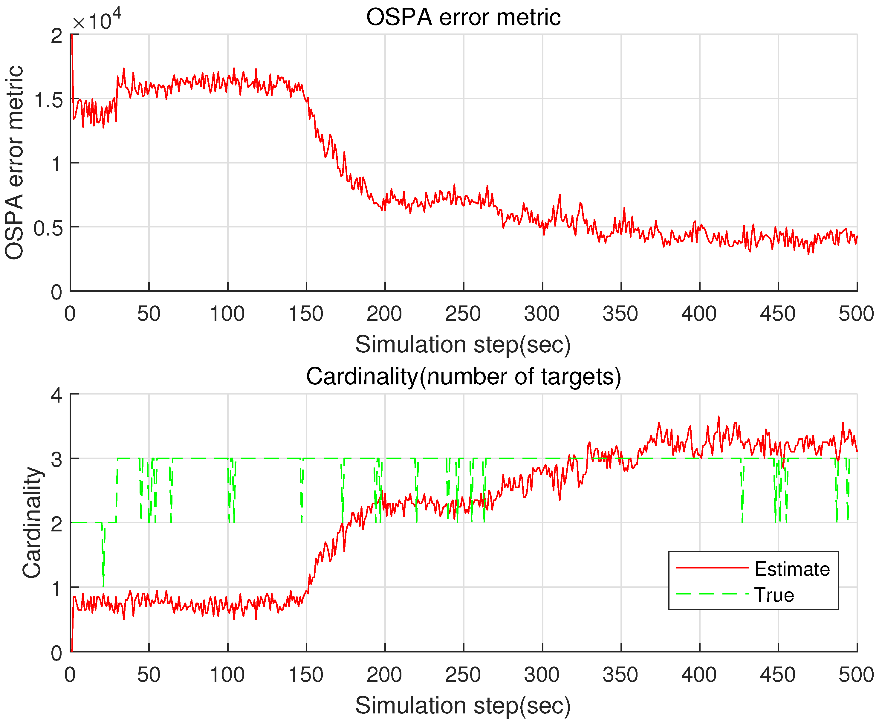
Considering the case where is utilized, Figure 6 plots the OSPA and the cardinality of the proposed GM-PHD. Compared with the case where is used (Figure 5), the estimation accuracy increases considerably. It takes 6 s to run a single MC simulation. Compared with the case where is used, the computational load decreases.
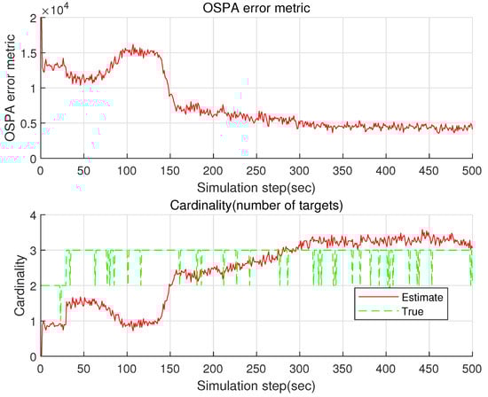
Figure 6.
The OSPA and the cardinality of the proposed GM-PHD in the case where is utilized.
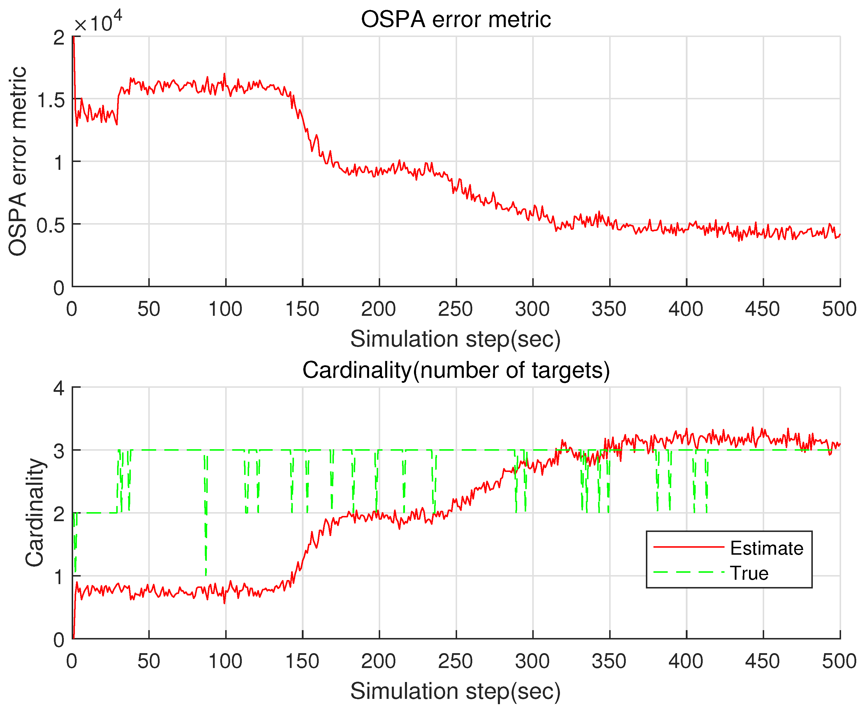
Considering the case where is utilized, Figure 7 plots the OSPA and the cardinality of the proposed GM-PHD. Compared with the case where is used (Figure 5), the estimation accuracy increases considerably. It takes 7 s to run a single MC simulation. Compared with the case where is used, the computational load decreases.
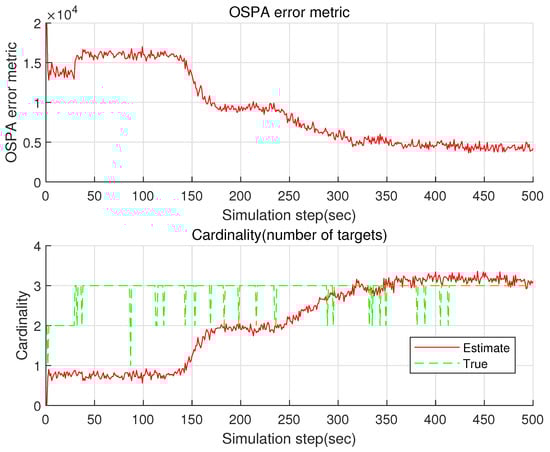
Figure 7.
The OSPA and the cardinality of the proposed GM-PHD in the case where is utilized.
Table 1 shows the computational load (running time for one MC simulation) as B varies. Recall that setting corresponds to the case where we apply a single EKF in the GM-PHD. Table 1 shows that as B increases, the computational load increases in general. However, considering both the computational load and the estimation accuracy (Figure 6), setting is desirable.

Table 1.
Computational load analysis.
5. Conclusions
This article handles tracking multiple targets using bearing-only measurements in underwater noisy environments. We apply GM-PHD filters to solve our MTT problem based on bearing-only measurements. Since bearing-only measurements do not provide position information of a target, we make every bearing measurement give birth to B target samples, which are distributed considering the feasible range of the passive sensor. The effectiveness of the proposed GM-PHD is verified utilizing MATLAB simulations.
In the future, we will extend the proposed tracking filter so that one can handle the case where multiple observers are used for tracking multiple targets in noisy environments under bearing-only measurements. As we use multiple observers, false targets may appear as bearing lines of multiple observers’ intersects. Thus, we require filters for removing false targets effectively.
Funding
This research received no external funding.
Institutional Review Board Statement
Not applicable.
Informed Consent Statement
Not applicable.
Data Availability Statement
Not applicable.
Conflicts of Interest
The authors declare no conflict of interest.
References
- Luo, W.; Xing, J.; Milan, A.; Zhang, X.; Liu, W.; Kim, T.K. Multiple object tracking: A literature review. Artif. Intell. 2021, 293, 103448. [Google Scholar] [CrossRef]
- Ozer, E.; Akar, A.O.; Hocaoglu, A.K. Passive sonar multiple target tracking with different resampling algorithms. In Proceedings of the 2018 26th Signal Processing and Communications Applications Conference (SIU), Izmir, Turkey, 2–5 May 2018; pp. 1–4. [Google Scholar]
- Sheng, X.; Chen, Y.; Guo, L.; Yin, J.; Han, X. Multitarget Tracking Algorithm Using Multiple GMPHD Filter Data Fusion for Sonar Networks. Sensors 2018, 18, 3193. [Google Scholar] [CrossRef] [PubMed] [Green Version]
- Mohanna, M.; Rabeh, M.L.; Zieur, E.M.; Hekala, S. Optimization of MUSIC algorithm for angle of arrival estimation in wireless communications. NRIAG J. Astron. Geophys. 2013, 2, 116–124. [Google Scholar] [CrossRef] [Green Version]
- Qian, C.; Huang, L.; So, H. Computationally efficient ESPRIT algorithm for direction-of-arrival estimation based on Nyström method. Signal Process. 2014, 94, 74–80. [Google Scholar] [CrossRef]
- Gupta, P.; Kar, S. MUSIC and improved MUSIC algorithm to estimate direction of arrival. In Proceedings of the 2015 International Conference on Communications and Signal Processing (ICCSP), Melmaruvathur, India, 2–4 April 2015; pp. 0757–0761. [Google Scholar]
- Kim, J. Direction of Arrival Estimation Using Four Isotropic Receivers. IEEE Instrum. Meas. Mag. 2021, 24, 77–81. [Google Scholar] [CrossRef]
- Wen, F.; Javed, U.; Yang, Y.; He, D.; Zhang, Y. Improved subspace direction-of-arrival estimation in unknown nonuniform noise fields. In Proceedings of the 2016 Fourth International Conference on Ubiquitous Positioning, Indoor Navigation and Location Based Services (UPINLBS), Shanghai, China, 2–4 November 2016; pp. 230–233. [Google Scholar]
- Kim, J. Obstacle Information Aided Target Tracking Algorithms for Angle-Only Tracking of a Highly Maneuverable Target in Three Dimensions. IET Radar Sonar Navig. 2019, 13, 1074–1080. [Google Scholar] [CrossRef]
- Kim, J. Observer manoeuvre control to track multiple targets considering Doppler-bearing measurements in threat environments. IET Radar Sonar Navig. 2019, 13, 2158–2165. [Google Scholar] [CrossRef]
- Kim, J. Maneuvering target tracking of underwater autonomous vehicles based on bearing-only measurements assisted by inequality constraints. Ocean Eng. 2019, 189, 106404. [Google Scholar] [CrossRef]
- Nardone, S.; Lindgren, A.; Gong, K. Fundamental properties and performance of conventional bearings-only target motion analysis. IEEE Trans. Autom. Control 1984, 29, 775–787. [Google Scholar] [CrossRef]
- Clark, J.; Vinter, R.; Yaqoob, M. The shifted Rayleigh filter for bearings only tracking. In Proceedings of the 2005 7th International Conference on Information Fusion, Philadelphia, PA, USA, 25–28 July 2005; Volume 1, p. 8. [Google Scholar]
- Kim, J.; Suh, T.; Ryu, J. Bearings-only target motion analysis of a highly manoeuvring target. IET Radar Sonar Navig. 2017, 11, 1011–1019. [Google Scholar] [CrossRef]
- Jiang, H.; Cai, Y. Bearings-only tracking with a Gaussian-sum based ensemble Kalman filter. In Proceedings of the 2017 29th Chinese Control And Decision Conference (CCDC), Chongqing, China, 28–30 May 2017; pp. 4823–4828. [Google Scholar]
- Li, L.; Xie, W.; Liu, Z. Bearings-only maneuvering target tracking based on truncated quadrature Kalman filtering. Int. J. Electron. Commun. 2015, 69, 281–289. [Google Scholar]
- Ristic, B.; Houssineau, J.; Arulampalam, S. Robust target motion analysis using the possibility particle filter. IET Radar Sonar Navig. 2019, 13, 18–22. [Google Scholar] [CrossRef]
- Ristic, B.; Arulampalam, S.; Gordon, N. Beyond the Kalman Filter: Particle Filters for Tracking Applications; Artech House: Norwood, MA, USA, 2004. [Google Scholar]
- Peach, N. Bearings-only tracking using a set of range-parameterised extended Kalman filters. IEE Proc. Control Theory Appl. 1995, 142, 73–80. [Google Scholar] [CrossRef]
- Karlsson, R.; Gustafsson, F. Recursive Bayesian estimation: Bearing-only applications. IEE Proc. Radar Sonar Navig. 2005, 152, 305–313. [Google Scholar] [CrossRef] [Green Version]
- Blackman, S. Multiple hypothesis tracking for multiple target tracking. IEEE Aerosp. Electron. Syst. Mag. 2004, 19, 5–18. [Google Scholar] [CrossRef]
- He, S.; Shin, H.S.; Tsourdos, A. Joint Probabilistic Data Association Filter with Unknown Detection Probability and Clutter Rate. Sensors 2018, 18, 269. [Google Scholar] [CrossRef] [Green Version]
- Musicki, D.; Kaune, R.; Koch, W. Mobile Emitter Geolocation and Tracking Using TDOA and FDOA Measurements. IEEE Trans. Signal Process. 2009, 58, 1863–1874. [Google Scholar] [CrossRef]
- Vo, B.N.; Singh, S.; Doucet, A. Sequential Monte Carlo methods for multitarget filtering with random finite sets. IEEE Trans. Aerosp. Electron. Syst. 2005, 41, 1224–1245. [Google Scholar]
- Vo, B.N.; Ma, W.K. The Gaussian Mixture Probability Hypothesis Density Filter. IEEE Trans. Signal Process. 2006, 54, 4091–4104. [Google Scholar] [CrossRef]
- Wang, X.; Han, C. An improved multiple model GM-PHD filter for maneuvering target tracking. Chin. J. Aeronaut. 2013, 26, 179–185. [Google Scholar] [CrossRef] [Green Version]
- Oshman, Y.; Davidson, P. Optimization of observer trajectories for bearings-only target localization. IEEE Trans. Aerosp. Electron. Syst. 1999, 35, 892–902. [Google Scholar] [CrossRef]
- Baek, S.S.; Kwon, H.; Yoder, J.A.; Pack, D. Optimal Path Planning of a Target-Following Fixed-Wing UAV Using Sequential Decision Processes. In Proceedings of the Proceedings of the IEEE/RSJ International Conference on Intelligent Robots and Systems (IROS), Tokyo, Japan, 3–7 November 2013; pp. 2959–2962.
- Mahler, R. Multitarget Bayes filtering via first-order multitarget moments. IEEE Trans. Aerosp. Electron. Syst. 2003, 39, 1152–1178. [Google Scholar] [CrossRef]
- Gao, Y.; Jiang, D.; Zhang, C.; Guo, S. A Labeled GM-PHD Filter for Explicitly Tracking Multiple Targets. Sensors 2021, 21, 3932. [Google Scholar] [CrossRef] [PubMed]
- Schuhmacher, D.; Vo, B.T.; Vo, B.N. A Consistent Metric for Performance Evaluation of Multi-Object Filters. IEEE Trans. Signal Process. 2008, 56, 3447–3457. [Google Scholar] [CrossRef] [Green Version]
- Nguyen, H.V.; Rezatofighi, H.; Vo, B.N.; Ranasinghe, D.C. Distributed Multi-Object Tracking Under Limited Field of View Sensors. IEEE Trans. Signal Process. 2021, 69, 5329–5344. [Google Scholar] [CrossRef]


Publisher’s Note: MDPI stays neutral with regard to jurisdictional claims in published maps and institutional affiliations. |
© 2022 by the author. Licensee MDPI, Basel, Switzerland. This article is an open access article distributed under the terms and conditions of the Creative Commons Attribution (CC BY) license (https://creativecommons.org/licenses/by/4.0/).