
BO-ALLCNN: Bayesian-Based Optimized CNN for Acute Lymphoblastic Leukemia Detection in Microscopic Blood Smear Images


Abstract
:1. Introduction
- Development of a new optimized deep learning CNN for the detection of ALL in microscopic blood smear images.
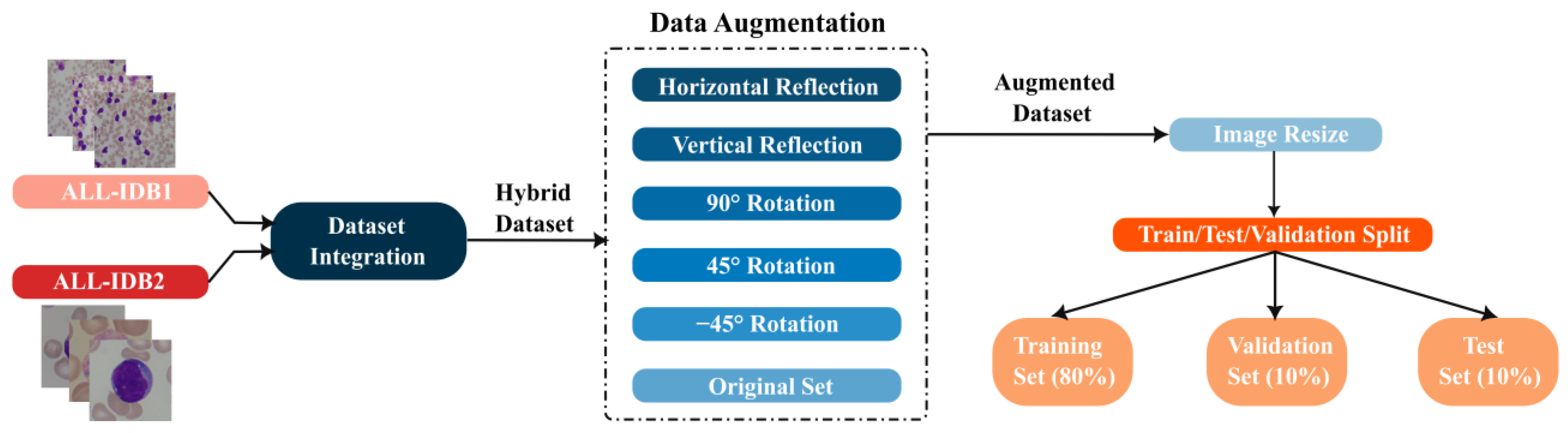
- Formation of a hybrid dataset by integrating two public ALL datasets to supplement the input data.
- Augmentation of the hybrid dataset using several image transformations to promote classification performance.
- Determination of the optimal architecture and hyperparameters of the proposed CNN using the Bayesian optimization approach.
- Comparison between the optimized model and a non-optimized model to investigate the effectiveness of Bayesian optimization in improving classification performance.
- Classification performance comparison of the optimal ALL CNN model with that of the state of the art.
2. Literature Review
3. Materials and Methods
3.1. Datasets
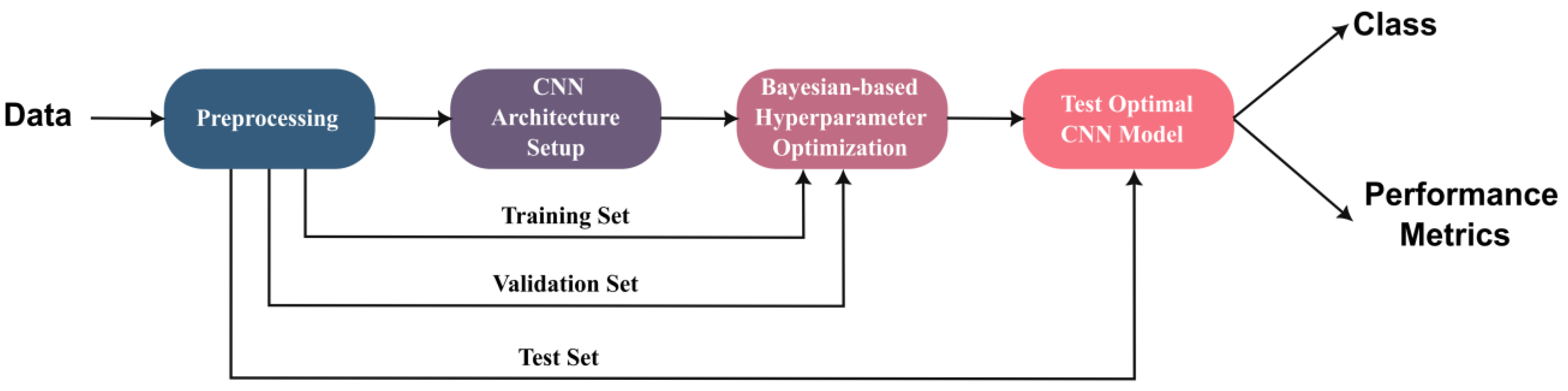
3.2. Proposed Framework
3.2.1. Data Preprocessing
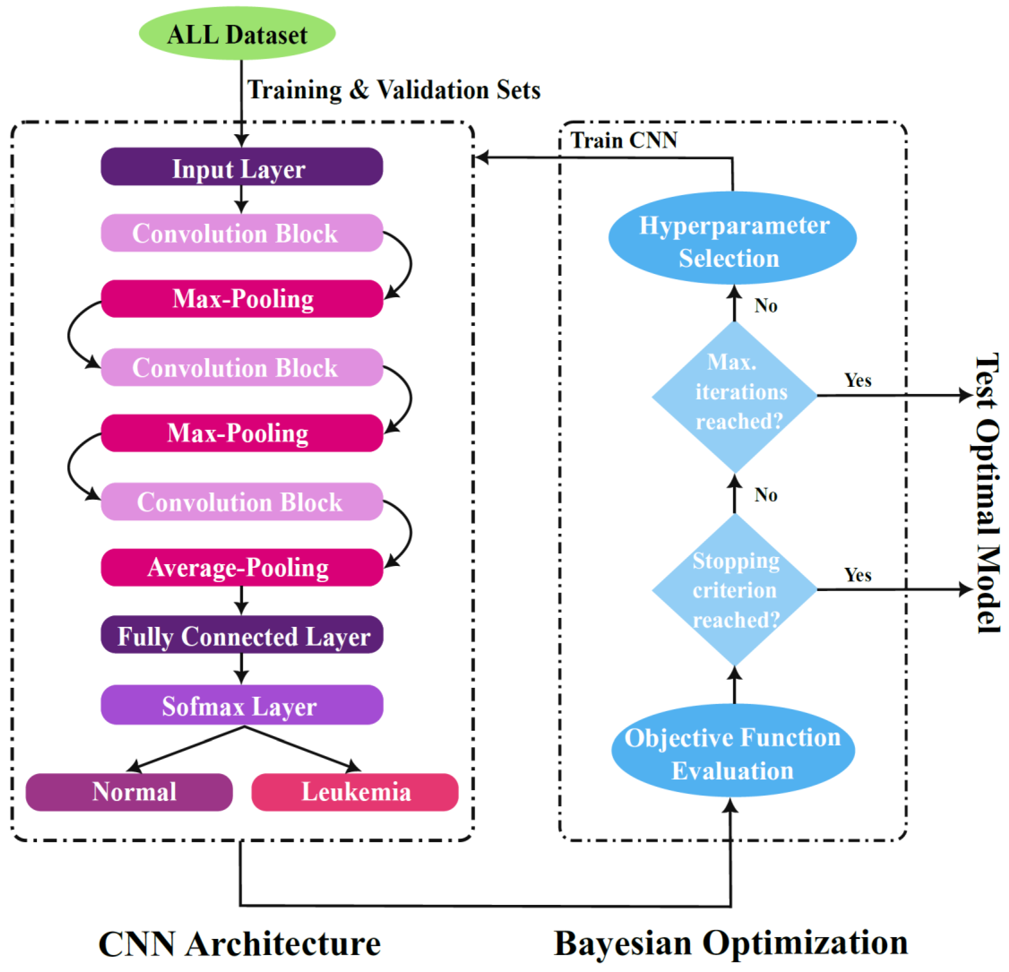
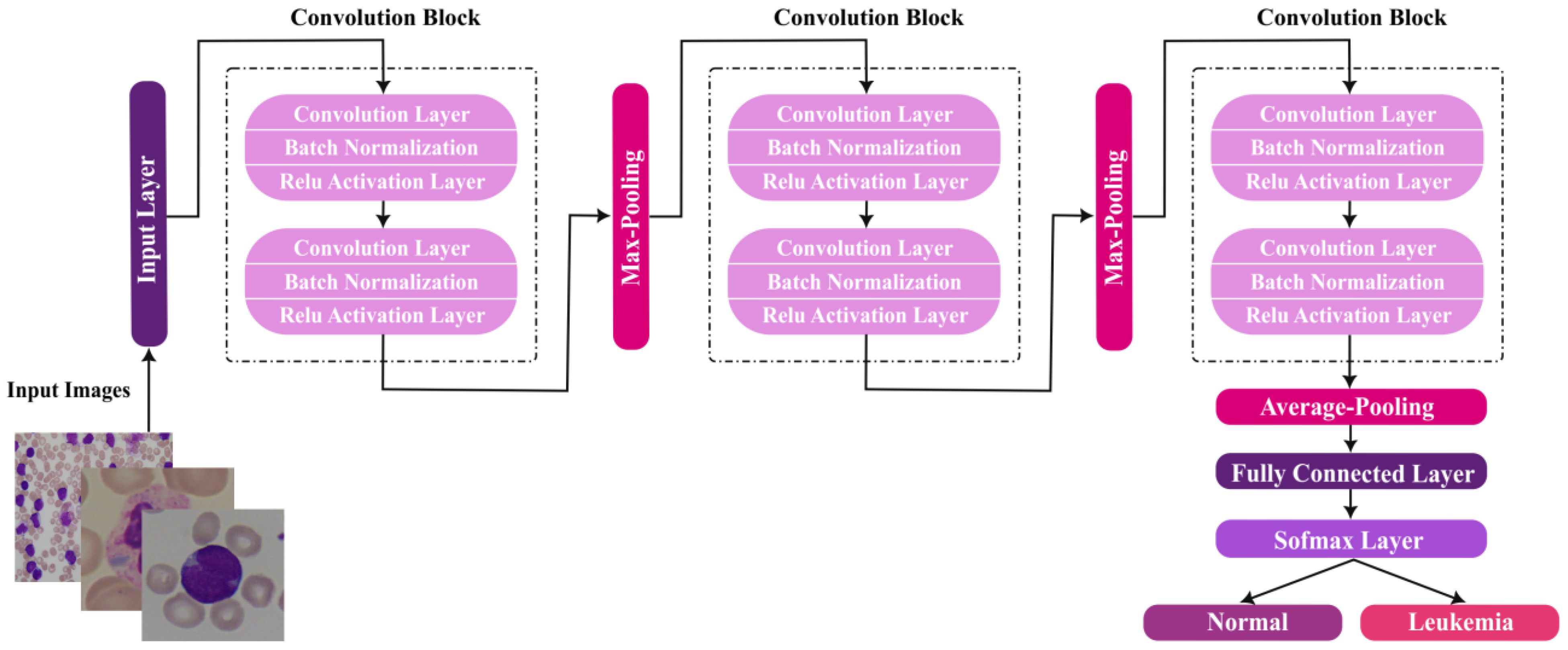
3.2.2. Proposed CNN Architecture Setup
3.2.3. Hyperparameter Optimization
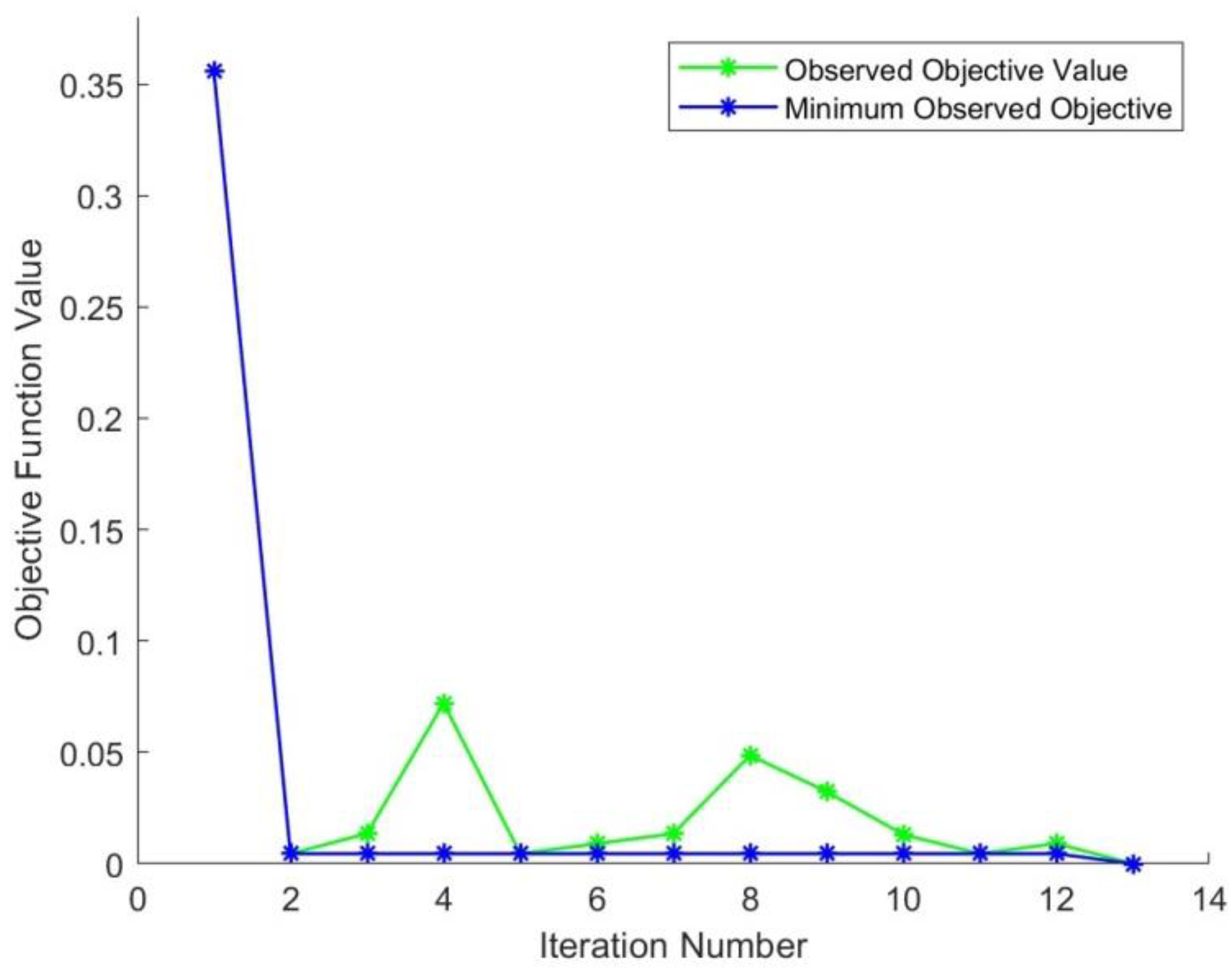
Bayesian Optimization Algorithm
Optimization Variables
- Initial Learning Rate
- 2.
- Convolutional Block Depth (CBD)
- 3.
- Stochastic Gradient Descent Momentum
- 1.
- Regularization Coefficient
3.2.4. Optimal Model Selection and Testing
4. Results
5. Conclusions
Author Contributions
Funding
Institutional Review Board Statement
Informed Consent Statement
Data Availability Statement
Acknowledgments
Conflicts of Interest
References
- Common Cancer Types—NCI. Available online: https://www.cancer.gov/types/common-cancers (accessed on 1 July 2022).
- Leukemia—Cancer Stat Facts. Available online: https://seer.cancer.gov/statfacts/html/leuks.html (accessed on 30 June 2022).
- Emadi, A.; Karp, J.E. Acute Leukemia: An Illustrated Guide to Diagnosis and Treatment. Angew. Chem. Int. Ed. 2018, 6, 951–952. [Google Scholar]
- Ghaderzadeh, M.; Asadi, F.; Hosseini, A.; Bashash, D.; Abolghasemi, H.; Roshanpour, A. Machine Learning in Detection and Classification of Leukemia Using Smear Blood Images: A Systematic Review. Sci. Program. 2021, 2021, 9933481. [Google Scholar] [CrossRef]
- Sajjad, M.; Khan, S.; Jan, Z.; Muhammad, K.; Moon, H.; Kwak, J.T.; Rho, S.; Baik, S.W.; Mehmood, I. Leukocytes Classification and Segmentation in Microscopic Blood Smear: A Resource-Aware Healthcare Service in Smart Cities. IEEE Access 2017, 5, 3475–3489. [Google Scholar] [CrossRef]
- Thanh, T.T.P.; Vununu, C.; Atoev, S.; Lee, S.-H.; Kwon, K.-R. Leukemia Blood Cell Image Classification Using Convolutional Neural Network. Int. J. Comput. Theory Eng. 2018, 10, 54–58. [Google Scholar] [CrossRef]
- Loey, M.; Naman, M.; Zayed, H. Deep Transfer Learning in Diagnosing Leukemia in Blood Cells. Computers 2020, 9, 29. [Google Scholar] [CrossRef]
- Vogado, L.H.S.; Veras, R.M.S.; Araujo, F.H.D.; Silva, R.R.V.; Aires, K.R.T. Leukemia diagnosis in blood slides using transfer learning in CNNs and SVM for classification. Eng. Appl. Artif. Intell. 2018, 72, 415–422. [Google Scholar] [CrossRef]
- Esteva, A.; Chou, K.; Yeung, S.; Naik, N.; Madani, A.; Mottaghi, A.; Liu, Y.; Topol, E.; Dean, J.; Socher, R. Deep learning-enabled medical computer vision. Npj Digit. Med. 2021, 4, 5. [Google Scholar] [CrossRef]
- Bibi, N.; Sikandar, M.; Din, I.U.; Almogren, A.; Ali, S. IOMT-based automated detection and classification of leukemia using deep learning. J. Healthc. Eng. 2020, 2020, 6648574. [Google Scholar] [CrossRef]
- Suriyasekeran, K.; Santhanamahalingam, S.; Duraisamy, M. Algorithms for Diagnosis of Diabetic Retinopathy and Diabetic Macula Edema—A Review. Adv. Exp. Med. Biol. 2021, 1307, 357–373. [Google Scholar] [CrossRef]
- Zhao, W.; Jiang, W.; Qiu, X. Deep learning for COVID-19 detection based on CT images. Sci. Rep. 2021, 11, 1–12. [Google Scholar] [CrossRef]
- Atteia, G.E.; Mengash, H.A.; Samee, N.A. Evaluation of using Parametric and Non-parametric Machine Learning Algorithms for COVID-19 Forecasting. Int. J. Adv. Comput. Sci. Appl. 2021, 12, 647–657. [Google Scholar] [CrossRef]
- Sheikh, A.; McMenamin, J.; Taylor, B.; Robertson, C. SARS-CoV-2 Delta VOC in Scotland: Demographics, risk of hospital admission, and vaccine effectiveness. Lancet 2021, 397, 2461–2462. [Google Scholar] [CrossRef]
- Deng, Z.; Wang, Z.; Tang, Z.; Huang, K.; Zhu, H. A deep transfer learning method based on stacked autoencoder for cross-domain fault diagnosis. Appl. Math. Comput. 2021, 408, 126318. [Google Scholar] [CrossRef]
- Lecun, Y.; Bengio, Y.; Hinton, G. Deep learning. Nature 2015, 521, 436–444. [Google Scholar] [CrossRef]
- Khan, U.; Khan, S.; Rizwan, A.; Atteia, G.; Jamjoom, M.M.; Samee, N.A. Aggression Detection in Social Media from Textual Data Using Deep Learning Models. Appl. Sci. 2022, 12, 5083. [Google Scholar] [CrossRef]
- Samee, N.A.; Atteia, G.; Alkanhel, R.; Alhussan, A.A.; Aleisa, H.N. Hybrid Feature Reduction Using PCC-Stacked Autoencoders for Gold/Oil Prices Forecasting under COVID-19 Pandemic. Electronics 2022, 11, 991. [Google Scholar] [CrossRef]
- Yamashita, R.; Nishio, M.; Do, R.K.G.; Togashi, K. Convolutional neural networks: An overview and application in radiology. Insights Imaging 2018, 9, 611–629. [Google Scholar] [CrossRef]
- Eckardt, J.N.; Middeke, J.M.; Riechert, S.; Schmittmann, T.; Sulaiman, A.S.; Kramer, M.; Sockel, K.; Kroschinsky, F.; Schuler, U.; Schetelig, J.; et al. Deep learning detects acute myeloid leukemia and predicts NPM1 mutation status from bone marrow smears. Leukemia 2021, 36, 111–118. [Google Scholar] [CrossRef]
- Atteia, G.; Samee, N.A.; Hassan, H.Z. DFTSA-Net: Deep Feature Transfer-Based Stacked Autoencoder Network for DME Diagnosis. Entropy 2021, 23, 1251. [Google Scholar] [CrossRef]
- Alagu, S.; Priyanka, A.N.; Kavitha, G.; Bagan, B.K. Automatic Detection of Acute Lymphoblastic Leukemia Using UNET Based Segmentation and Statistical Analysis of Fused Deep Features. Appl. Artif. Intell. 2021, 35, 1952–1969. [Google Scholar] [CrossRef]
- Samee, N.A.; Alhussan, A.A.; Ghoneim, V.F.; Atteia, G.; Alkanhel, R.; Al-antari, M.A.; Kadah, Y.M. A Hybrid Deep Transfer Learning of CNN-Based LR-PCA for Breast Lesion Diagnosis via Medical Breast Mammograms. Sensors 2022, 22, 4938. [Google Scholar] [CrossRef] [PubMed]
- Fan, H.; Zhang, F.; Xi, L.; Li, Z.; Liu, G.; Xu, Y. LeukocyteMask: An automated localization and segmentation method for leukocyte in blood smear images using deep neural networks. J. Biophotonics 2019, 12, e201800488. [Google Scholar] [CrossRef] [PubMed]
- Prangemeier, T.; Reich, C.; Koeppl, H. Attention-Based Transformers for Instance Segmentation of Cells in Microstructures. In Proceedings of the 2020 IEEE International Conference on Bioinformatics and Biomedicine (BIBM), Seoul, Korea, 16–19 December 2020; pp. 700–707. [Google Scholar] [CrossRef]
- Wu, Y.; Ge, Z.; Zhang, D.; Xu, M.; Zhang, L.; Xia, Y.; Cai, J. Enforcing Mutual Consistency of Hard Regions for Semi-supervised Medical Image Segmentation. Arvix 2021, 4. [Google Scholar] [CrossRef]
- Zhang, D.; Song, Y.; Liu, D.; Jia, H.; Liu, S.; Xia, Y.; Huang, H.; Cai, W. Panoptic segmentation with an end-to-end cell R-CNN for pathology image analysis. Lect. Notes Comput. Sci. 2018, 11071 LNCS, 237–244. [Google Scholar] [CrossRef]
- Liu, W.; Li, C.; Xu, N.; Jiang, T.; Rahaman, M.M.; Sun, H.; Wu, X.; Hu, W.; Chen, H.; Sun, C.; et al. CVM-Cervix: A hybrid cervical Pap-smear image classification framework using CNN, visual transformer and multilayer perceptron. Pattern Recognit. 2022, 130, 108829. [Google Scholar] [CrossRef]
- Song, Y.; Chang, H.; Gao, Y.; Liu, S.; Zhang, D.; Yao, J.; Chrzanowski, W.; Cai, W. Feature learning with component selective encoding for histopathology image classification. Proc. Int. Symp. Biomed. Imaging 2018, 2018, 257–260. [Google Scholar] [CrossRef]
- Ouyang, N.; Wang, W.; Ma, L.; Wang, Y.; Chen, Q.; Yang, S.; Xie, J.; Su, S.; Cheng, Y.; Cheng, Q.; et al. Diagnosing acute promyelocytic leukemia by using convolutional neural network. Clin. Chim. Acta. 2021, 512, 1–6. [Google Scholar] [CrossRef]
- Liu, D.; Zhang, D.; Song, Y.; Zhang, F.; O’Donnell, L.; Huang, H.; Chen, M.; Cai, W. Unsupervised Instance Segmentation in Microscopy Images via Panoptic Domain Adaptation and Task Re-weighting. Proc. IEEE Comput. Soc. Conf. Comput. Vis. Pattern Recognit. 2020, 4242–4251. [Google Scholar] [CrossRef]
- Tang, F.; Wang, X.; Ran, A.R.; Chan, C.; Ho, M.; Yip, W.; Young, A.; Lok, J.; Szeto, S.; Chan, J.; et al. A Multitask Deep-Learning System to Classify Diabetic Macular Edema for Different Optical Coherence Tomography Devices: A Multicenter Analysis. Diabetes Care 2021, 44, 2078–2088. [Google Scholar] [CrossRef]
- Goodfellow, I.; Bengio, Y.; Courville, A. Deep Learning—Adaptive Computation and Machine Learning; The MIT Press: Cambridge, MA, USA, 2017; Volume 1, ISBN 978-0-262-03561-3. [Google Scholar]
- Hutter, F.; Kotthoff, L.; Vanschoren, J. Automated Machine Learning; Hutter, F., Kotthoff, L., Vanschoren, J., Eds.; The Springer Series on Challenges in Machine Learning; Springer International Publishing: Berlin, Germany, 2019; ISBN 978-3-030-05317-8. [Google Scholar]
- Negm, A.S.; Hassan, O.A.; Kandil, A.H. A decision support system for Acute Leukaemia classification based on digital microscopic images. Alex. Eng. J. 2018, 57, 2319–2332. [Google Scholar] [CrossRef]
- Begum, A.R.J.; Razak, D.T.A. A Proposed Novel Method for Detection and Classification of Leukemia using Blood Microscopic Images. Int. J. Adv. Res. Comput. Sci. 2017, 8, 147–151. [Google Scholar] [CrossRef]
- Jothi, G.; Inbarani, H.H.; Azar, A.T.; Devi, K.R. Rough set theory with Jaya optimization for acute lymphoblastic leukemia classification. Neural Comput. Appl. 2019, 31, 5175–5194. [Google Scholar] [CrossRef]
- Agaian, S.; Madhukar, M.; Chronopoulos, A.T. Automated screening system for acute myelogenous leukemia detection in blood microscopic images. IEEE Syst. J. 2014, 8, 995–1004. [Google Scholar] [CrossRef]
- Kazemi, F.; Najafabadi, T.; Araabi, B. Automatic Recognition of Acute Myelogenous Leukemia in Blood Microscopic Images Using K-means Clustering and Support Vector Machine. J. Med. Signals Sens. 2016, 6, 183. [Google Scholar] [CrossRef] [PubMed]
- Amin, M.M.; Kermani, S.; Talebi, A.; Oghli, M.G. Recognition of acute lymphoblastic leukemia cells in microscopic images using k-means clustering and support vector machine classifier. J. Med. Signals Sens. 2015, 5, 49. [Google Scholar] [CrossRef]
- Muthumayil, K.; Manikandan, S.; Srinivasan, S.; Escorcia-Gutierrez, J.; Gamarra, M.; Mansour, R.F. Diagnosis of leukemia disease based on enhanced virtual neural network. Comput. Mater. Contin. 2021, 69, 2031–2044. [Google Scholar] [CrossRef]
- Al-jaboriy, S.S.; Sjarif, N.N.A.; Chuprat, S.; Abduallah, W.M. Acute lymphoblastic leukemia segmentation using local pixel information. Pattern Recognit. Lett. 2019, 125, 85–90. [Google Scholar] [CrossRef]
- Bodzas, A.; Kodytek, P.; Zidek, J. Automated Detection of Acute Lymphoblastic Leukemia From Microscopic Images Based on Human Visual Perception. Front. Bioeng. Biotechnol. 2020, 8, 1005. [Google Scholar] [CrossRef]
- Saleem, S.; Amin, J.; Sharif, M.; Anjum, M.A.; Iqbal, M.; Wang, S.-H. A deep network designed for segmentation and classification of leukemia using fusion of the transfer learning models. Complex Intell. Syst. 2021, 1, 1–16. [Google Scholar] [CrossRef]
- Géron, A. Hands-on Machine Learning with Scikit-Learn, Keras and TensorFlow: Concepts, Tools, and Techniques to Build Intelligent Systems; O’Reilly Media: Sebastopol, CA, USA, 2019; 856p. [Google Scholar]
- Shafique, S.; Tehsin, S. Acute Lymphoblastic Leukemia Detection and Classification of Its Subtypes Using Pretrained Deep Convolutional Neural Networks. Technol. Cancer Res. Treat. 2018, 17, 1–7. [Google Scholar] [CrossRef]
- Mondal, C.; Hasan, M.K.; Ahmad, M.; Awal, M.A.; Jawad, M.T.; Dutta, A.; Islam, M.R.; Moni, M.A. Ensemble of Convolutional Neural Networks to diagnose Acute Lymphoblastic Leukemia from microscopic images. Inform. Med. Unlocked 2021, 27, 100794. [Google Scholar] [CrossRef]
- Abdel Samee, N.; El-Kenawy, E.-S.M.; Atteia, G.; Jamjoom, M.M.; Ibrahim, A.; Abdelhamid, A.A.; El-Attar, N.E.; Gaber, T.; Slowik, A.; Shams, M.Y. Metaheuristic Optimization Through Deep Learning Classification of COVID-19 in Chest X-Ray Images. Comput. Mater. Contin. 2022, 73, 4193. [Google Scholar] [CrossRef]
- Wu, C.; Khishe, M.; Mohammadi, M.; Taher Karim, S.H.; Rashid, T.A. Evolving deep convolutional neutral network by hybrid sine–cosine and extreme learning machine for real-time COVID-19 diagnosis from X-ray images. Soft Comput. 2021. [Google Scholar] [CrossRef] [PubMed]
- Chen, F.; Yang, C.; Khishe, M. Diagnose Parkinson’s disease and cleft lip and palate using deep convolutional neural networks evolved by IP-based chimp optimization algorithm. Biomed. Signal Process. Control 2022, 77, 103688. [Google Scholar] [CrossRef]
- Wang, X.; Gong, C.; Khishe, M.; Mohammadi, M.; Rashid, T.A. Pulmonary Diffuse Airspace Opacities Diagnosis from Chest X-ray Images Using Deep Convolutional Neural Networks Fine-Tuned by Whale Optimizer. Wirel. Pers. Commun. 2022, 124, 1355–1374. [Google Scholar] [CrossRef] [PubMed]
- Ramya, J.V.; Lakshmi, S. Enhanced Deep CNN Based Arithmetic Optimization Algorithm for Acute Myelogenous Leukemia Detection | Annals of the Romanian Society for Cell Biology. Ann. Rom. Soc. Cell Biol. 2021, 251, 7333–7352. [Google Scholar]
- Abdeldaim, A.M.; Sahlol, A.T.; Elhoseny, M.; Hassanien, A.E. Computer-Aided Acute Lymphoblastic Leukemia Diagnosis System Based on Image Analysis. Stud. Comput. Intell. 2018, 730, 131–147. [Google Scholar] [CrossRef]
- Sahlol, A.T.; Abdeldaim, A.M.; Hassanien, A.E. Automatic acute lymphoblastic leukemia classification model using social spider optimization algorithm. Soft Comput. 2019, 23, 6345–6360. [Google Scholar] [CrossRef]
- Praveena, S.; Singh, S.P. Sparse-FCM and Deep Convolutional Neural Network for the segmentation and classification of acute lymphoblastic leukaemia. Biomed. Tech. 2020, 65, 759–773. [Google Scholar] [CrossRef]
- Hamza, M.A.; Albraikan, A.A.; Alzahrani, J.S.; Dhahbi, S.; Al-Turaiki, I.; Al Duhayyim, M.; Yaseen, I.; Eldesouki, M.I. Optimal Deep Transfer Learning-Based Human-Centric Biomedical Diagnosis for Acute Lymphoblastic Leukemia Detection. Comput. Intell. Neurosci. 2022, 2022, 1–13. [Google Scholar] [CrossRef]
- Labati, R.D.; Piuri, V.; Scotti, F. All-IDB: The acute lymphoblastic leukemia image database for image processing. In Proceedings of the IEEE International Conference on Image Processing (ICIP), Brussels, Belgium, 11–14 September 2011; pp. 2045–2048. [Google Scholar] [CrossRef]
- Mockus, J. Application of Bayesian approach to numerical methods of global and stochastic optimization. J. Glob. Optim. 1994, 4, 347–365. [Google Scholar] [CrossRef]
- Jasper, S.; Hugo, L.; Adams, R. Practical Bayesian optimization of machine learning algorithms. In Proceedings of the 25th International Conference on Neural Information Processing Systems, Lake Tahoe Nevada, CA, USA, 3–6 December 2012; Volume 2, pp. 2951–2959. [Google Scholar]
- Loey, M.; El-Sappagh, S.; Mirjalili, S. Bayesian-based optimized deep learning model to detect COVID-19 patients using chest X-ray image data. Comput. Biol. Med. 2022, 142, 105213. [Google Scholar] [CrossRef] [PubMed]
- Murphy, K.P. Machine Learning: A Probabilistic Perspective; Adaptive Computation and Machine Learning Series; The MIT Press: Cambridge, MA, USA, 2012. [Google Scholar]
- Bishop, M.C. Pattern Recognition and Machine Learning; Springer: New York, NY, USA, 2006. [Google Scholar]
- Zheng, A. Evaluating Machine Learning Models; O’Reilly Media, Inc.: Newton, MA, USA, 2015; ISBN 9781491932445. [Google Scholar]


| Initial Learning Rate | CBD | Momentum | Regularization | |
|---|---|---|---|---|
| Range | [10−2–1] | [1–6] | [0.75–0.99] | [10−11–10−2] |
| Search function | Logarithmic | - | - | Logarithmic |
| Iteration | Objective Function | CBD | Initial Learning | Momentum | Regularization |
|---|---|---|---|---|---|
| 1 | 0.35586 | 4 | 0.6922 | 0.90173 | 9.6527 × 10⁻¹⁰ |
| 2 | 0.0045045 | 2 | 0.075049 | 0.89149 | 4.9006 × 10⁻⁵ |
| 3 | 0.013514 | 6 | 0.042593 | 0.90022 | 5.1565 × 10⁻⁷ |
| 4 | 0.072072 | 1 | 0.098134 | 0.97037 | 4.6549 × 10⁻⁵ |
| 5 | 0.004504 | 5 | 0.078053 | 0.75109 | 9.4144 × 10⁻⁶ |
| 6 | 0.009009 | 1 | 0.071008 | 0.81437 | 2.1089 × 10⁻¹⁰ |
| 7 | 0.013514 | 3 | 0.080948 | 0.81932 | 7.8381 × 10⁻³ |
| 8 | 0.048649 | 3 | 0.15034 | 0.92367 | 9.1491 × 10⁻⁵ |
| 9 | 0.032432 | 4 | 0.051939 | 0.95414 | 4.125 × 10⁻⁸ |
| 10 | 0.013145 | 1 | 0.021743 | 0.98634 | 1.5784 × 10⁻⁶ |
| 11 | 0.004505 | 6 | 0.019914 | 0.86191 | 1.495 × 10⁻³ |
| 12 | 0.00908 | 2 | 0.07659 | 0.75475 | 8.1832 × 10⁻⁵ |
| 13 | 0 | 2 | 0. 010006 | 0. 91561 | 8.5346 × 10⁻¹⁰ |
| Classification Error on Validation Set | Validation Accuracy | Test Accuracy | Run Time (Sec) | |
|---|---|---|---|---|
| Non-optimized Model | 0.013514 | 98.65% | 98.3% | 248.5 |
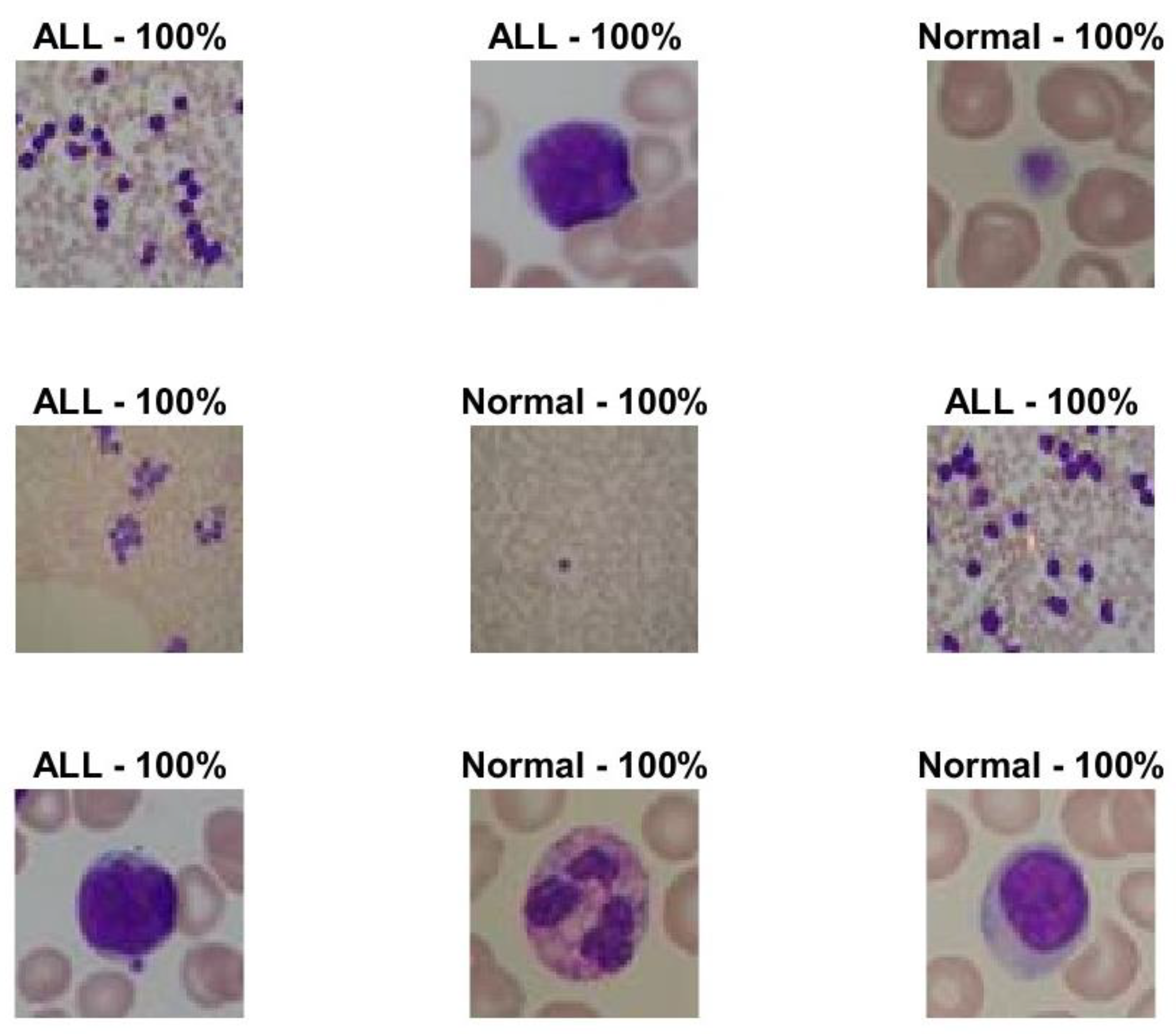
| Optimized Model | 0 | 100% | 100% | 198.33 |
| Methodology | Classifier | Optimization | Dataset | AC | Paper |
|---|---|---|---|---|---|
| Features extraction by AlexNet, CaffeNet, and VGG-f then feature fusion and selection by Gain Ratio algorithm. | SVM | - | ALL-IDB | 99.2 | [8] |
| Features extraction by AlexNet, GoogleNet, and SqueezeNet followed by feature fusion. | SVM | - | ALL-IDB 2 | 98.2 | [22] |
| Features extraction by DarkNet and ShuffleNet followed by feature fusion and selection by Principal Component Analysis | Decision Tree | - | ALL-IDB | 100 | [44] |
| Naïve Bayes | - | 96 | |||
| Feature extraction by VGGNet. Optimal features are selected by a bio-inspired optimizer. | KNN, SVM, Decision Tree, Naive Bayes | Salp Swarm Optimization | ALL-IDB 2 | 96.1 | [53] |
| Hand crafted features from input images and optimal feature selection by an optimizer. | Ensemble of classical ML classifiers | Social Spider Optimization | ALL-IDB 2 | 95.2 | [54] |
| Image segmentation using Sparse Fuzzy C-Means clustering and optimized CNN for classification. | Customized CNN | Grey wolf-based Jaya Optimization | ALL-IDB 2 | 93.5 | [55] |
| Attention-based Long-Short Term Memory for classification after feature selection. | ABiLSTM | Competitive Swarm Optimization | ALL-IDB 1 | 96 | [56] |
| Bayesian-optimized CNN for classification | Customized CNN (BO-ALLCNN) | Bayesian Optimization | ALL-IDB | 100 | Proposed study |
Publisher’s Note: MDPI stays neutral with regard to jurisdictional claims in published maps and institutional affiliations. |
© 2022 by the authors. Licensee MDPI, Basel, Switzerland. This article is an open access article distributed under the terms and conditions of the Creative Commons Attribution (CC BY) license (https://creativecommons.org/licenses/by/4.0/).
Share and Cite
Atteia, G.; Alhussan, A.A.; Samee, N.A. BO-ALLCNN: Bayesian-Based Optimized CNN for Acute Lymphoblastic Leukemia Detection in Microscopic Blood Smear Images. Sensors 2022, 22, 5520. https://doi.org/10.3390/s22155520
Atteia G, Alhussan AA, Samee NA. BO-ALLCNN: Bayesian-Based Optimized CNN for Acute Lymphoblastic Leukemia Detection in Microscopic Blood Smear Images. Sensors. 2022; 22(15):5520. https://doi.org/10.3390/s22155520
Chicago/Turabian StyleAtteia, Ghada, Amel A. Alhussan, and Nagwan Abdel Samee. 2022. "BO-ALLCNN: Bayesian-Based Optimized CNN for Acute Lymphoblastic Leukemia Detection in Microscopic Blood Smear Images" Sensors 22, no. 15: 5520. https://doi.org/10.3390/s22155520
APA StyleAtteia, G., Alhussan, A. A., & Samee, N. A. (2022). BO-ALLCNN: Bayesian-Based Optimized CNN for Acute Lymphoblastic Leukemia Detection in Microscopic Blood Smear Images. Sensors, 22(15), 5520. https://doi.org/10.3390/s22155520