
Smart Strawberry Farming Using Edge Computing and IoT


Abstract
:1. Introduction
2. Background
2.1. Wireless Sensor Network
2.2. Computer Vision
2.3. Machine Learning
3. Literature Review
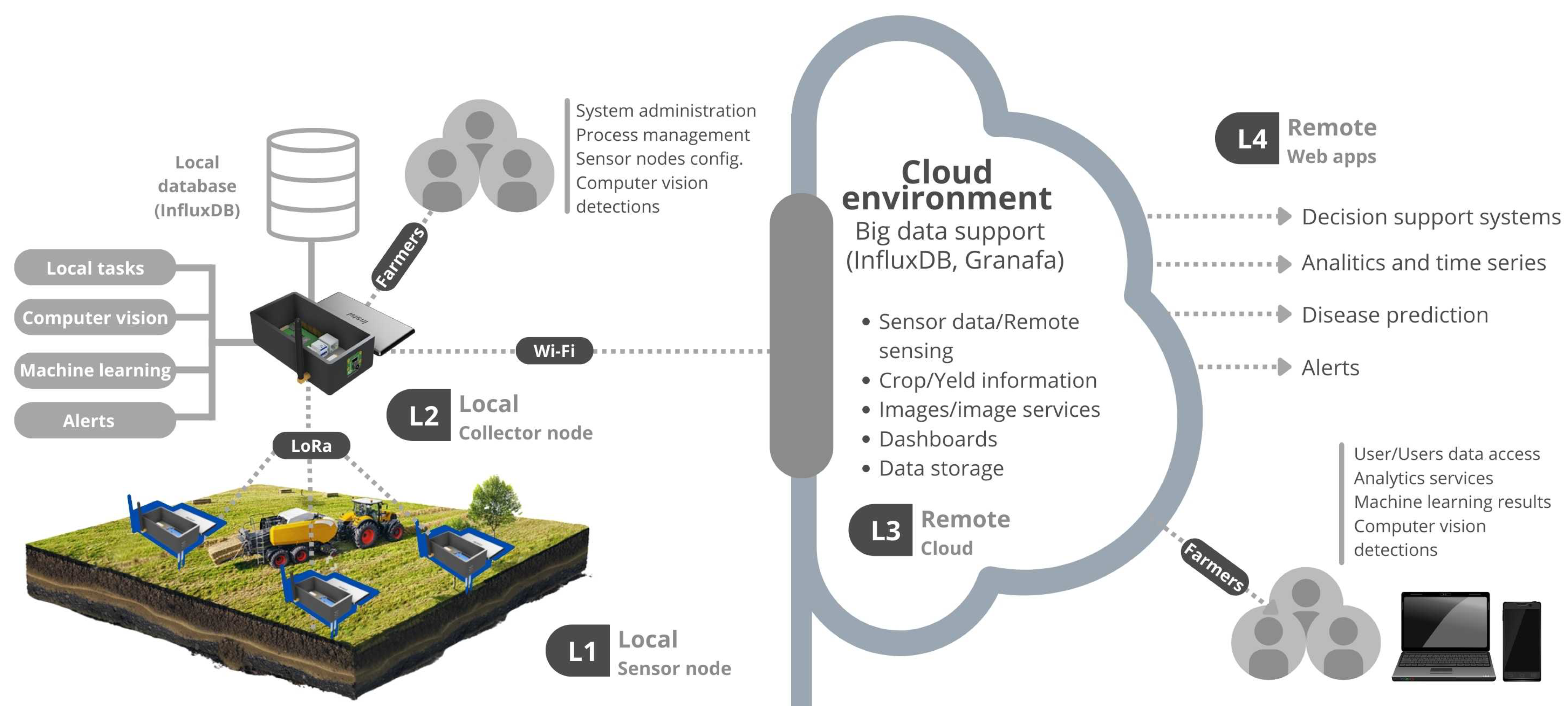
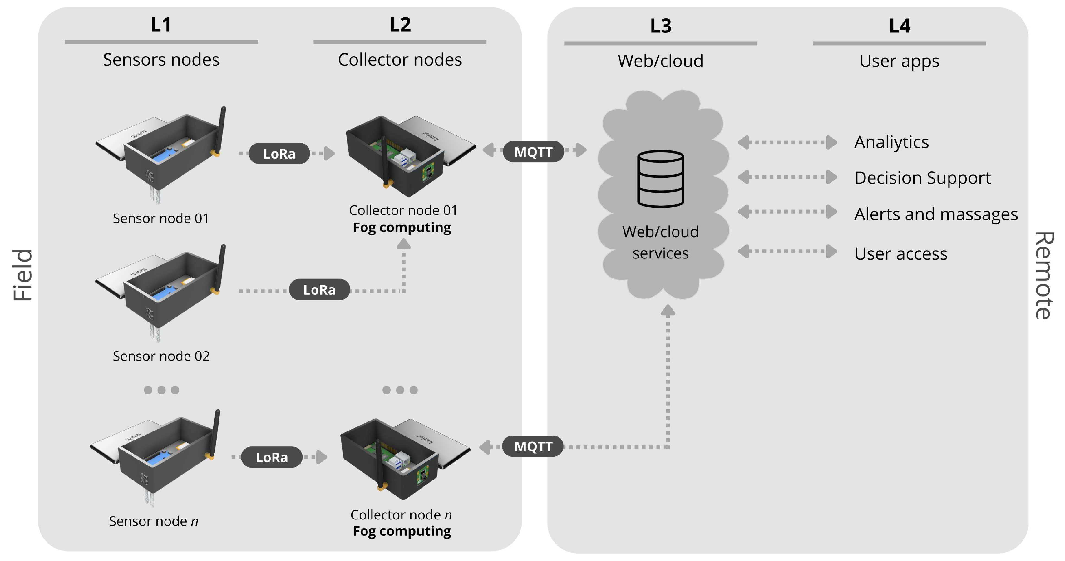
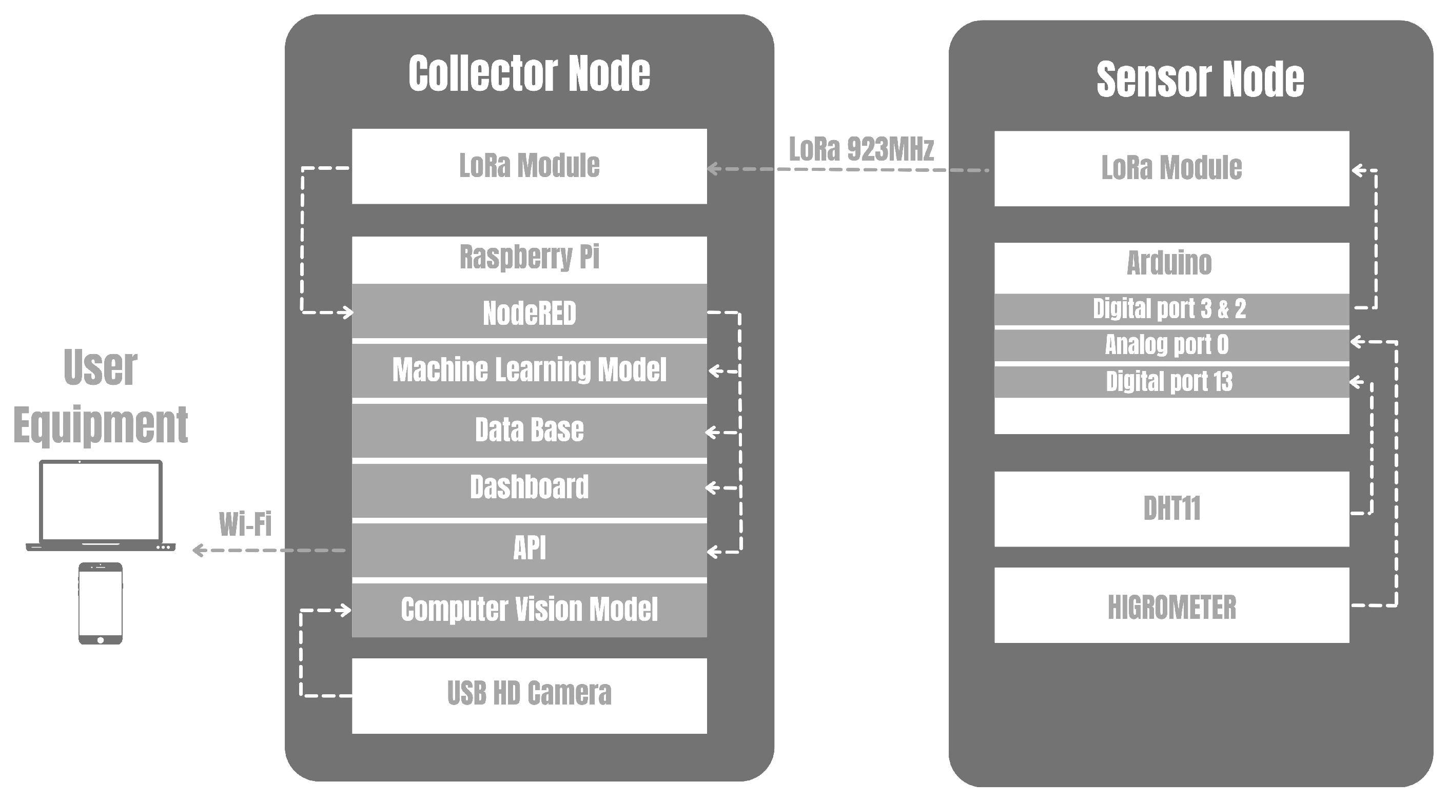
4. Proposed IoT Plataform
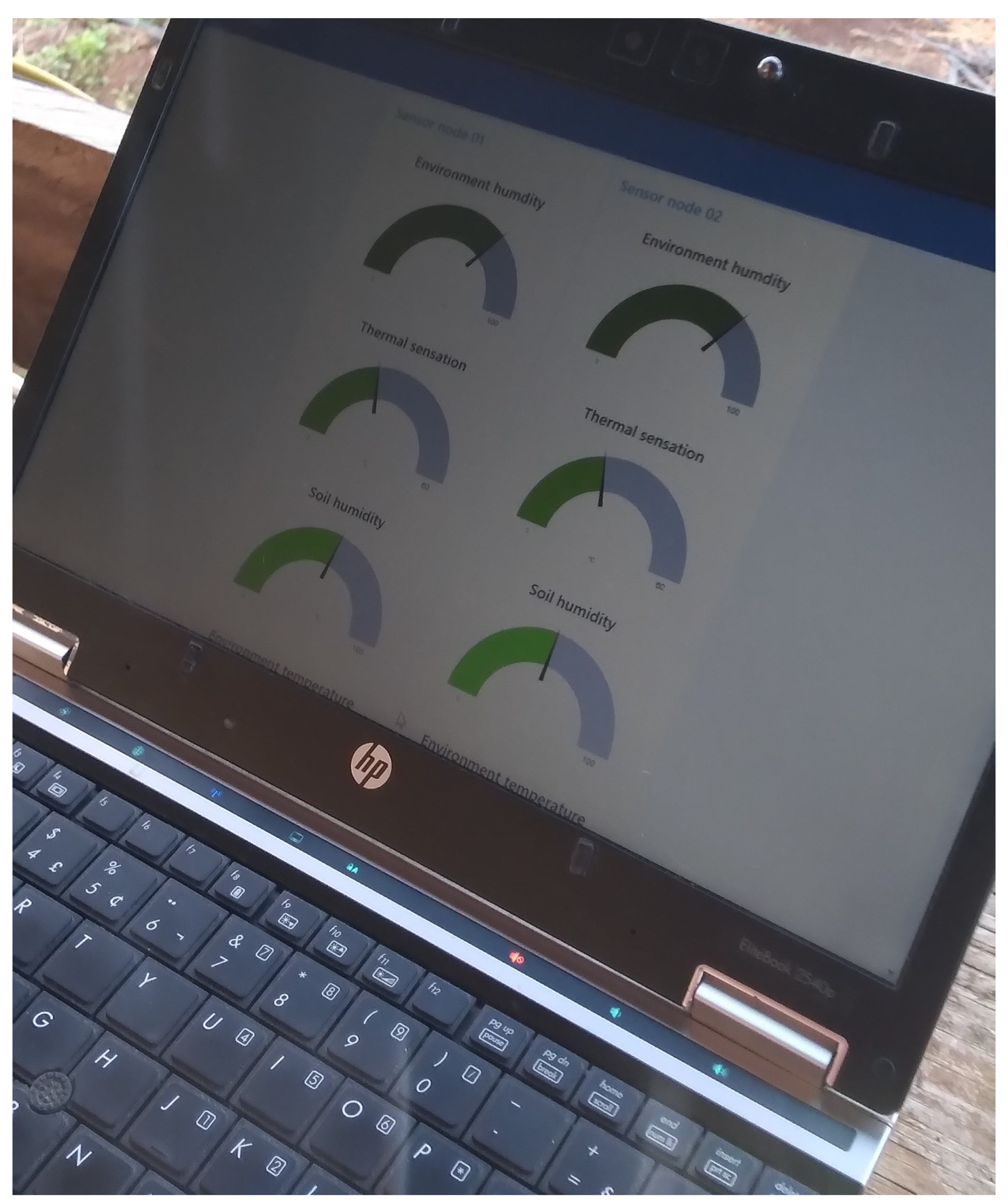
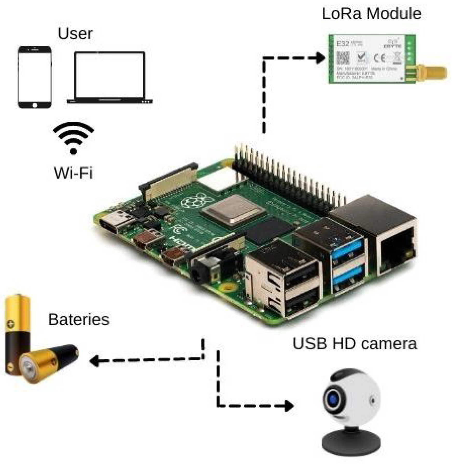
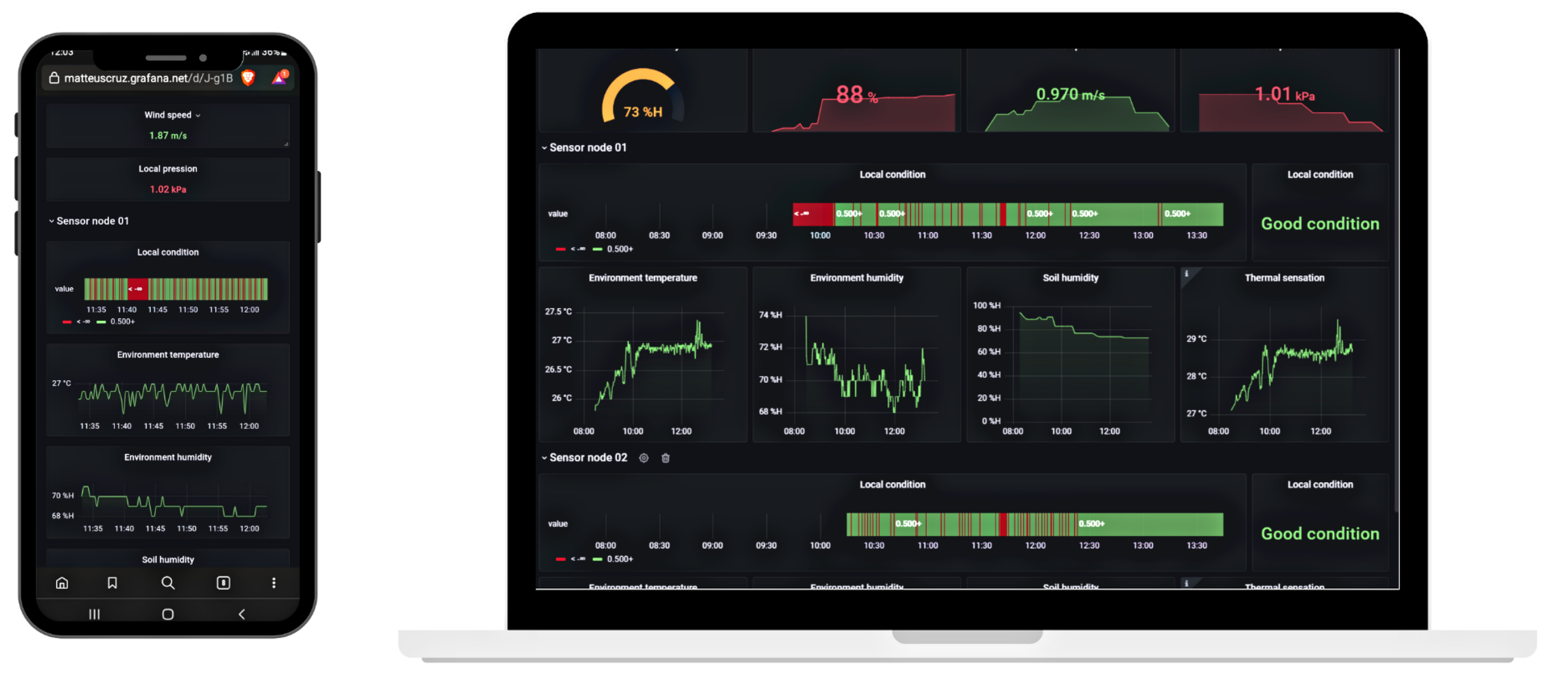
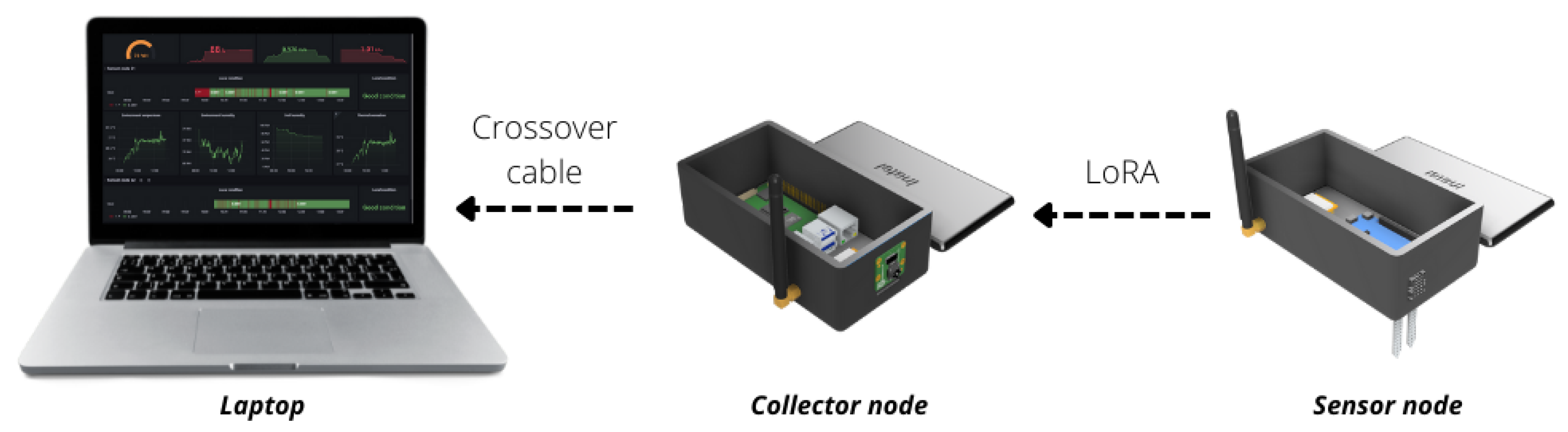
4.1. The IoT Platform
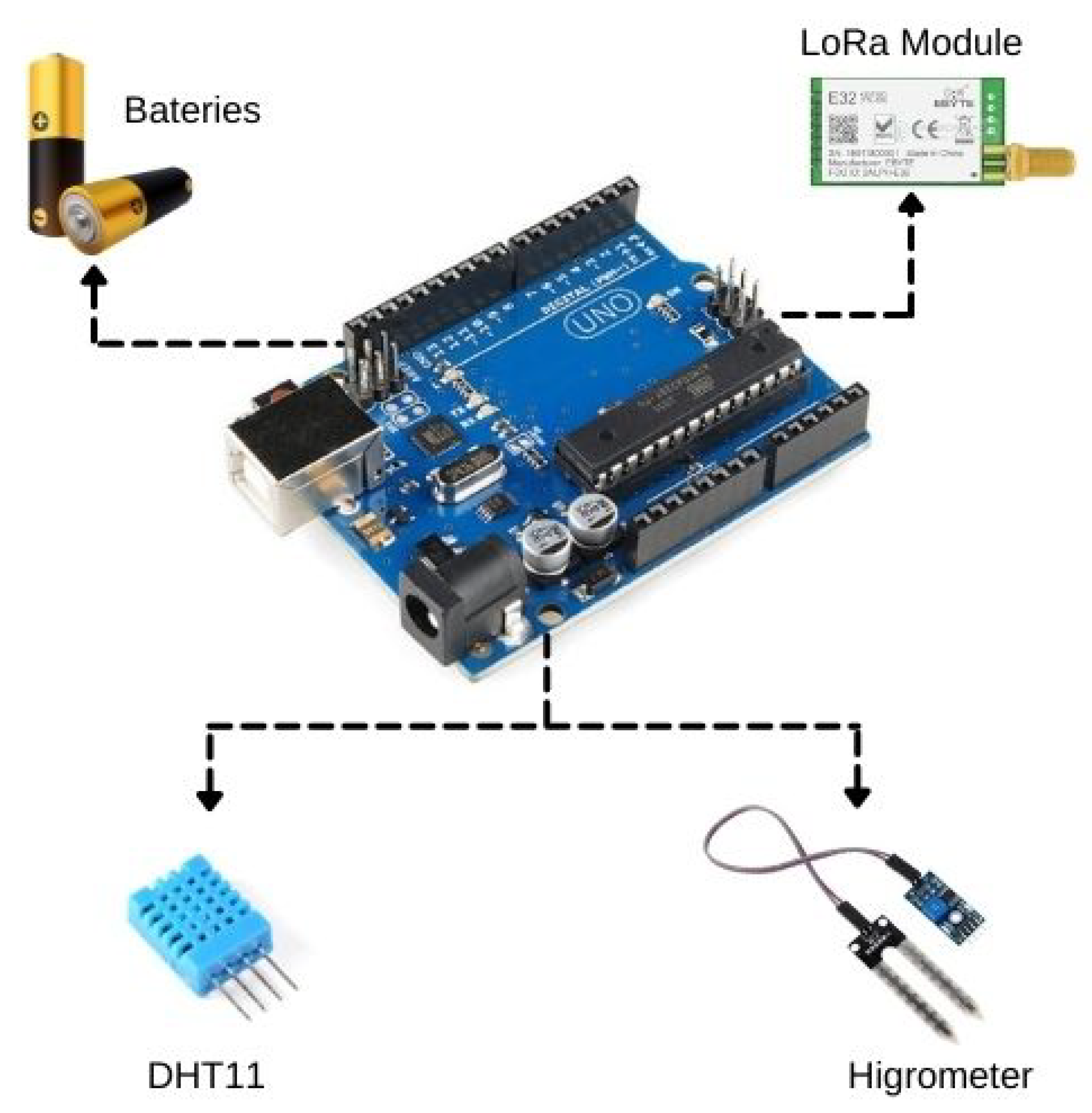
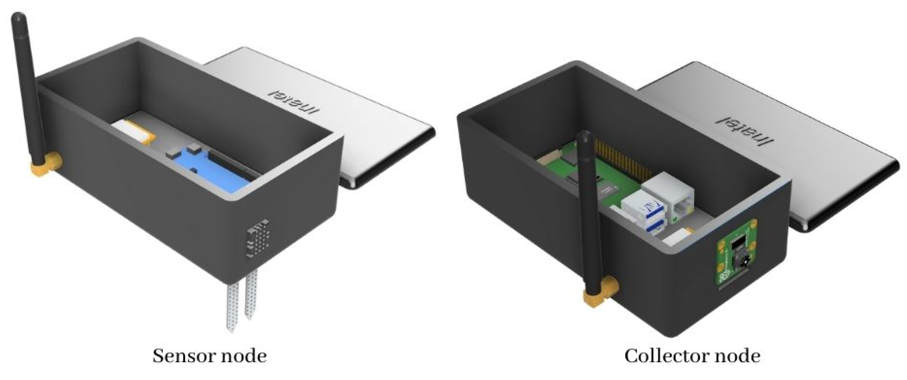
4.1.1. Detailed Overview of the Hardware
- Raspberry Pi 4B: A only computer board with 4 GB of RAM, Broadcom BCM2711, Quad-core Cortex-A72 (ARM v8) 64-bit SoC @ 1.5 GHz. The board presents a native Wi-Fi connection.
- Radio Frequency Wireless module LoRa 915 MHz [flip-flop]. A Lord module that operates in the 850.125–930.125 MHz range, with reception sensibility of −147 dBm and transfer range of 2.4–62.5 Kbps.
- HD USB Camera: An 1080p camera compatible with Windows and Linux systems, USB 2.0.
- Humidity and temperature sensor DHT11: It is a sensor of relative humidity and environment temperature. The sensor can capture relative humidity in a range of 20 to 90%. DHT11 also captures temperature on 0 to 50 °C with a precision of ±5.0% UR and ± 2.0 ºC with a time to respond equal to 2 s;
- Soil humidity sensor hygrometer: Soil humidity sensor is based on LM393 comparator with easy installation, low price, and large availability;
4.1.2. Detailed Overview of Software
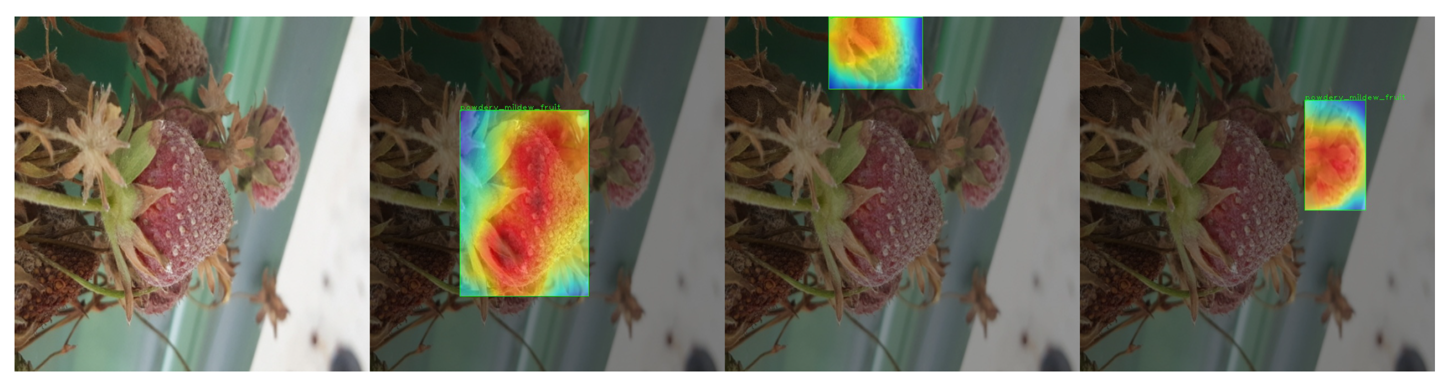
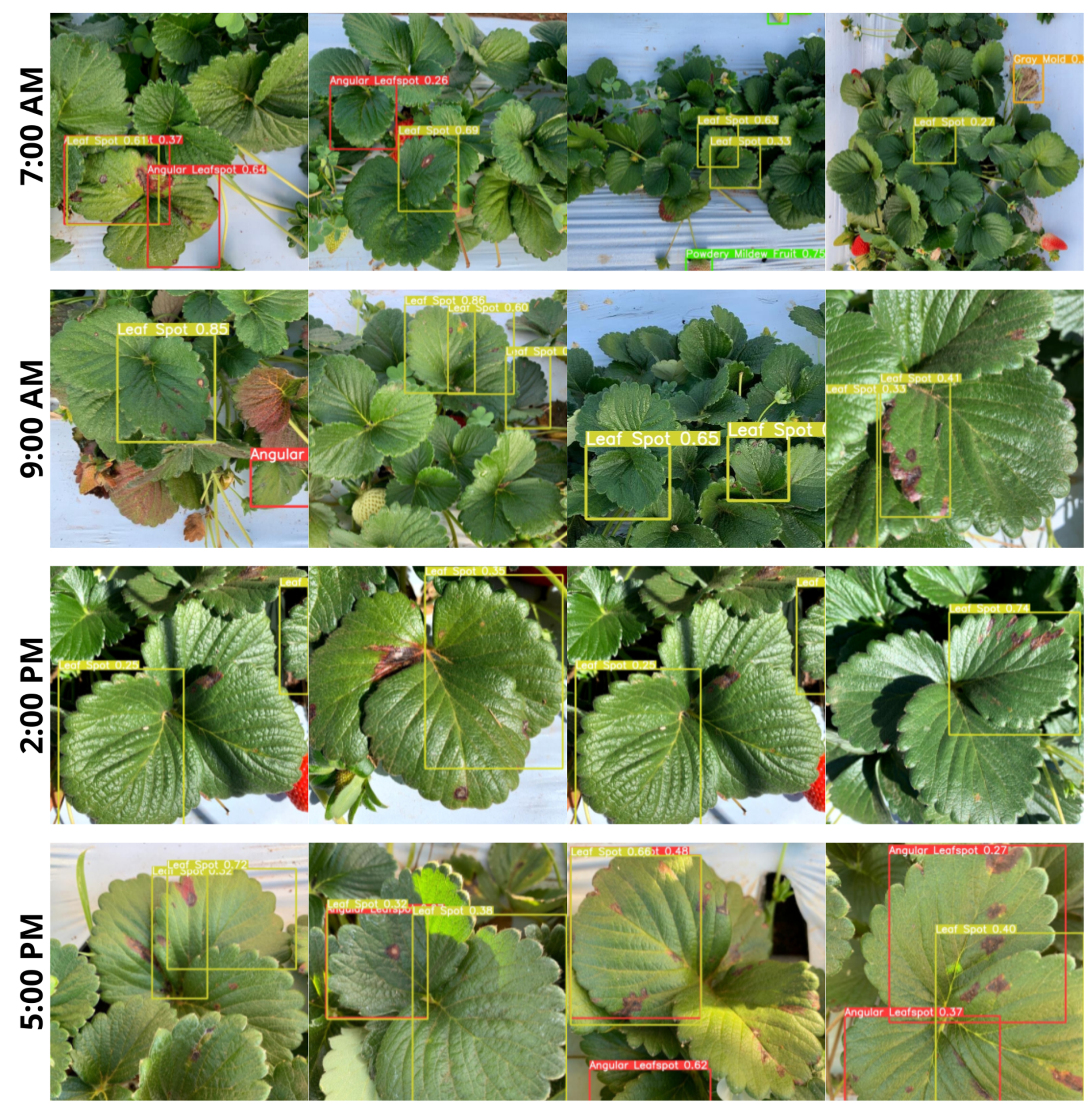
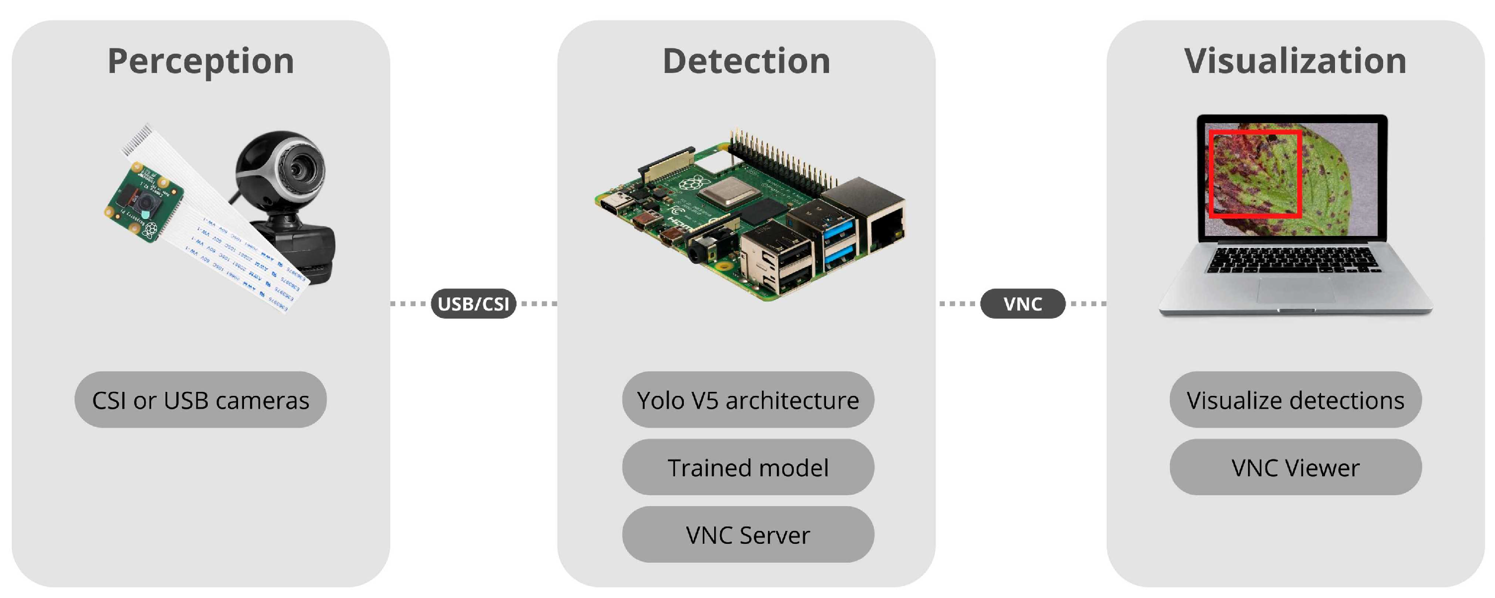
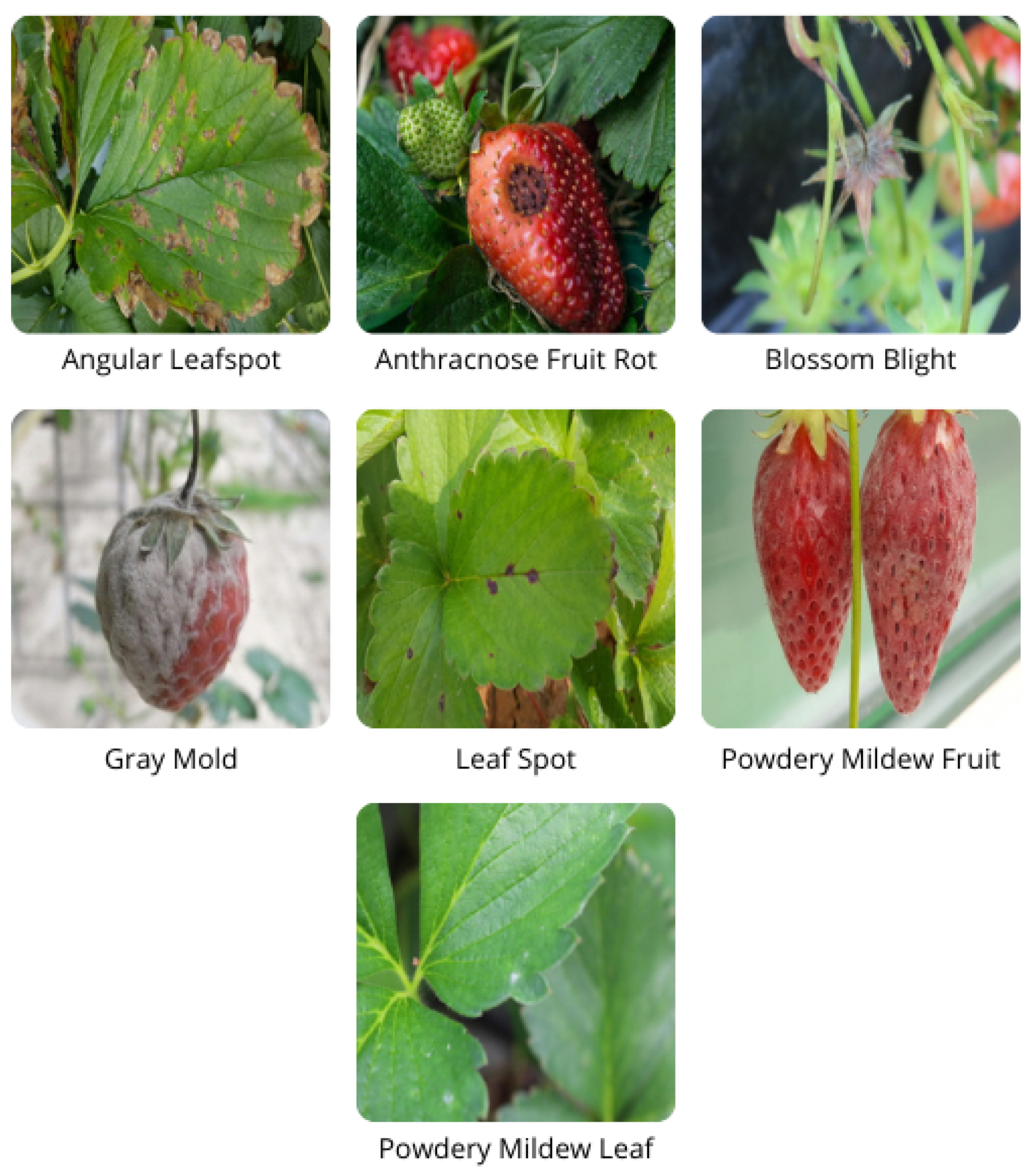
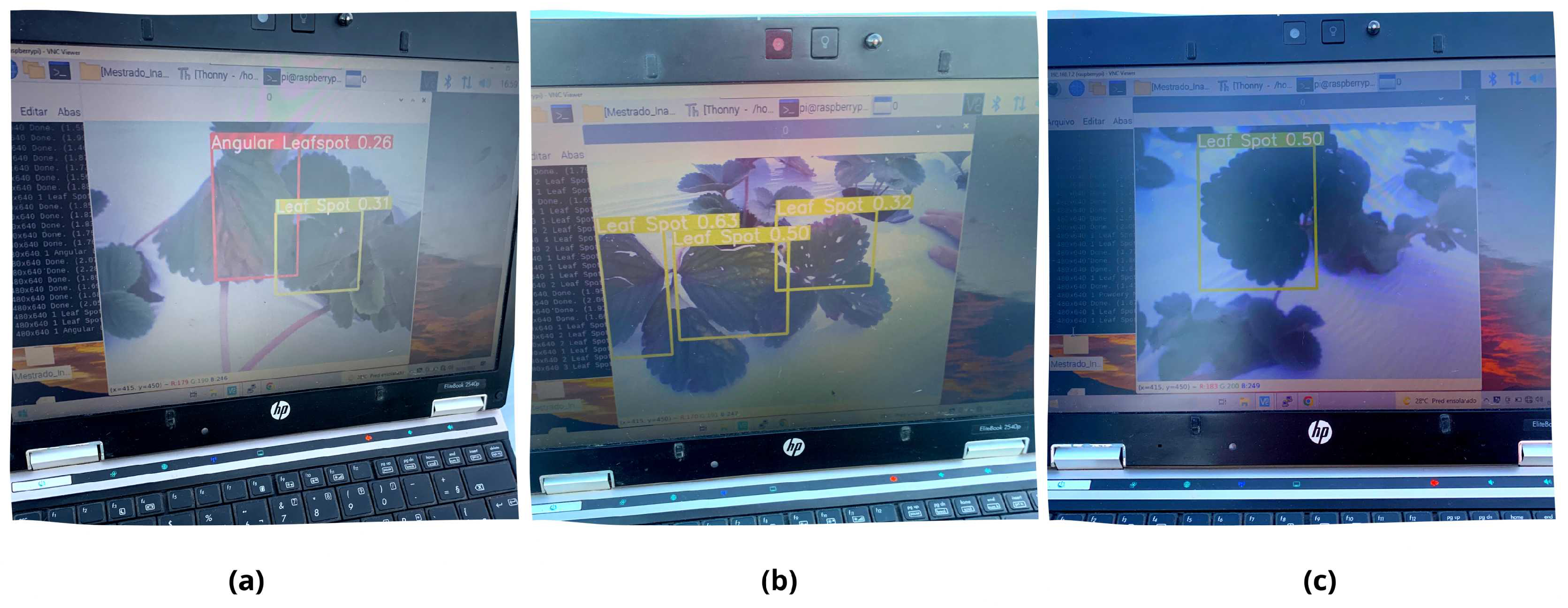
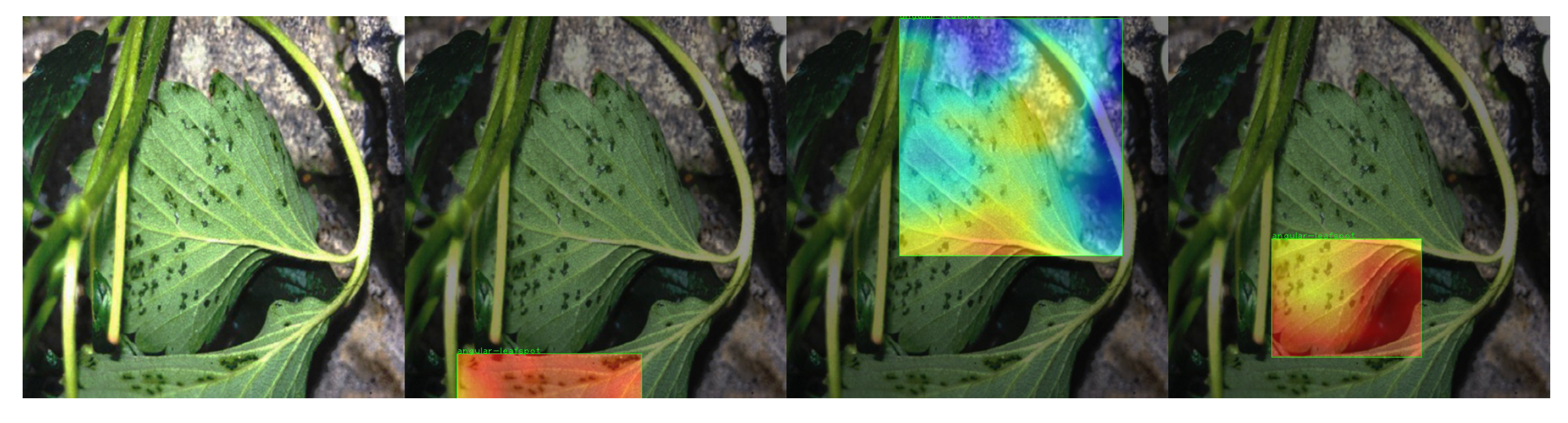
4.2. Computer Vision System for Disease Detection
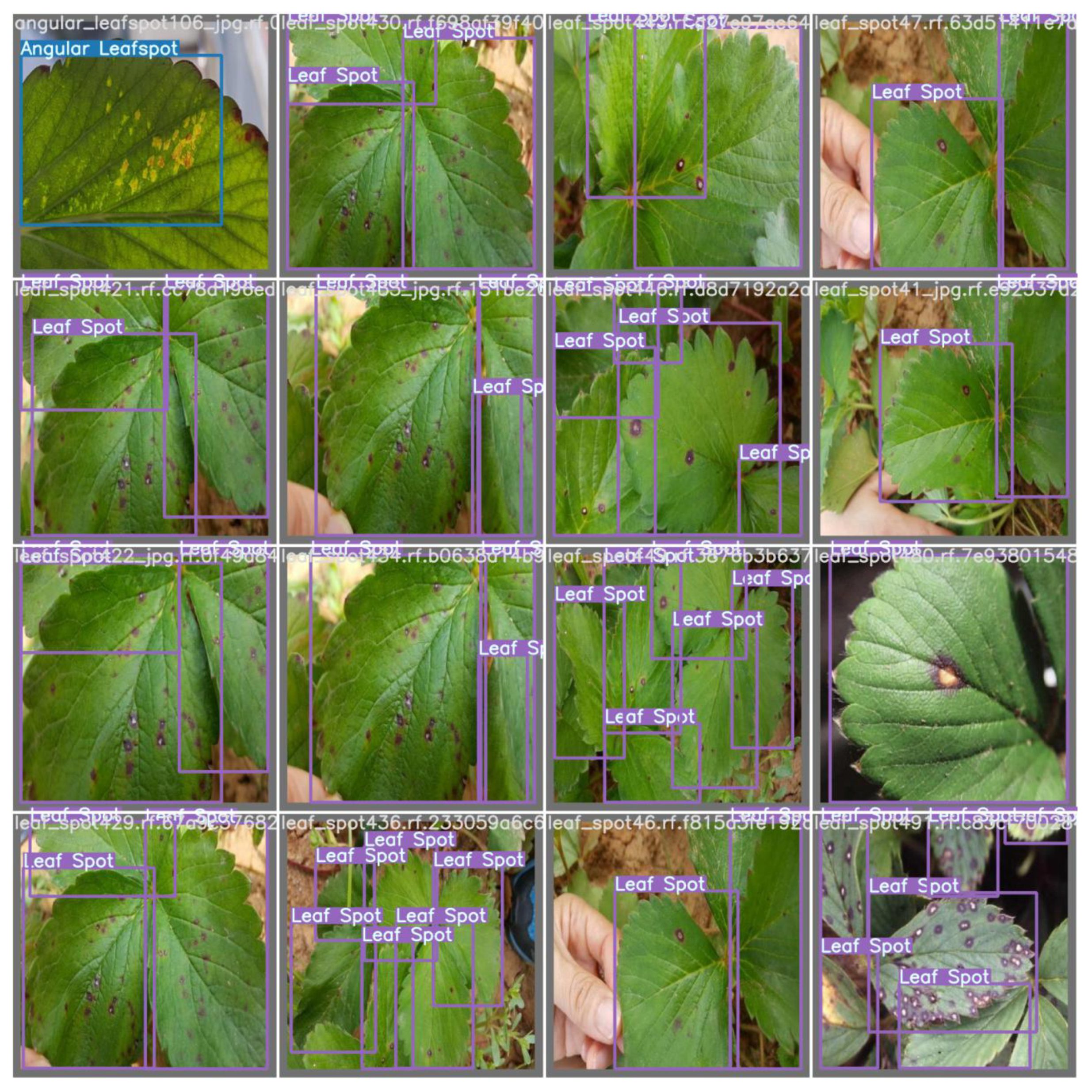
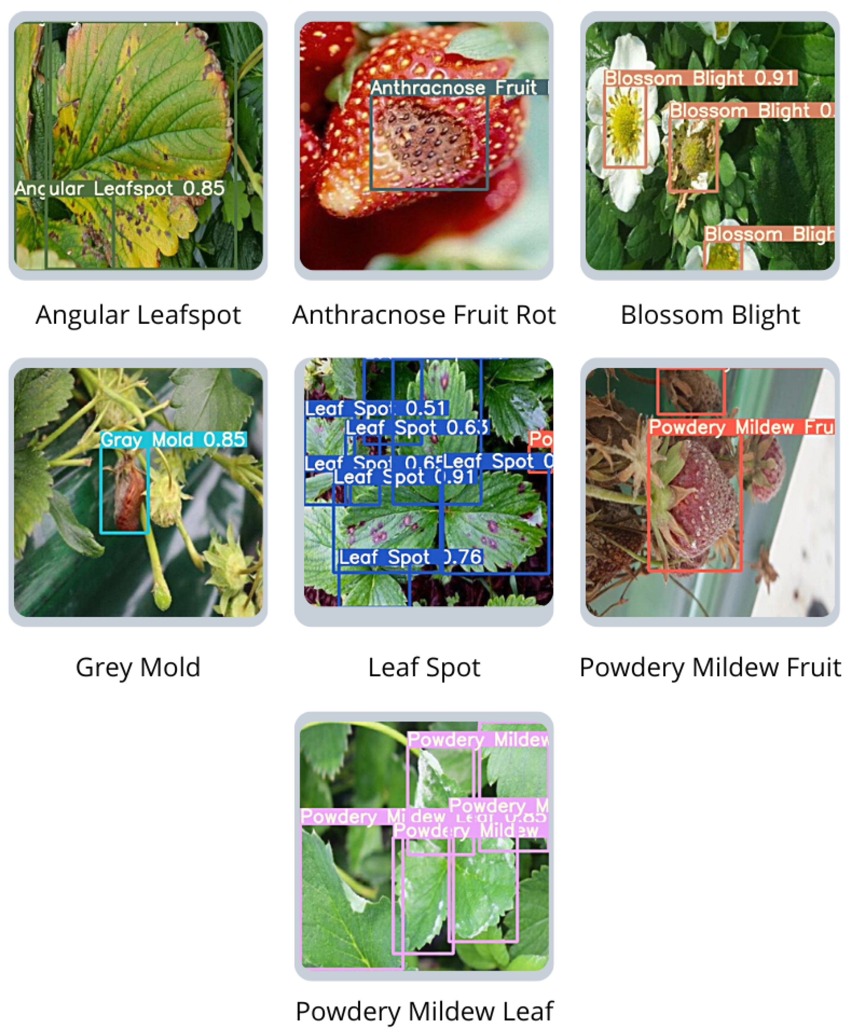
- Angular Leaf Spot: Known as “bacterial stain”, the disease is caused by Xanthomonas fragariae bacteria. The name is given by the appearance of light green, increasing their size later until they become visible on the sheet.
- Anthracnose Fruit Rot: It is a rot caused by agents such as Colletotrichum fragariae, C. acutatum, and C. gloeoporioides. The rot is generated when the plant is submitted to high temperature and humidity conditions.
- Blossom Blight: Disease symptoms began with gray sporulation of the fungus on the stigmas and anthers of strawberry flowers, followed by necrosis and complete flower abortion.
- Grey Mold: Caused by the Botrytis cinerea Pers. F. fungi or simply Botrytis. The name Gray Mold is given to the appearance of gray color mold formed in the leaf and calyx, which may affect the fruit.
- Leaf Spot: Known as “Mycospherella spot”, the disease is caused by Mycosphaerella fragariae fungi, and it is one of the most common diseases on the strawberry. The fungi attack mainly the leaflets, presenting a purple color that posterior develops into a brown color.
- Powdery Mildew Leaf: Caused by the Sphaerotheca macularis fungi. The powdery mildew is caused when the plantation is submitted to a dry and hot climate. Manifestation is given by the apparition of whitish spots on the inferior face of the leaf. It also affects the fruits and can be observed by the fruit’s discoloration and spots.
- Powdery Mildew Fruit: It is caused by Sphaerotheca macularis fungi, affects the fruits, and can be observed by the fruit’s discoloration and spots.
4.2.1. Yolo v5 Architecture
4.2.2. Dataset and Training Phases
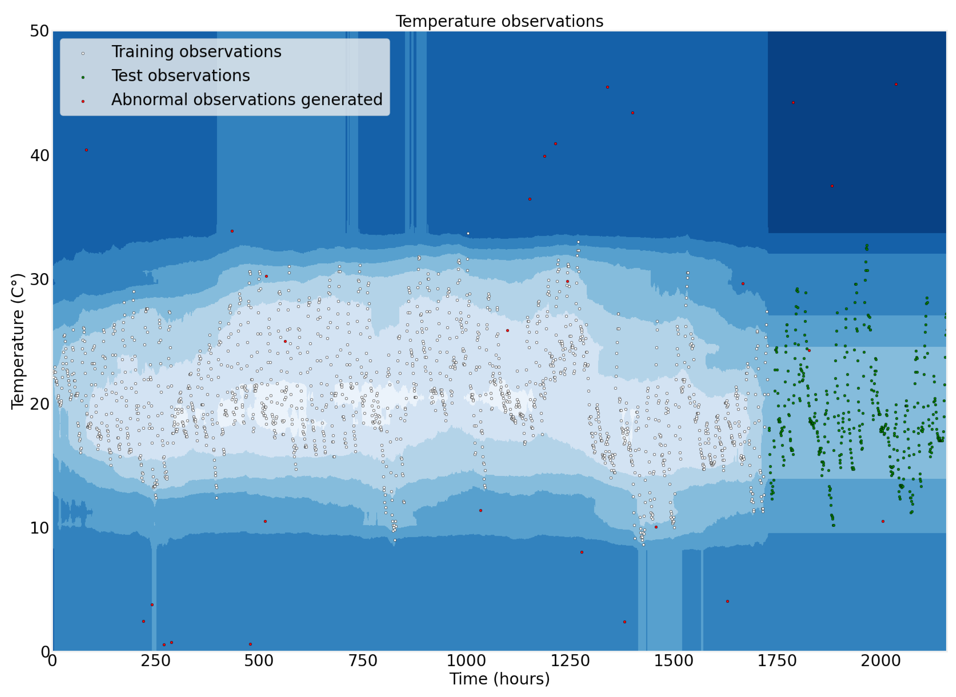
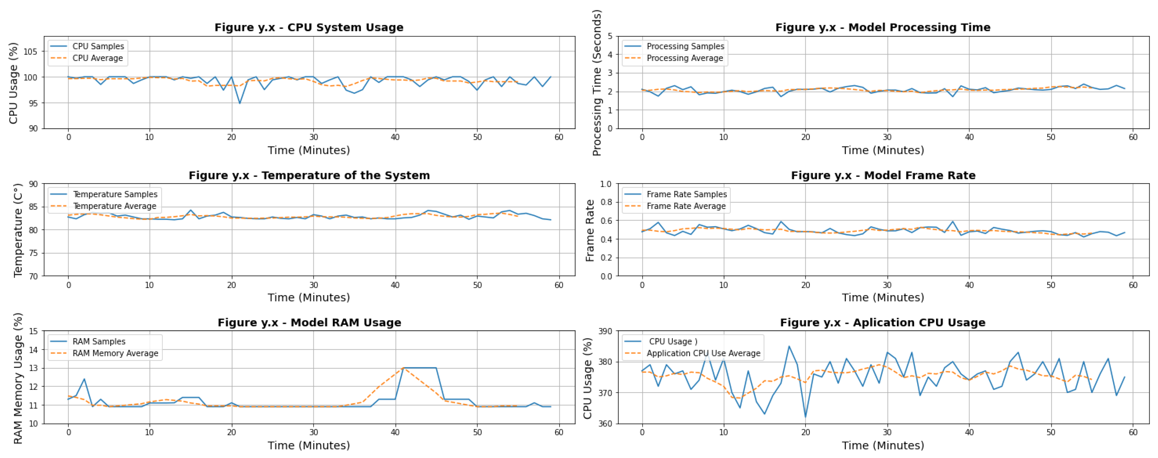
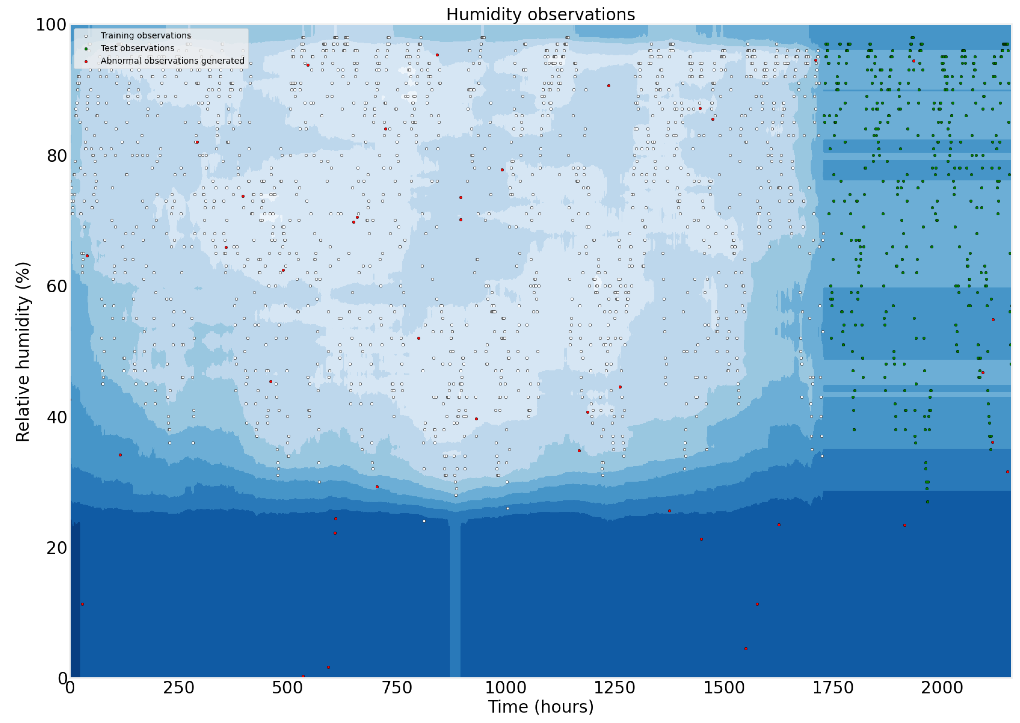
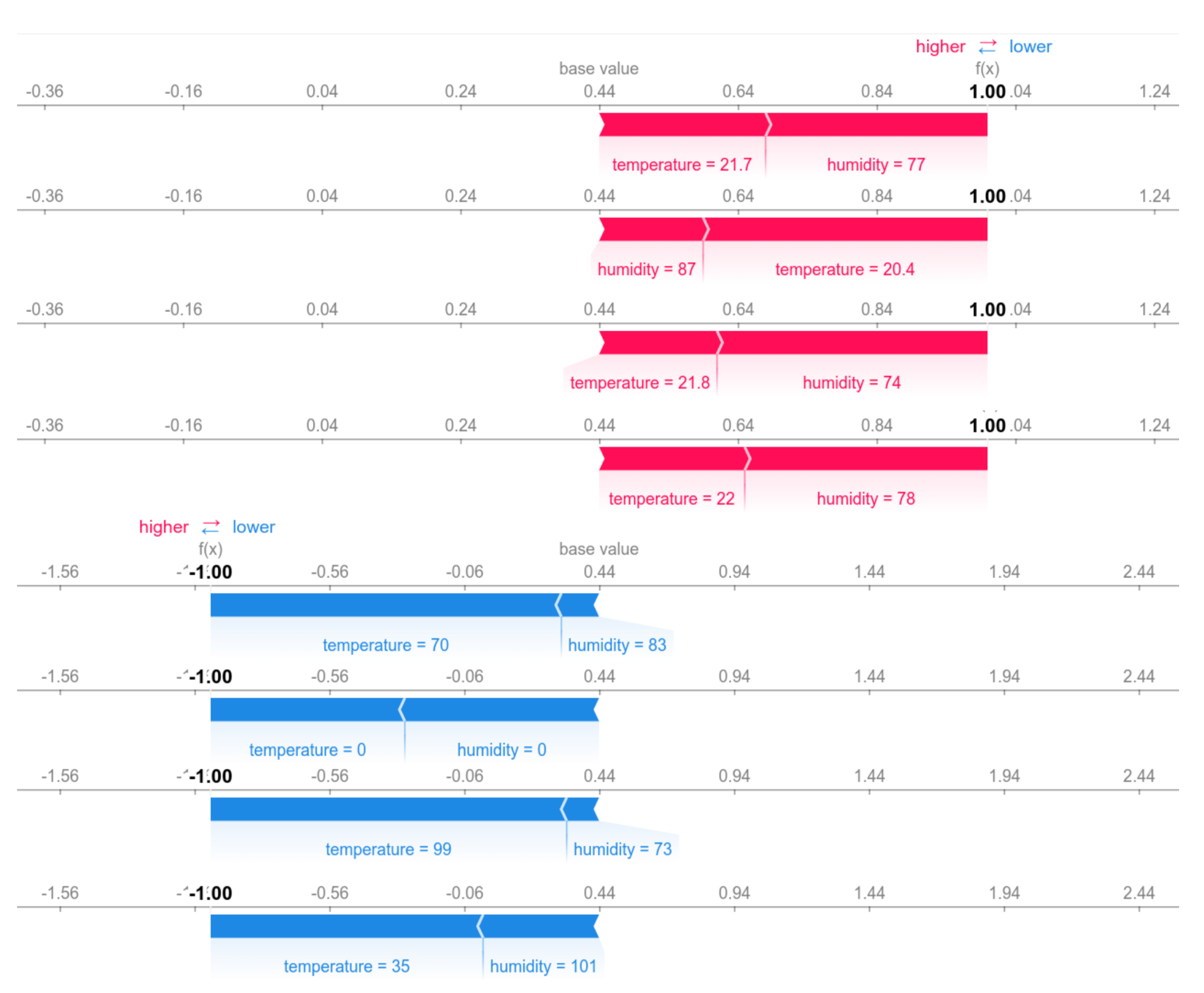
4.3. Machine Learning
Implementation and Working Pipeline
- Bootstrap: False;
- Contamination: Auto;
- Maximum Features: 1.0;
- Maximum Samples: 100;
- Number of Estimators: 100;
- Number of Jobs: None;
- Verbose: 0.
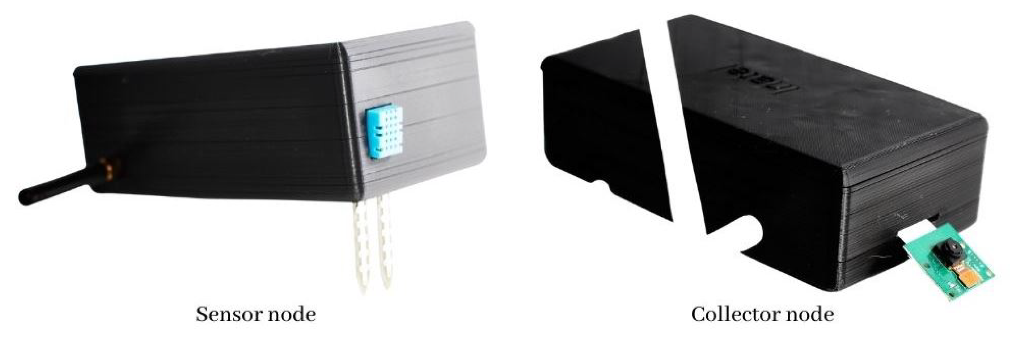
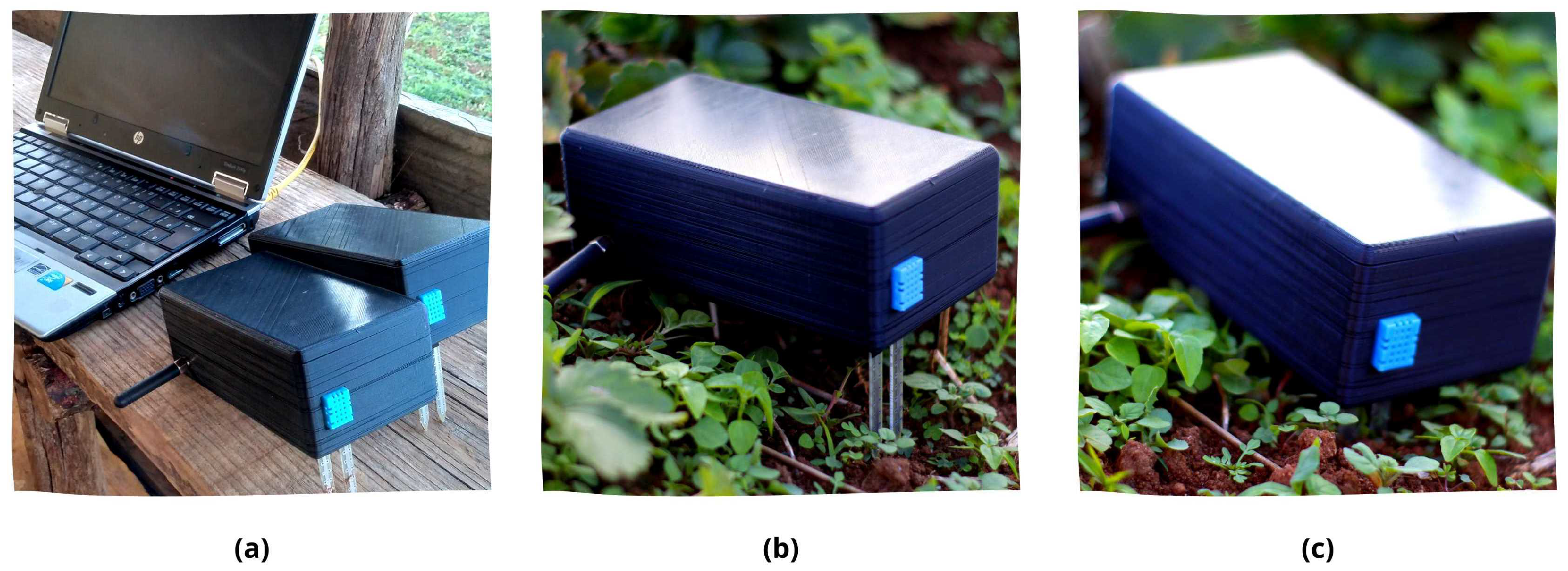
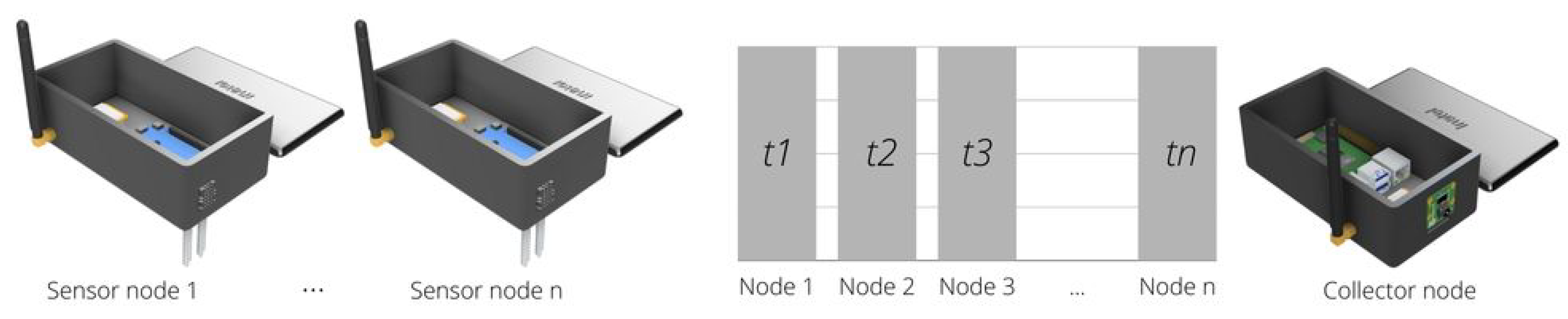
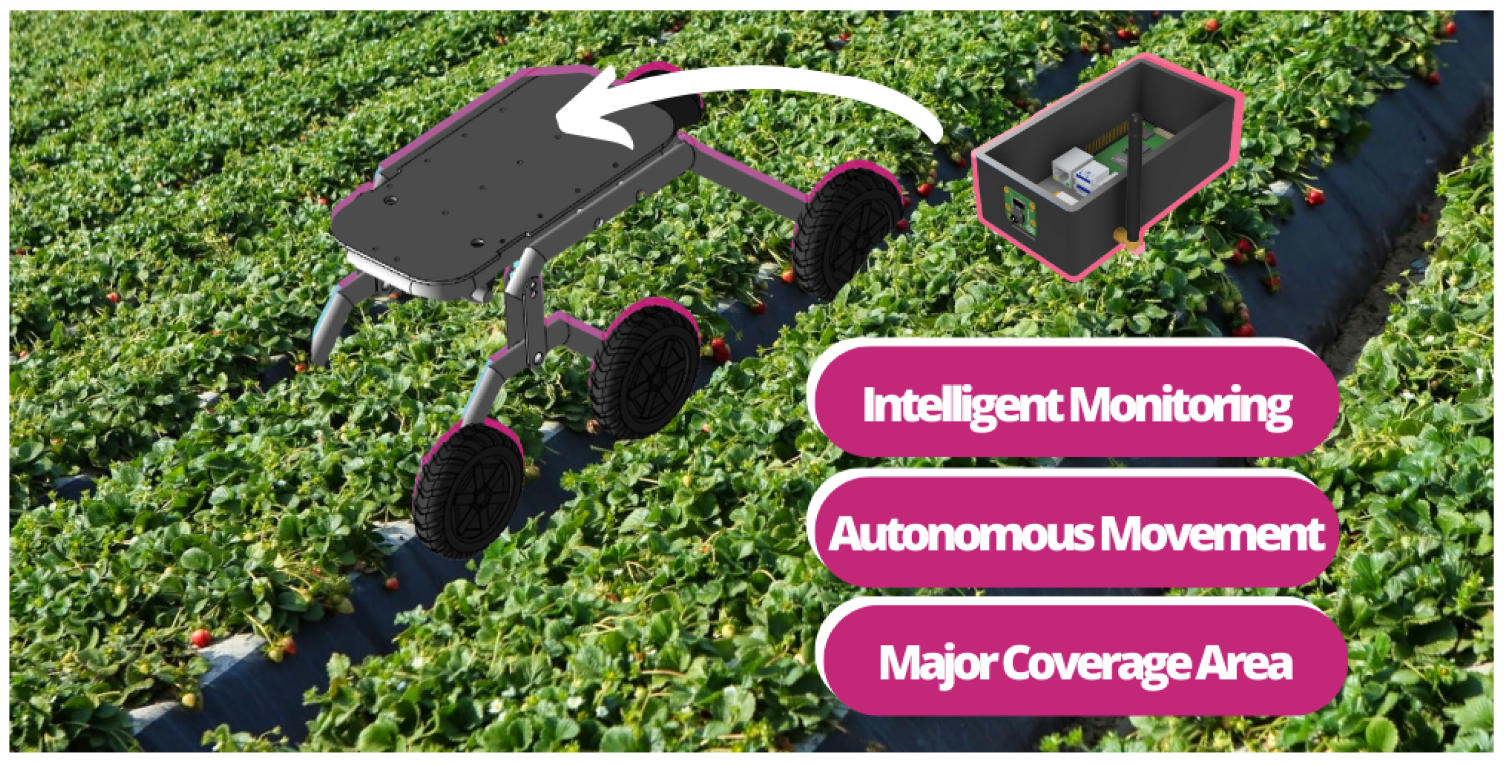
4.4. Encapsulation
4.5. Cost Analysis
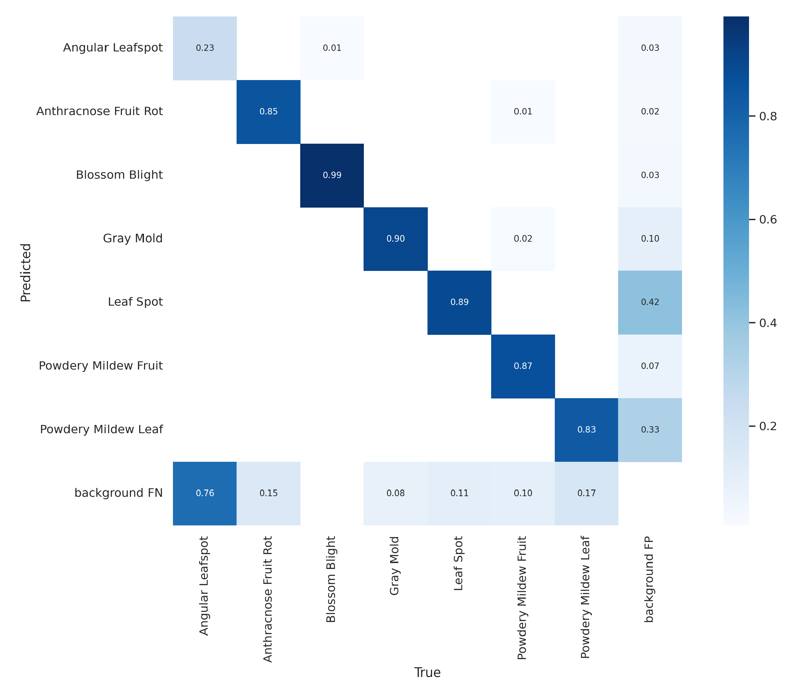
5. Results
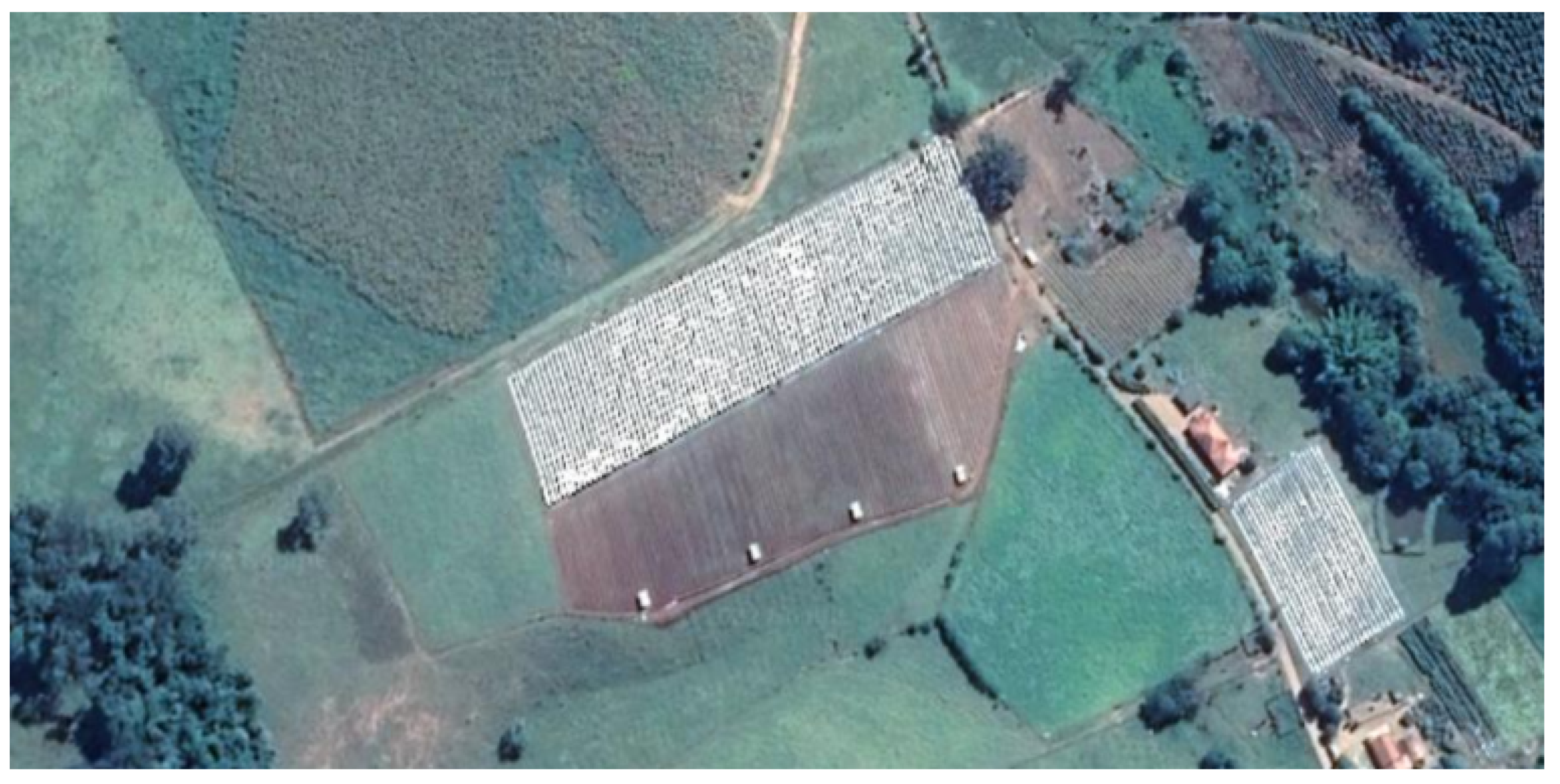
5.1. Case of Study
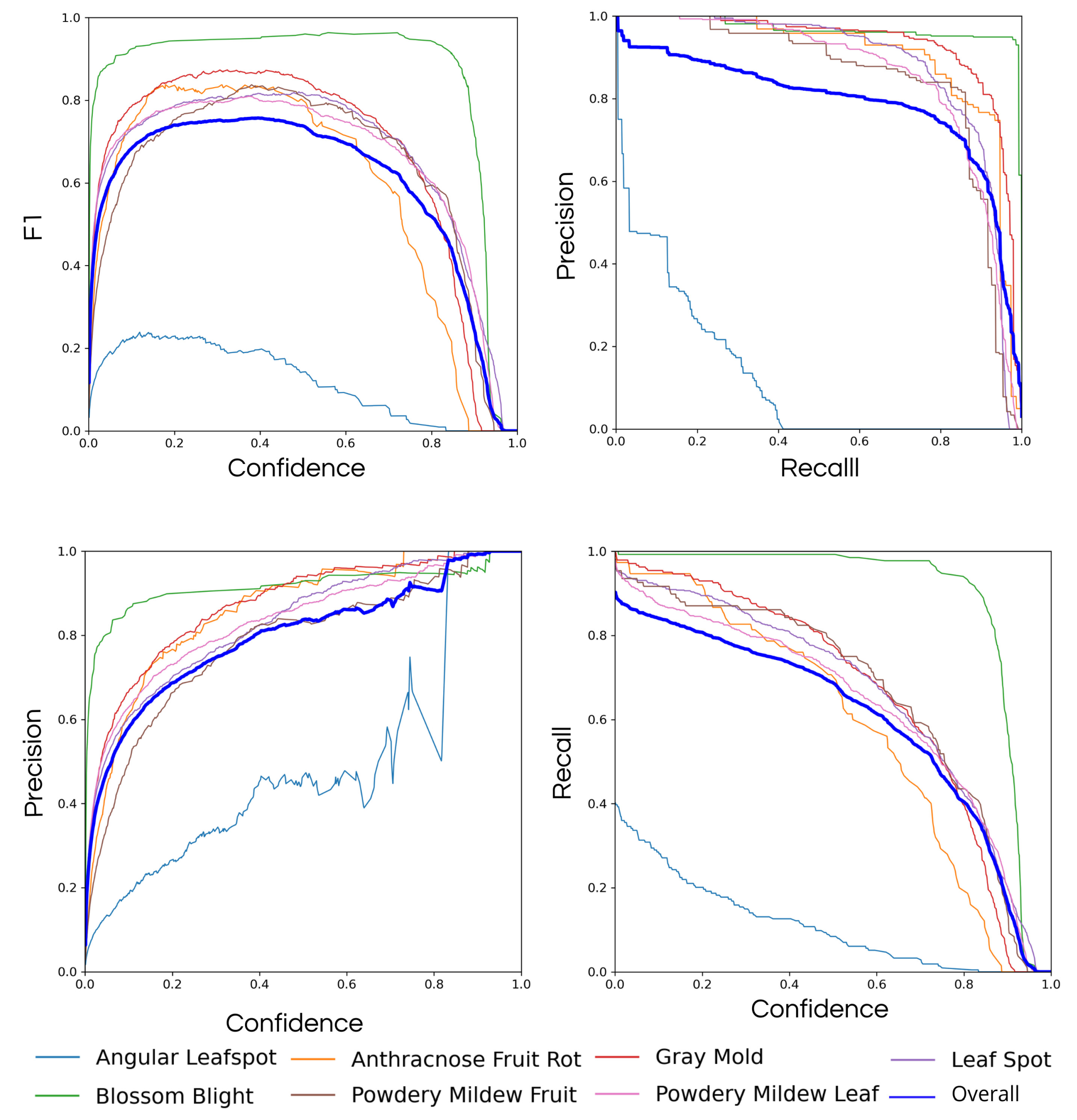
Computer Vision
- Mean average precision (mAP): The metric presents the mean of the average precision (AP), in which AP is represented by the area below the curve.
- Precision: Relation of all the classifications by the model to the correct ones. In general, it is used in situations where false positives have more weight than false negatives;
- Recall: Relation between all the true positives by the sum of true positive and false negative. It is like precision but used in situations where the false negatives are considered more harmful than the false positives.
- Accuracy: Tells about the general performance of the model, being the relation of the correct by all the classifications performed by the model. Accuracy is a good general sign of the performance of the model.
- Box loss: Measures how close the bounding box is from the true box.
5.2. Machine Learning
6. Conclusions
Author Contributions
Funding
Data Availability Statement
Conflicts of Interest
References
- Hytönen, T.; Graham, J.; Harrison, R. (Eds.) The Genomes of Rosaceous Berries and Their Wild Relatives; Springer International Publishing: Cham, Switzerland, 2018. [Google Scholar] [CrossRef] [Green Version]
- Soares, V.F.; Velho, A.C.; Carachenski, A.; Astolfi, P.; Stadnik, M.J. First Report of Colletotrichum karstii Causing Anthracnose on Strawberry in Brazil. Plant Dis. 2021, 105, 3295. [Google Scholar] [CrossRef] [PubMed]
- Li, Y.; Wang, H.; Dang, L.M.; Sadeghi-Niaraki, A.; Moon, H. Crop pest recognition in natural scenes using convolutional neural networks. Comput. Electron. Agric. 2020, 169, 105174. [Google Scholar] [CrossRef]
- Hancock, J.F. Disease and pest management. In Strawberries; CABI: Wallingford, UK, 2020; pp. 171–209. [Google Scholar] [CrossRef]
- Kim, K.H.; Kabir, E.; Jahan, S.A. Exposure to pesticides and the associated human health effects. Sci. Total Environ. 2017, 575, 525–535. [Google Scholar] [CrossRef] [PubMed]
- Patel, A.; Lee, W.S.; Peres, N.A.; Fraisse, C.W. Strawberry plant wetness detection using computer vision and deep learning. Smart Agric. Technol. 2021, 1, 100013. [Google Scholar] [CrossRef]
- Feng, Q.; Zheng, W.; Qiu, Q.; Kai, J.; Rui, G. Study on strawberry robotic harvesting system. In Proceedings of the 2012 IEEE International Conference on Computer Science and Automation Engineering (CSAE), Zhangjiajie, China, 25–27 May 2012; Volume 1, pp. 320–324. [Google Scholar] [CrossRef]
- Habib, M.T.; Raza, D.M.; Islam, M.M.; Victor, D.B.; Arif, M.A.I. Applications of Computer Vision and Machine Learning in Agriculture: A State-of-the-Art Glimpse. In Proceedings of the 2022 International Conference on Innovative Trends in Information Technology (ICITIIT), Kerala, India, 12–13 February 2022; pp. 1–5. [Google Scholar] [CrossRef]
- Kumar, A.; Joshi, R.C.; Dutta, M.K.; Jonak, M.; Burget, R. Fruit-CNN: An Efficient Deep learning-based Fruit Classification and Quality Assessment for Precision Agriculture. In Proceedings of the 2021 13th International Congress on Ultra Modern Telecommunications and Control Systems and Workshops (ICUMT), Brno, Czech Republic, 25–27 October 2021; pp. 60–65. [Google Scholar] [CrossRef]
- Richey, B.; Shirvaikar, M.V. Deep learning based real-time detection of Northern Corn Leaf Blight crop disease using YoloV4. Real-Time Image Process. Deep. Learn. 2021, 11736, 39–45. [Google Scholar] [CrossRef]
- Elhassouny, A.; Smarandache, F. Smart mobile application to recognize tomato leaf diseases using Convolutional Neural Networks. In Proceedings of the 2019 International Conference of Computer Science and Renewable Energies (ICCSRE), Agadir, Morocco, 22–24 July 2019. [Google Scholar] [CrossRef]
- Picon, A.; Seitz, M.; Alvarez-Gila, A.; Mohnke, P.; Ortiz-Barredo, A.; Echazarra, J. Crop conditional Convolutional Neural Networks for massive multi-crop plant disease classification over cell phone acquired images taken on real field conditions. Comput. Electron. Agric. 2019, 167, 105093. [Google Scholar] [CrossRef]
- García, L.; Parra, L.; Jimenez, J.M.; Lloret, J.; Lorenz, P. IoT-Based Smart Irrigation Systems: An Overview on the Recent Trends on Sensors and IoT Systems for Irrigation in Precision Agriculture. Sensors 2020, 20, 1042. [Google Scholar] [CrossRef] [Green Version]
- Dagar, R.; Som, S.; Khatri, S.K. Smart Farming–IoT in Agriculture. In Proceedings of the 2018 International Conference on Inventive Research in Computing Applications (ICIRCA), Coimbatore, India, 11–12 July 2018. [Google Scholar] [CrossRef]
- Jha, R.K.; Kumar, S.; Joshi, K.; Pandey, R. Field monitoring using IoT in agriculture. In Proceedings of the 2017 International Conference on Intelligent Computing, Instrumentation and Control Technologies (ICICICT), Kannur, India, 6–7 July 2017. [Google Scholar] [CrossRef]
- Davcev, D.; Mitreski, K.; Trajkovic, S.; Nikolovski, V.; Koteli, N. IoT agriculture system based on LoRaWAN. In Proceedings of the 2018 14th IEEE International Workshop on Factory Communication Systems (WFCS), Imperia, Italy, 13–15 June 2018. [Google Scholar] [CrossRef]
- Mat, I.; Kassim, M.R.M.; Harun, A.N.; Yusoff, I.M. IoT in Precision Agriculture applications using Wireless Moisture Sensor Network. In Proceedings of the 2016 IEEE Conference on Open Systems (ICOS), Langkawi, Malaysia, 10–12 October 2016. [Google Scholar] [CrossRef]
- Baranwal, T.; Nitika; Pateriya, P.K. Development of IoT based smart security and monitoring devices for agriculture. In Proceedings of the 2016 6th International Conference—Cloud System and Big Data Engineering (Confluence), Noida, India, 14–15 January 2016. [Google Scholar] [CrossRef]
- Mamdouh, M.; Elrukhsi, M.A.I.; Khattab, A. Securing the Internet of Things and Wireless Sensor Networks via Machine Learning: A Survey. In Proceedings of the 2018 International Conference on Computer and Applications (ICCA), Beirut, Lebanon, 25–26 August 2018. [Google Scholar] [CrossRef]
- Voulodimos, A.; Doulamis, N.; Doulamis, A.; Protopapadakis, E. Deep Learning for Computer Vision: A Brief Review. Comput. Intell. Neurosci. 2018, 2018, 7068349. [Google Scholar] [CrossRef]
- Tian, H.; Wang, T.; Liu, Y.; Qiao, X.; Li, Y. Computer vision technology in agricultural automation —A review. Inf. Process. Agric. 2020, 7, 1–19. [Google Scholar] [CrossRef]
- Patrício, D.I.; Rieder, R. Computer vision and artificial intelligence in precision agriculture for grain crops: A systematic review. Comput. Electron. Agric. 2018, 153, 69–81. [Google Scholar] [CrossRef] [Green Version]
- Oliveira-Jr, A.; Resende, C.; Pereira, A.; Madureira, P.; Gonçalves, J.; Moutinho, R.; Soares, F.; Moreira, W. IoT Sensing Platform as a Driver for Digital Farming in Rural Africa. Sensors 2020, 20, 3511. [Google Scholar] [CrossRef] [PubMed]
- Chang, C.L.; Lin, K.M. Smart Agricultural Machine with a Computer Vision-Based Weeding and Variable-Rate Irrigation Scheme. Robotics 2018, 7, 38. [Google Scholar] [CrossRef] [Green Version]
- Arakeri, M.P.; Kumar, B.P.V.; Barsaiya, S.; Sairam, H.V. Computer vision based robotic weed control system for precision agriculture. In Proceedings of the 2017 International Conference on Advances in Computing, Communications and Informatics (ICACCI), Udupi, India, 13–16 September 2017. [Google Scholar] [CrossRef]
- Khan, A.; Aziz, S.; Bashir, M.; Khan, M.U. IoT and Wireless Sensor Network based Autonomous Farming Robot. In Proceedings of the 2020 International Conference on Emerging Trends in Smart Technologies (ICETST), Karachi, Pakistan, 26–27 March 2020. [Google Scholar] [CrossRef]
- Kaur, P.; Harnal, S.; Tiwari, R.; Upadhyay, S.; Bhatia, S.; Mashat, A.; Alabdali, A.M. Recognition of Leaf Disease Using Hybrid Convolutional Neural Network by Applying Feature Reduction. Sensors 2022, 22, 575. [Google Scholar] [CrossRef]
- Sadaf, K.; Sultana, J. Intrusion Detection Based on Autoencoder and Isolation Forest in Fog Computing. IEEE Access 2020, 8, 167059–167068. [Google Scholar] [CrossRef]
- Sahu, N.K.; Mukherjee, I. Machine Learning based anomaly detection for IoT Network: (Anomaly detection in IoT Network). In Proceedings of the 2020 4th International Conference on Trends in Electronics and Informatics (ICOEI)(48184), Tirunelveli, India, 15–17 June 2020; pp. 787–794. [Google Scholar] [CrossRef]
- Patil, S.S.; Thorat, S.A. Early detection of grapes diseases using machine learning and IoT. In Proceedings of the 2016 Second International Conference on Cognitive Computing and Information Processing (CCIP), Mysuru, India, 12–13 August 2016. [Google Scholar] [CrossRef]
- Karczmarek, P.; Kiersztyn, A.; Pedrycz, W. Fuzzy Set-Based Isolation Forest. In Proceedings of the 2020 IEEE International Conference on Fuzzy Systems (FUZZ-IEEE), Glasgow, UK, 19–24 July 2020; pp. 1–6. [Google Scholar] [CrossRef]
- Monowar, M.M.; Hamid, M.A.; Kateb, F.A.; Ohi, A.Q.; Mridha, M.F. Self-Supervised Clustering for Leaf Disease Identification. Agriculture 2022, 12, 814. [Google Scholar] [CrossRef]
- Liu, B.Y.; Fan, K.J.; Su, W.H.; Peng, Y. Two-Stage Convolutional Neural Networks for Diagnosing the Severity of Alternaria Leaf Blotch Disease of the Apple Tree. Remote Sens. 2022, 14, 2519. [Google Scholar] [CrossRef]
- Storey, G.; Meng, Q.; Li, B. Leaf Disease Segmentation and Detection in Apple Orchards for Precise Smart Spraying in Sustainable Agriculture. Sustainability 2022, 14, 1458. [Google Scholar] [CrossRef]
- Bhujel, A.; Kim, N.E.; Arulmozhi, E.; Basak, J.K.; Kim, H.T. A Lightweight Attention-Based Convolutional Neural Networks for Tomato Leaf Disease Classification. Agriculture 2022, 12, 228. [Google Scholar] [CrossRef]
- Yao, J.; Wang, Y.; Xiang, Y.; Yang, J.; Zhu, Y.; Li, X.; Li, S.; Zhang, J.; Gong, G. Two-Stage Detection Algorithm for Kiwifruit Leaf Diseases Based on Deep Learning. Plants 2022, 11, 768. [Google Scholar] [CrossRef]
- Amiri-Zarandi, M.; Hazrati Fard, M.; Yousefinaghani, S.; Kaviani, M.; Dara, R. A Platform Approach to Smart Farm Information Processing. Agriculture 2022, 12, 838. [Google Scholar] [CrossRef]
- Bayih, A.Z.; Morales, J.; Assabie, Y.; de By, R.A. Utilization of Internet of Things and Wireless Sensor Networks for Sustainable Smallholder Agriculture. Sensors 2022, 22, 3273. [Google Scholar] [CrossRef] [PubMed]
- Lloret, J.; Sendra, S.; Garcia, L.; Jimenez, J.M. A Wireless Sensor Network Deployment for Soil Moisture Monitoring in Precision Agriculture. Sensors 2021, 21, 7243. [Google Scholar] [CrossRef] [PubMed]
- Zhang, Z.; Jin, Y. Design of Temperature Remote Monitoring System Based on STM32. In Proceedings of the 2020 IEEE International Conference on Artificial Intelligence and Computer Applications (ICAICA), Dalian, China, 27–29 June 2020. [Google Scholar] [CrossRef]
- Chw, M.; Fajar, A.; Samijayani, O.N. Realtime Greenhouse Environment Monitoring Based on LoRaWAnProtocol using Grafana. In Proceedings of the 2021 International Symposium on Electronics and Smart Devices (ISESD), Virtual, 29–30 June 2021. [Google Scholar] [CrossRef]
- Afzaal, U.; Bhattarai, B.; Pandeya, Y.R.; Lee, J. An Instance Segmentation Model for Strawberry Diseases Based on Mask R-CNN. Sensors 2021, 21, 6565. [Google Scholar] [CrossRef] [PubMed]
- Ultralytics/yolov5: v6.1—TensorRT, TensorFlow Edge TPU and OpenVINO Export and Inference. Zenodo, 2022. Available online: https://github.com/ultralytics/yolov5/issues/1784 (accessed on 14 June 2022). [CrossRef]
- Montavon, G.; Orr, G.B.; Müller, K.R. (Eds.) Neural Networks: Tricks of the Trade; Springer: Berlin/Heidelberg, Germany, 2012. [Google Scholar] [CrossRef]
- Liu, F.T.; Ting, K.M.; Zhou, Z.H. Isolation Forest. In Proceedings of the 2008 Eighth IEEE International Conference on Data Mining, Pisa, Italy, 15–19 December 2008. [Google Scholar] [CrossRef]
- Pedregosa, F.; Varoquaux, G.; Gramfort, A.; Michel, V.; Thirion, B.; Grisel, O.; Blondel, M.; Müller, A.; Nothman, J.; Louppe, G.; et al. Scikit-learn: Machine Learning in Python. arXiv 2012, arXiv:1201.0490. [Google Scholar]
- Staat, A.; Harre, K.; Bauer, R. Materials made of renewable resources in electrical engineering. In Proceedings of the 2017 40th International Spring Seminar on Electronics Technology (ISSE), Sofia, Bulgaria, 10–14 May 2017. [Google Scholar] [CrossRef]
- Arrieta-Escobar, J.A.; Derrien, D.; Ouvrard, S.; Asadollahi-Yazdi, E.; Hassan, A.; Boly, V.; Tinet, A.J.; Dignac, M.F. 3D printing: An emerging opportunity for soil science. Geoderma 2020, 378, 114588. [Google Scholar] [CrossRef]
- Lundberg, S.; Lee, S.I. A Unified Approach to Interpreting Model Predictions. arXiv 2017, arXiv:1705.07874. [Google Scholar]


| Weight Size | Weight Name | mAP | Speed (ms) | FLOPS (MB) |
|---|---|---|---|---|
| Nano | YOLOv5n | 28.4 | 6.3 | 4 |
| Small | YOLOv5s | 37.2 | 6.4 | 14 |
| Medium | YOLOv5m | 45.2 | 8.2 | 41 |
| Large | YOLOv5l | 48.8 | 10.1 | 89 |
| XLarge | YOLOv5x | 50.7 | 12.1 | 166 |
| Hardware | Quantity | Price |
|---|---|---|
| Raspberry Pi 4B | 1 | $107.00 |
| Micro SD card 16 GB | 1 | $18.00 |
| Pi Camera | 1 | $25.00 |
| Batteries | 3 | $15.00 |
| Arduino Board | 2 | $28.00 |
| DHT11 | 2 | $3.00 |
| LoRa Module | 3 | $25.00 |
| PLA Filament | 1 | $20.00 |
| $241.00 |
| Software | Price |
|---|---|
| Raspbian OS | Free |
| NodeRED | Free |
| Yolo v5 | Free |
| Python | Free |
| Grafana | Free with Limitations |
| InfluxDB | Free with limitations |
| Autodesk Fusion 360 | $60 month |
| Ultimaker Cura | Free |
| Weight Size | mAP 0.5 | mAP 0.5:0.95 | Precision | Accuracy | Recall | Box Loss |
|---|---|---|---|---|---|---|
| Yolo v5s | 0.9465 | 0.687 | 0.8729 | 0.9074 | 0.9123 | 0.00293 |
| Yolo v5m | 0.9642 | 0.768 | 0.909 | 0.9021 | 0.9286 | 0.00196 |
| Yolo v5l | 0.967 | 0.766 | 0.916 | 0.937 | 0.9295 | 0.001896 |
| Yolo v5x | 0.975 | 0.771 | 0.920 | 0.954 | 0.9524 | 0.001696 |
| Class | Training Sample Size |
|---|---|
| Angular Leafspot | 245 |
| Anthracnose Fruit Rot | 52 |
| Blossom Blight | 117 |
| Gray Mold | 255 |
| Leaf Spot | 382 |
| Powdery Mildew Fruit | 80 |
| Powdery Mildew Leaf | 318 |
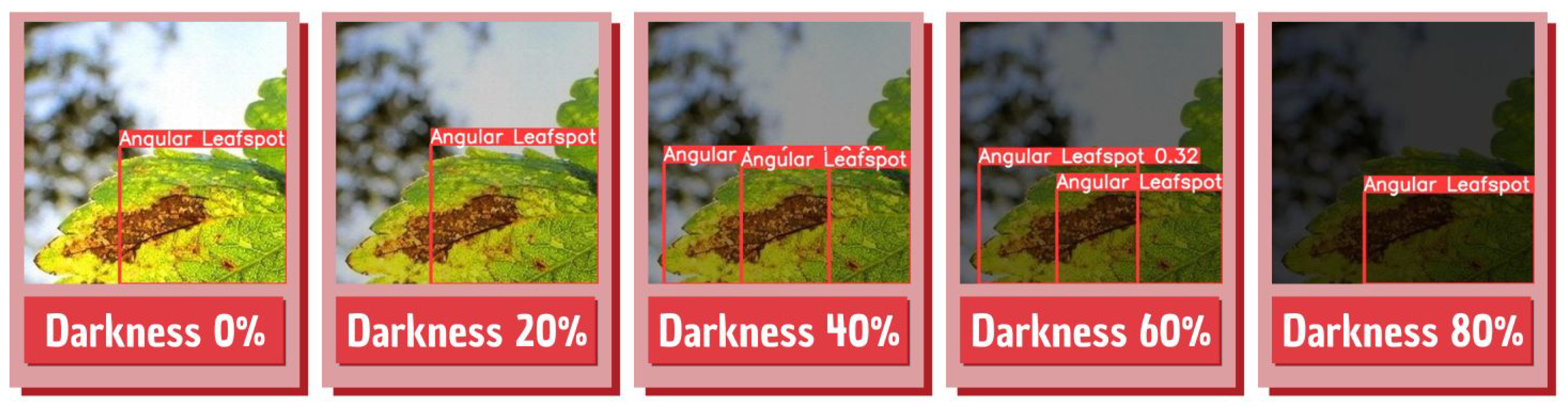
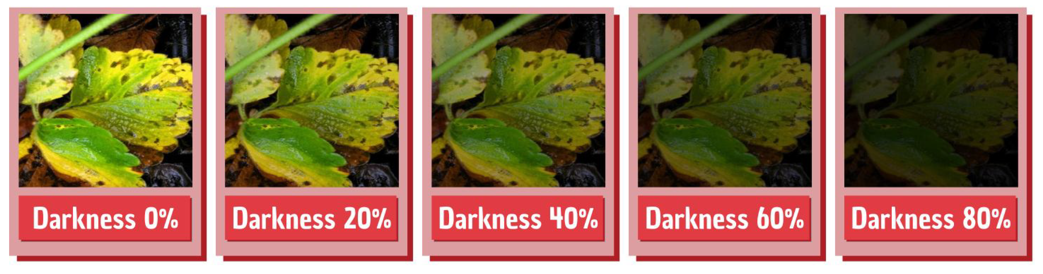
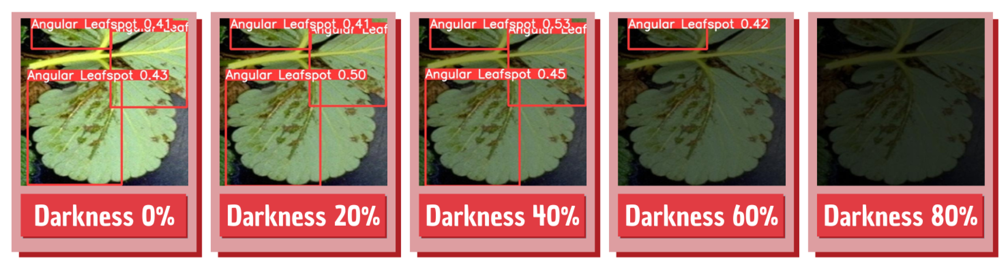
| Darkness Level | mAP 0.5 | mAP 0.5:0.95 | Precision | Accuracy | Recall |
|---|---|---|---|---|---|
| 0% | 0.9369 | 0.675 | 0.869 | 0.9112 | 0.951 |
| 20% | 0.9324 | 0.762 | 0.919 | 0.9074 | 0.9178 |
| 40% | 0.8915 | 0.727 | 0.872 | 0.8621 | 0.8562 |
| 60% | 0.6256 | 0.623 | 0.697 | 0.6517 | 0.6515 |
| 80% | 0.2582 | 0.202 | 0.351 | 0.3954 | 0.3174 |
Publisher’s Note: MDPI stays neutral with regard to jurisdictional claims in published maps and institutional affiliations. |
© 2022 by the authors. Licensee MDPI, Basel, Switzerland. This article is an open access article distributed under the terms and conditions of the Creative Commons Attribution (CC BY) license (https://creativecommons.org/licenses/by/4.0/).
Share and Cite
Cruz, M.; Mafra, S.; Teixeira, E.; Figueiredo, F. Smart Strawberry Farming Using Edge Computing and IoT. Sensors 2022, 22, 5866. https://doi.org/10.3390/s22155866
Cruz M, Mafra S, Teixeira E, Figueiredo F. Smart Strawberry Farming Using Edge Computing and IoT. Sensors. 2022; 22(15):5866. https://doi.org/10.3390/s22155866
Chicago/Turabian StyleCruz, Mateus, Samuel Mafra, Eduardo Teixeira, and Felipe Figueiredo. 2022. "Smart Strawberry Farming Using Edge Computing and IoT" Sensors 22, no. 15: 5866. https://doi.org/10.3390/s22155866
APA StyleCruz, M., Mafra, S., Teixeira, E., & Figueiredo, F. (2022). Smart Strawberry Farming Using Edge Computing and IoT. Sensors, 22(15), 5866. https://doi.org/10.3390/s22155866