Estimation of Soluble Solids for Stone Fruit Varieties Based on Near-Infrared Spectra Using Machine Learning Techniques


Abstract
:1. Introduction
2. Materials and Methods
2.1. Samples
2.2. Hardware
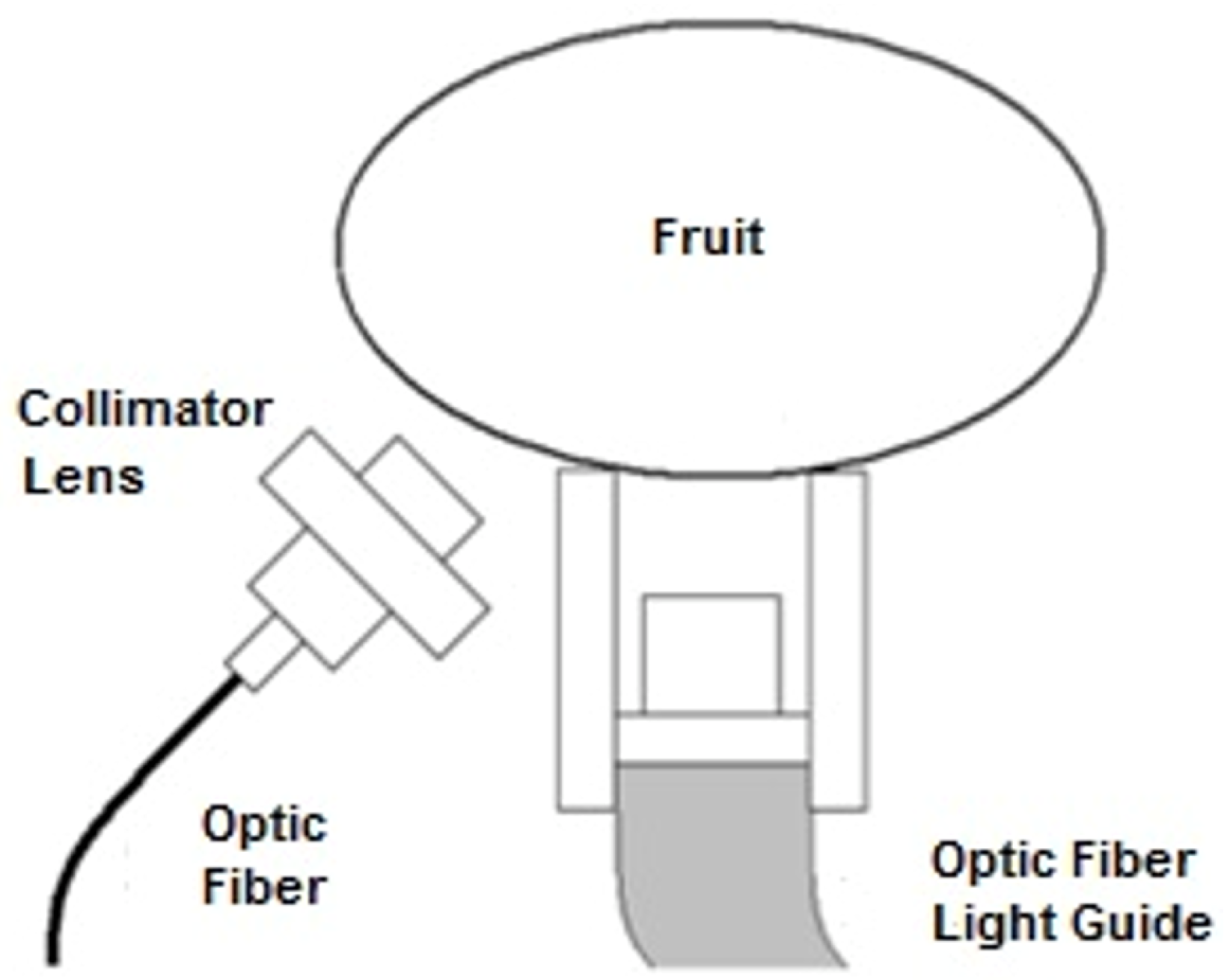
2.3. Optical Design
2.4. Acquisition
2.5. Spectral Processing
2.5.1. Spectral Correction
2.5.2. Smoothing
2.6. Convolutional Neural Network (CNN)
2.6.1. Convolutional Layer
2.6.2. Batch Normalization Layer
2.6.3. ReLU layer
2.6.4. Pooling Layer
2.6.5. Fully Connected Layer
2.6.6. Softmax Layer
2.7. Feedforward Neural Netwok (FNN)
2.8. Model Training Parameters
2.9. Model Performance Evaluation
3. Results and Discussion
4. Conclusions
Author Contributions
Funding
Institutional Review Board Statement
Informed Consent Statement
Data Availability Statement
Acknowledgments
Conflicts of Interest
Abbreviations
| VIS | Visible |
| NIR | Near Infrared |
| SS | Soluble Solids |
| CNN | Convolutional Neural Network |
| FNN | Feedforward Neural Network |
| ResNet | Residual Network |
| TP | True Positive |
| Total number of samples | |
| RMSE | Root Mean Square error |
| RMSEC | Root Mean Square Error of Calibration set |
| RMSEV | Root Mean Square Error of Validation set |
| RMSET | Root Mean Square Error of test set |
| R | Correlation Coefficient |
| Correlation Coefficient of Calibration set | |
| Correlation Coefficient of Validation set | |
| Correlation Coefficient of test set | |
| PL | Plumcot |
| PE | Peaches |
| BP | Black Plums |
| RP | Red Plums |
| WPN | White pulp nectarines |
| YPN | Yellow pulp nectarines |
References
- Crisosto, C.H.; Garner, D.; Crisosto, G.M.; Bowerman, E. Increasing ‘Blackamber’ plum (Prunus salicina Lindell) consumer acceptance. Postharvest Biol. Technol. 2004, 34, 237–244. [Google Scholar] [CrossRef]
- Crisosto, C.H.; Crisosto, G.M.; Echeverria, G.; Puy, J. Segregation of peach and nectarine (Prunus persica (L.) Batsch) cultivars according to their organoleptic characteristics. Postharvest Biol. Technol. 2006, 39, 10–18. [Google Scholar] [CrossRef]
- Crisosto, C.H.; Crisosto, G.M.; Echeverria, G.; Puy, J. Segregation of plum and pluot cultivars according to their organoleptic characteristics. Postharvest Biol. Technol. 2007, 44, 271–276. [Google Scholar] [CrossRef]
- Crisosto, C.; Valero, D. Harvesting and Postharvest Handling of Peaches for the Fresh Market; Layne, D., Bassi, D., Eds.; CABI: New York, NY, USA, 2008. [Google Scholar] [CrossRef]
- Roselló, G.R.; Montserrat, R.; Rocas, J.B. Innovación varietal en nectarina y melocotón plano o paraguayo. Rev. Frutic. 2010, 9, 4–17. [Google Scholar]
- Crisosto, C.H. Stone fruit maturity indices: A descriptive review. Postharvest News Inf. 1994, 5, 65N–68N. [Google Scholar]
- Nicolaï, B.M.; Beullens, K.; Bobelyn, E.; Peirs, A.; Saeys, W.; Theron, K.I.; Lammertyn, J. Nondestructive measurement of fruit and vegetable quality by means of NIR spectroscopy: A review. Postharvest Biol. Technol. 2007, 46, 99–118. [Google Scholar] [CrossRef]
- Chang, Y.T.; Hsueh, M.C.; Hung, S.P.; Lu, J.M.; Peng, J.H.; Chen, S.F. Prediction of specialty coffee flavors based on near-infrared spectra using machine- and deep-learning methods. J. Sci. Food Agric. 2021, 101, 4705–4714. [Google Scholar] [CrossRef]
- Moghimi, A.; Aghkhani, M.H.; Sazegarnia, A.; Sarmad, M. Nondestructive evaluation of internal quality characteristics of kiwifruit by Vis/NIR spectroscopy. J. Hortic. Sci. 2008, 22, 113–121. Available online: http://xxx.lanl.gov/abs/https://jhs.um.ac.ir/article_25069_9215f713fd8ae06703810300a5d1ca70.pdf (accessed on 30 April 2022). [CrossRef]
- Caporaso, N.; Whitworth, M.B.; Fisk, I.D. Prediction of coffee aroma from single roasted coffee beans by hyperspectral imaging. Food Chem. 2022, 371, 131159. [Google Scholar] [CrossRef]
- Slaughter, D.C.; Crisosto, C.H. Nondestructive internal quality assessment of kiwifruit using near-infrared spectroscopy. In Seminars in Food Analysis; CHAPMAN & HALL: London, UK, 1998; Volume 3, pp. 131–140. [Google Scholar]
- Carlomagno, G.; Capozzo, L.; Attolico, G.; Distante, A. Non-destructive grading of peaches by near-infrared spectrometry. Infrared Phys. Technol. 2004, 46, 23–29. [Google Scholar] [CrossRef]
- Slaughter, D. Nondestructive determination of internal quality in peaches and nectarines. Trans. ASAE 1995, 38, 617–623. [Google Scholar] [CrossRef]
- Marcelo, M.C.A.; Soares, F.F.; Ardila, J.A.; Dias, J.C.; Pedó, R.; Kaiser, S.; Pontes, O.F.S.; Pulcinelli, C.E.; Sabin, G.P. Fast inline tobacco classification by near-infrared hyperspectral imaging and support vector machine-discriminant analysis. Anal. Methods 2019, 11, 1966–1975. [Google Scholar] [CrossRef]
- Parashar, N.; Mishra, A.; Mishra, Y. Fruits Classification and Grading Using VGG-16 Approach. In Proceedings of International Conference on Communication and Artificial Intelligence; Goyal, V., Gupta, M., Mirjalili, S., Trivedi, A., Eds.; Springer Nature: Singapore, 2022; pp. 379–387. [Google Scholar]
- Budiastra, I.W.; Punvadaria, H.K. Classification of Mango by Artificial Neural Network Based on Near Infrared Diffuse Reflectance. IFAC Proc. Vol. 2000, 33, 157–161. [Google Scholar] [CrossRef]
- Xu, R.; Zhang, L.; Ding, X.; Hou, R. Classification Modeling Method for Near-Infrared Spectroscopy of Tobacco Based on Multimodal Convolution Neural Networks. J. Anal. Methods Chem. 2020, 2020, 9652470. [Google Scholar] [CrossRef]
- Wang, D.; Tian, F.; Yang, S.X.; Zhu, Z.; Jiang, D.; Cai, B. Improved Deep CNN with Parameter Initialization for Data Analysis of Near-Infrared Spectroscopy Sensors. Sensors 2020, 20, 874. [Google Scholar] [CrossRef] [PubMed]
- Zhang, X.; Xu, J.; Yang, J.; Chen, L.; Zhou, H.; Liu, X.; Li, H.; Lin, T.; Ying, Y. Understanding the learning mechanism of convolutional neural networks in spectral analysis. Anal. Chim. Acta 2020, 1119, 41–51. [Google Scholar] [CrossRef]
- Barnes, R.J.; Dhanoa, M.S.; Lister, S.J. Standard Normal Variate Transformation and De-Trending of Near-Infrared Diffuse Reflectance Spectra. Appl. Spectrosc. 1989, 43, 772–777. [Google Scholar] [CrossRef]
- Geladi, P.; MacDougall, D.; Martens, H. Linearization and Scatter-Correction for Near-Infrared Reflectance Spectra of Meat. Appl. Spectrosc. 1985, 39, 491–500. [Google Scholar] [CrossRef]
- Shin, H.C.; Roth, H.R.; Gao, M.; Lu, L.; Xu, Z.; Nogues, I.; Yao, J.; Mollura, D.; Summers, R.M. Deep Convolutional Neural Networks for Computer-Aided Detection: CNN Architectures, Dataset Characteristics and Transfer Learning. IEEE Trans. Med Imaging 2016, 35, 1285–1298. [Google Scholar] [CrossRef]
- He, K.; Zhang, X.; Ren, S.; Sun, J. Deep residual learning for image recognition. In Proceedings of the IEEE Conference on Computer Vision and Pattern Recognition, Las Vegas, NV, USA, 27–30 June 2016; pp. 770–778. [Google Scholar]
- Paoletti, M.E.; Haut, J.M.; Fernandez-Beltran, R.; Plaza, J.; Plaza, A.J.; Pla, F. Deep pyramidal residual networks for spectral–spatial hyperspectral image classification. IEEE Trans. Geosci. Remote Sens. 2018, 57, 740–754. [Google Scholar] [CrossRef]
- Gao, H.; Yang, Y.; Yao, D.; Li, C. Hyperspectral Image Classification With Pre-Activation Residual Attention Network. IEEE Access 2019, 7, 176587–176599. [Google Scholar] [CrossRef]
- Jiang, D.; Qi, G.; Hu, G.; Mazur, N.; Zhu, Z.; Wang, D. A residual neural network based method for the classification of tobacco cultivation regions using near-infrared spectroscopy sensors. Infrared Phys. Technol. 2020, 111, 103494. [Google Scholar] [CrossRef]
- Ioffe, S.; Szegedy, C. Batch Normalization: Accelerating Deep Network Training by Reducing Internal Covariate Shift. In Proceedings of Machine Learning Research, Proceedings of the 32nd International Conference on Machine Learning, Lille, France, 7–9 July 2015; Bach, F., Blei, D., Eds.; PMLR: Lille, France, 2015; Volume 37, pp. 448–456. [Google Scholar]
- Nair, V.; Hinton, G.E. Rectified Linear Units Improve Restricted Boltzmann Machines. In Proceedings of the International Conference on Machine Learning, Haifa, Israel, 21–24 June 2010. [Google Scholar]
- Gu, J.; Wang, Z.; Kuen, J.; Ma, L.; Shahroudy, A.; Shuai, B.; Liu, T.; Wang, X.; Wang, G.; Cai, J.; et al. Recent advances in convolutional neural networks. Pattern Recognit. 2018, 77, 354–377. [Google Scholar] [CrossRef]
- Wang, F.; Cheng, J.; Liu, W.; Liu, H. Additive Margin Softmax for Face Verification. IEEE Signal Process. Lett. 2018, 25, 926–930. [Google Scholar] [CrossRef]


| Fruit Species | Variety | Number of Samples |
|---|---|---|
| Peaches | Beauty Sweet | 40 |
| Elegant Lady | 60 | |
| September Sun | 60 | |
| Zee Lady | 20 | |
| Yellow Pulp Nectarines | Ruby Diamond | 20 |
| Summer Diamond | 40 | |
| Red Jim | 100 | |
| Zee Glo | 60 | |
| Venus | 60 | |
| August Red | 80 | |
| White Pulp Nectarines | Arctic Snow | 60 |
| August Pearl | 140 | |
| Giant Pearl | 140 | |
| Red Plums | Fortune | 80 |
| Red Heart | 100 | |
| Black Plums | Angeleno | 80 |
| Autumn Pride | 120 | |
| Black Kat | 120 | |
| Plumcots | Blue Gusto | 120 |
| Dapple Dandy | 80 | |
| Flavor Granade | 120 | |
| Flavor Rich | 80 |
| Min. | Max | Mean | Std. Dev. | |
|---|---|---|---|---|
| Soluble Solids Concentration (%) | 6.3 | 20.9 | 12.29 | 2.57 |
| Model | Layer | Parameters |
|---|---|---|
| CNN | Convolution 1 | Filter Size: 7 Number Filters: 64 |
| BatchNorm 1 | Mean Decay: 0.1 Variance Decay: 0.1 Epsilon: 0.00001 | |
| Max Pooling | Pool Size: 5 Stride: 1 | |
| Convolution 2 | Filter Size: 3 Number Filters: 64 | |
| BatchNorm 2 | Mean Decay: 0.1 Variance Decay: 0.1 Epsilon: 0.00001 | |
| Convolution 3 | Filter Size: 3 Number Filters: 64 | |
| BatchNorm 3 | Mean Decay: 0.1 Variance Decay: 0.1; Epsilon: 0.00001 | |
| Average Pooling | Pool Size: 5 Stride: 1 | |
| Fully Connected | Output Size: 6 | |
| Training Algorithm: Stochastic gradient descent with momentum (SGDM) | ||
| Learning Rate: 0.0001; Epochs: 200 | ||
| FNN | Hidden | Neurons: 50 |
| Training Algorithm: Scaled Conjugate Gradient | ||
| Epochs: 200 | ||
| Model | RMSEC | RMSEV | RMSET | |||
|---|---|---|---|---|---|---|
| RP | 0.6303 | 0.7054 | 0.5823 | 0.9206 | 0.8693 | 0.9548 |
| BP | 0.7345 | 0.6707 | 0.6444 | 0.9106 | 0.9171 | 0.9363 |
| PE | 1.0935 | 0.9225 | 1.1739 | 0.8408 | 0.9027 | 0.8033 |
| YPN | 1.8634 | 1.5861 | 1.9085 | 0.7109 | 0.7448 | 0.6681 |
| WPN | 1.3519 | 0.9225 | 1.1625 | 0.8981 | 0.9533 | 0.9306 |
| PL | 1.2688 | 0.8454 | 1.0859 | 0.8693 | 0.9407 | 0.9123 |
| All | 1.4108 | 1.4384 | 1.4650 | 0.8340 | 0.8258 | 0.8237 |
Publisher’s Note: MDPI stays neutral with regard to jurisdictional claims in published maps and institutional affiliations. |
© 2022 by the authors. Licensee MDPI, Basel, Switzerland. This article is an open access article distributed under the terms and conditions of the Creative Commons Attribution (CC BY) license (https://creativecommons.org/licenses/by/4.0/).
Share and Cite
Escárate, P.; Farias, G.; Naranjo, P.; Zoffoli, J.P. Estimation of Soluble Solids for Stone Fruit Varieties Based on Near-Infrared Spectra Using Machine Learning Techniques. Sensors 2022, 22, 6081. https://doi.org/10.3390/s22166081
Escárate P, Farias G, Naranjo P, Zoffoli JP. Estimation of Soluble Solids for Stone Fruit Varieties Based on Near-Infrared Spectra Using Machine Learning Techniques. Sensors. 2022; 22(16):6081. https://doi.org/10.3390/s22166081
Chicago/Turabian StyleEscárate, Pedro, Gonzalo Farias, Paulina Naranjo, and Juan Pablo Zoffoli. 2022. "Estimation of Soluble Solids for Stone Fruit Varieties Based on Near-Infrared Spectra Using Machine Learning Techniques" Sensors 22, no. 16: 6081. https://doi.org/10.3390/s22166081
APA StyleEscárate, P., Farias, G., Naranjo, P., & Zoffoli, J. P. (2022). Estimation of Soluble Solids for Stone Fruit Varieties Based on Near-Infrared Spectra Using Machine Learning Techniques. Sensors, 22(16), 6081. https://doi.org/10.3390/s22166081