1. Introduction
First developed in the 1940s, artificial neural networks have had a checkered history, sometimes lauded by researchers for their unique computational powers and other times discounted for being no better than statistical methods. About a decade ago, the power of deep artificial neural networks radically changed the direction of machine learning and rapidly made significant inroads into many scientific, medical, and engineering areas [
1,
2,
3,
4,
5,
6,
7,
8]. The strength of deep learners is demonstrated by the many successes achieved by one of the most famous and robust deep learning architectures, Convolutional Neural Networks (CNNs). CNNs frequently win image recognition competitions and have consistently outperformed other classifiers on a variety of applications, including image classification [
9,
10], object detection [
11,
12], face recognition [
13,
14], and machine translation [
15], to name a few. Not only do CNNs continue to perform better than traditional classifiers, but they also outperform human beings, including experts, in many image recognition tasks. In the medical domain, for example, CNNs have been shown to outperform human experts in recognizing skin cancer [
16], skin lesions on the face and scalp [
17], and the detection of esophageal cancer [
18].
It is no wonder, then, that CNNs and other deep learners have exploded exponentially in medical imaging research [
19]. CNNs have been successfully applied to a wide range of applications (as evidenced by these very recent reviews and studies): the identification and recognition of facial phenotypes of genetic disorders [
20], diabetic retinopathy [
21,
22,
23], glaucoma [
24], lung cancer [
25], breast cancer [
26], colon cancer [
27], gastric cancer [
28,
29], ovarian cancer [
30,
31,
32], Alzheimer’s disease [
33,
34], skin cancer [
16], skin lesions [
17], oral cancer [
35,
36], esophageal cancer [
18], and GI ulcers [
37].
Despite these successes, the unique characteristics of medical images pose challenges for CNN classification. The first challenge concerns the image size of medical data. Typical CNN image inputs are around 200 × 200 pixels. Many medical images are gigantic. For instance, histopathology slides, once digitized, often result in gigapixel images, around 100,000 × 100,000 pixels [
38]. Another problem for CNNs is the small sample size of many medical data sets. As is well known, CNNs require massive numbers of samples to prevent overfitting. It is too cumbersome, labor-intensive, and expensive to acquire collections of images numbering in the hundreds of thousands in some medical areas. There are well-known techniques for tackling the problem of overfitting when data are low, the two most common being transfer learning with pre-trained CNNs and data argumentation. The medical literature is replete with studies using both methods (for some literature reviews on these two methods in medical imaging, see [
39,
40,
41]). As observed in [
40], transfer learning works well combined with data augmentation. Transfer learning is typically applied in two ways: for fine-tuning with pre-trained CNNs and as feature extractors, with the features then fed into more traditional classifiers.
Building Deep CNN ensembles of pre-trained CNNs is yet another powerful technique for enhancing CNN performance on small sample sizes. Some examples of robust CNN ensembles reported in the last couple of years include [
42], for classifying ER status from DCE-MRI breast volumes; [
43], where a hierarchical ensemble was trained for diabetic macular edema diagnosis; [
44] for whole-brain segmentation; and [
45] for small lesion detection.
Ensemble learning combines outputs from multiple classifiers to improve performance. This method relies on the introduction of diversity, whether in the data each CNN is trained on, the type of CNNs used to build the ensemble, or some other changes in the architecture of the CNNs. For example, in [
43], mentioned above, ensembles were built on the classifier level by combining the results of two sets of CNNs within a hierarchical schema. In [
44], a novel ensemble was developed on the data level by looking at different brain areas, and in [
45], multiple-depth CNNs were trained on image patches. In [
46], CNNs with different activation functions were shown to be highly effective, and in [
47], different activation functions were inserted into different layers within a single CNN network.
In this paper, we extend [
46] by testing several activation functions with two CNNs, VGG16 [
48] and ResNet50 [
49], and their fusions across fifteen biomedical data sets representing different biomedical classification tasks. The set of activation functions includes the best-performing ones used with these networks and six new ones: 2D Mexican ReLU, TanELU, MeLU + GaLU, Symmetric MeLU, Symmetric GaLU, and Flexible MeLU. The best performance was obtained by randomly replacing every ReLU layer of each CNN with a different activation function.
The contributions of this study are the following:
- (1)
The performance of twenty individual activation functions is assessed using two CNNs (VGG16 and ResNet50) across fifteen different medical data sets.
- (2)
The performance of ensembles composed of the CNNs examined in #1 and four other topologies is evaluated.
- (3)
Six new activation functions are proposed.
The remainder of this paper is organized as follows. In
Section 2, we review the literature on activation functions used with CNNs. In
Section 3, we describe all the activation functions tested in this work. In
Section 4, the stochastic approach for constructing CNN ensembles is detailed (some other methods are described in the experimental section). In
Section 5, we present a detailed evaluation of each of the activation functions using both CNNs on the fifteen data sets, along with the results of their fusions. Finally, in
Section 6, we suggest new ideas for future investigation together with some concluding remarks.
2. Related Work with Activation Functions
Evolutions in CNN design initially focused on building better network topologies. As activation functions impact training dynamics and performance, many researchers have also focused on developing better activation functions. For many years, the sigmoid and the hyperbolic tangent were the most popular neural network activation functions. The hyperbolic tangent’s main advantage over the sigmoid is that the hyperbolic has a steeper derivative than the sigmoid function. Neither function, however, works that well with deep learners since both are subject to the vanishing gradient problem. It was soon realized that nonlinearities work better with deep learners.
One of the first nonlinearities to demonstrate improved performance with CNNs was the Rectified Linear Unit (ReLU) activation function [
50], which is equal to the identity function with positive input and zero with negative input [
51]. Although ReLU is nondifferentiable, it gave AlexNet the edge to win the 2012 ImageNet competition [
52].
The success of ReLU in AlexNet motivated researchers to investigate other nonlinearities and the desirable properties they possess. As a consequence, variations of ReLU have proliferated. For example, Leaky ReLU [
53], like ReLU, is also equivalent to the identity function for positive values but has a hyperparameter
> 0 applied to the negative inputs to ensure the gradient is never zero. As a result, Leaky ReLU is not as prone to getting caught in local minima and solves the ReLU problem with hard zeros that makes it more likely to fail to activate. The Exponential Linear Unit (ELU) [
54] is an activation function similar to Leaky ReLU. The advantage offered by ELU is that it always produces a positive gradient since it exponentially decreases to the limit point
as the input goes to minus infinity. The main disadvantage of ELU is that it saturates on the left side. Another activation function designed to handle the vanishing gradient problem is the Scaled Exponential Linear Unit (SELU) [
55]. SELU is identical to ELU except that it is multiplied by the constant
to maintain the mean and the variance of the input features.
Until 2015, activation functions were engineered to modify the weights and biases of a neural network. Parametric ReLU (PReLU) [
56] gave Leaky ReLU a learnable parameter applied to the negative slope. The success of PReLU attracted more research on the learnable activation functions topic [
57,
58]. A new generation of activation functions was then developed, one notable example being the Adaptive Piecewise Linear Unit (APLU) [
57]. APLU independently learns during the training phase the piecewise slopes and points of nondifferentiability for each neuron using gradient descent; therefore, it can imitate any piecewise linear function.
Instead of employing a learnable parameter in the definition of an activation function, as with PReLu and APLU, the construction of an activation function from a given set of functions can be learned. In [
59], for instance, it was proposed to create an activation function that automatically learned the best combinations of tanh, ReLU, and the identity function. Another activation function of this type is the S-shaped Rectified Linear Activation Unit (SReLU) [
60]. Using reinforcement learning, SReLU was designed to learn convex and nonconvex functions to imitate both the Webner–Fechner and the Stevens law. This process produced an activation called Swish, which the authors view as a smooth function that nonlinearly interpolates between the linear function and ReLU.
Similar to APLU is the Mexican ReLU (MeLU [
61]), whose shape resembles the Mexican hat wavelet. MeLU is a piecewise linear activation function that combines PReLU with many Mexican hat functions. Like APLU, MeLU has learnable parameters that approximate the same piecewise linear functions equivalent to identity when x is sufficiently large. MeLU has some main differences with respect to APLU: first, it has a much larger number of parameters; and second, the method in which the approximations are calculated for each function is different.
3. Activation Functions
As described in the Introduction, this paper explores classifying medical imagery using combinations of some of the best performing activation functions on two widely used high-performance CNN architectures: VGG16 [
48] and ResNet50 [
49], each pre-trained on ImageNet. VGG16 [
48], also known as the OxfordNet, is the second-place winner in the ILSVRC 2014 competition and was one of the deepest neural networks produced at that time. The input into VGG16 passes through stacks of convolutional layers, with filters having small receptive fields. Stacking these layers is similar in effect to CNNs having larger convolutional filters, but the stacks involve fewer parameters and are thus more efficient. ResNet50 [
49], winner of the ILSVRC 2015 contest and now a popular network, is a CNN with fifty layers known for its skip connections that sum the input of a block to its output, a technique that promotes gradient propagation and that propagates lower-level information to higher level layers.
The remainder of this section mathematically describes and discusses the twenty activation functions investigated in this study: ReLU [
50], Leaky ReLU [
62], ELU [
54], SELU [
55], PReLU [
56], APLU [
57], SReLU [
63], MeLU [
61], Splash [
64], Mish [
65], PDELU [
66], Swish [
60], Soft Learnable [
67], SRS [
67], and GaLU ([
68]), as well as the novel activation functions proposed here: 2D Mexican ReLU; TanELU; MeLU + GaLU; Symmetric MeLU; Symmetric GaLU; Flexible MeLU.
The main advantage of these more complex activation functions with learnable parameters is that they can better learn the abstract features through nonlinear transformations. This is a generic characteristic of learnable activation functions, well known in shallow networks [
69]. The main disadvantage is that activation functions with several learnable parameters need large data sets for training.
A further rationale for our proposed activation functions is to create activation functions that are quite different from each other to improve performance in ensembles; for this reason, we have developed the 2D MeLU, which is quite different from standard activation functions.
3.1. Rectified Activation Functions
3.1.1. ReLU
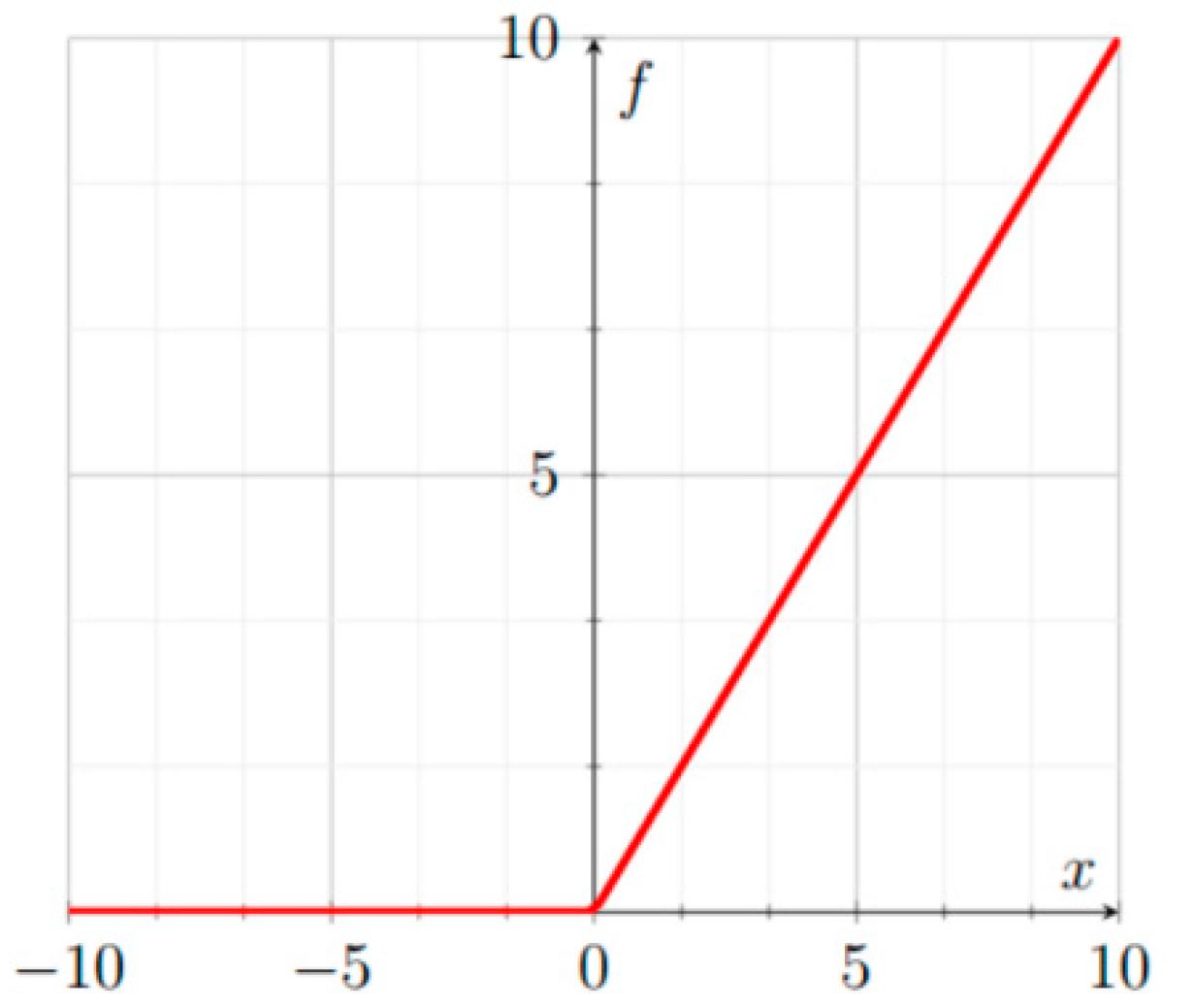
ReLU [
50], illustrated in
Figure 1, is defined as:
3.1.2. Leaky ReLU
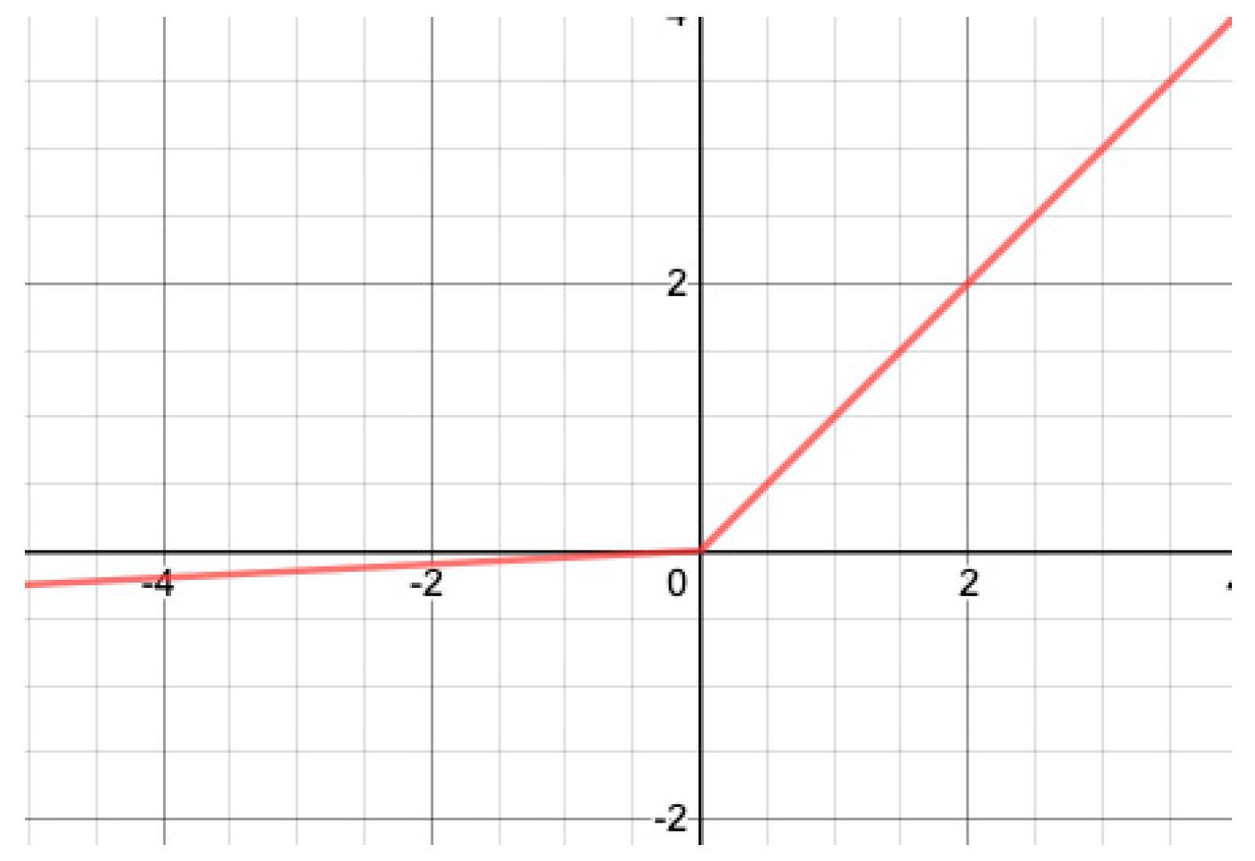
In contrast to ReLU, Leaky ReLU [
53] has no point with a null gradient. Leaky ReLU, illustrated in
Figure 2, is defined as:
where
here) is a small real number.
The gradient of Leaky ReLU is:
3.1.3. PReLU
Parametric ReLU (PreLU) [
56] is identical to Leaky ReLU except that the parameter a
c (different for every channel of the input) is learnable. PReLU is defined as:
where
is a real number.
The gradients of PReLU are:
Slopes on the left-hand sides are all initialized to 0.
3.2. Exponential Activation Functions
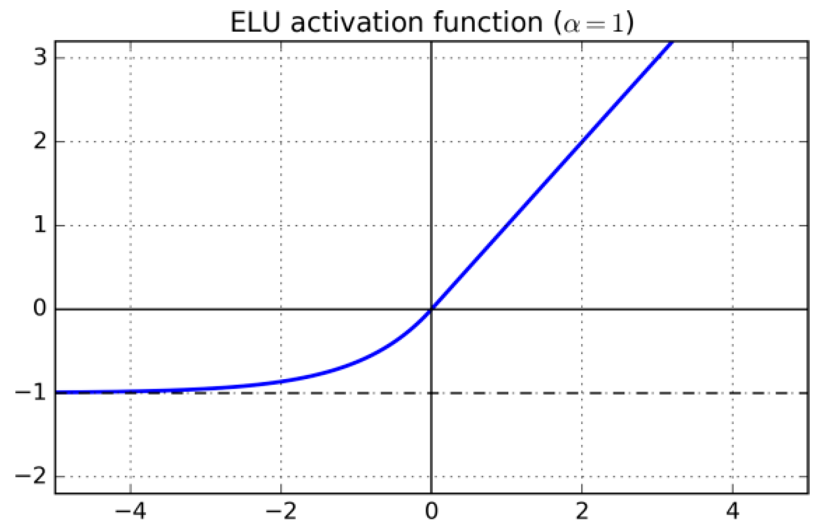
3.2.1. ELU
Exponential Linear Unit (ELU) [
54] is differentiable and, as is the case with Leaky ReLU, the gradient is always positive and bounded from below by
. ELU, illustrated in
Figure 3, is defined as:
where
here) is a real number.
The gradient of Leaky ELU is:
3.2.2. PDELU
Piecewise linear Parametric Deformable Exponential Linear Unit (PDELU) [
66] is designed to have zero mean, which speeds up the training process. PDELU is defined as
where
. The
function takes values in the
range; its slope in the negative part is controlled by means of the
parameters (
runs over the input channels) that are jointly learned by the loss function. The parameter
controls the degree of deformation of the exponential function. If
then
decays to 0 faster than the exponential.
3.3. Logistic Sigmoid and Tanh-Based AFs
3.3.1. Swish
Swish [
60] is designed using reinforcement learning to learn to efficiently sum, multiply, and compose different functions that are used as building blocks. The best function is
where
acts as a constant or a learnable parameter that is evaluated during training. When
, as in this study, Swish is equivalent to the Sigmoid-weighted Linear Unit (SiLU), proposed for reinforcement learning. As
, Swish assumes the shape of a ReLU function. Unlike ReLU, however, Swish is smooth and nonmonotonic, as demonstrated in [
60]; this is a peculiar aspect of this activation function. In practice, a value of
is a good starting point, from which performance can be further improved by training such a parameter.
3.3.2. Mish
Mish [
65] is defined as
where
is a learnable parameter.
3.3.3. TanELU (New)
TanELU is an activation function presented here that is simply the weighted sum of tanh and ReLU:
where
is a learnable parameter.
3.4. Learning/Adaptive Activation Functions
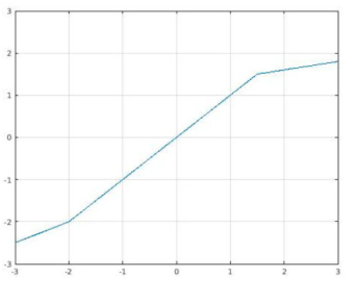
3.4.1. SReLU
S-shaped ReLU (SReLU) [
63] is composed of three piecewise linear functions expressed by four learnable parameters (
, and
initialized as
,
, a hyperparameter). This rather large set of parameters gives SReLU its high representational power. SReLU, illustrated in
Figure 4, is defined as:
where
is a real number.
The gradients of SeLU are:
Here, we use
3.4.2. APLU
Adaptive Piecewise Linear Unit (APLU) [
57] is a linear piecewise function that can approximate any continuous function on a compact set. The gradient of APLU is the sum of the gradients of ReLU and of the functions contained in the sum. APLU is defined as:
where
and
are real numbers that are different for each channel of the input.
With respect to the parameters
and
, the gradients of APLU are:
The values for
are initialized here to zero, with points randomly initialized. The 0.001
-penalty is added to the norm of the
values. This addition requires that another term
be included in the loss function:
Furthermore, a relative learning rate is added:
multiplied by the smallest value used for the rest of the network. If
is the global learning rate, then the learning rate
of the parameters
would be
3.4.3. MeLU
The mathematical basis of the Mexican ReLU (MeLU) [
61] activation function can be described as follows. Given the real numbers
and
and letting
be a so-called Mexican hat type of function, then when
, the function
is null but increases with a derivative of 1 and
between
and decreases with a derivative of
between
and
.
Considering the above, MeLU is defined as
where
is the number of learnable parameters for each channel,
are the learnable parameters, and
is the vector of parameters in PReLU.
The parameter
(
here) has one value for PReLU and
values for the coefficients in the sum of the Mexican hat functions. The real numbers
and
are fixed (see
Table 1) and are chosen recursively. The value of
is set to 256. The first Mexican hat function has its maximum at
and is equal to zero in 0 and
. The next two functions are chosen to be zero outside the interval [0,
] and [
,
], with the requirement being they have their maximum in
and
The Mexican hat functions on which MeLU is based are continuous and piecewise differentiable. Mexican hat functions are also a Hilbert basis on a compact set with the norm. As a result, MeLU can approximate every function in as k goes to infinity.
When the learnable parameters are set to zero, MeLU is identical to ReLU. Thus, MeLU can easily replace networks pre-trained with ReLU. This is not to say, of course, that MeLU cannot replace the activation functions of networks trained with Leaky ReLU and PReLU. In this study, all are initialized to zero, so start off as ReLU, with all its attendant properties.
MeLU’s hyperparameter ranges from zero to infinity, producing many desirable properties. The gradient is rarely flat, and saturation does not occur in any direction. As the size of the hyperparameter approaches infinity, it can approximate every continuous function on a compact set. Finally, the modification of any given parameter only changes the activation on a small interval and only when needed, making optimization relatively simple.
3.4.4. GaLU
Piecewise linear odd functions, composed of many linear pieces, do a better job in approximating nonlinear functions compared to ReLU [
70]. For this reason, Gaussian ReLU (GaLU) [
68], based on Gaussian types of functions, aims to add more linear pieces with respect to MeLU. Since GaLU extends MeLU, GaLU retains all the favorable properties discussed in
Section 3.4.3.
Letting
+min (
) be a Gaussian type of function, where
and
are real numbers, GaLU is defined, similarly to MeLU, as
In this work, parameters for what will be called in the experimental section Small GaLU and for GaLU proper.
Like MeLU, GaLU has the same set of fixed parameters. A comparison of values for the fixed parameters with
is provided in
Table 2.
3.4.5. SRS
Soft Root Sign (SRS) [
67] is defined as
where α and β are nonnegative learnable parameters. The output has zero means if the input is a standard normal.
3.4.6. Soft Learnable
It is defined as
where α and β are nonnegative trainable parameters that enable SRS to adaptively adjust its output to provide a zero-mean property for enhanced generalization and training speed. SRS also has two more advantages over the commonly used ReLU function: (i) it has nonzero derivative in the negative portion of the function, and (ii) bounded output, i.e., the function takes values in the range
, which is in turn controlled by the α and β parameters
We used two different versions of this activation, depending on whether the parameter is fixed (labeled here as Soft Learnable) or not (labeled here as Soft Learnable2).
3.4.7. Splash
Splash [
64] is another modification of APLU that makes the function symmetric. In the definition of APLU, let
and
be the learnable parameters leading to
. Then, Splash is defined as
This equation’s hinges are symmetric with respect to the origin. The authors in [
65] claim that this network is more robust against adversarial attacks.
3.4.8. 2D MeLU (New)
The 2D Mexican ReLU (2D MeLU) is a novel activation function presented here that is not defined component-wise; instead, every output neuron depends on two input neurons. If a layer has N neurons (or channels), its output is defined as
where
.
The parameter
is a two-dimensional vector whose entries are the same as those used in MeLU. In other words,
as defined in
Table 1. Likewise,
is defined as it is for MeLU in
Table 1.
3.4.9. MeLU + GaLU (New)
MeLU + GaLU is an activation function presented here that is, as its name suggests, the weighted sum of MeLU and GaLU:
where
is a learnable parameter.
3.4.10. Symmetric MeLU (New)
Symmetric MeLU is the equivalent of MeLU, but it is symmetric like Splash. Symmetric MeLU is defined as
where the coefficients of the two MeLUs are the same. In other words, the
k coefficients of
are the same as
.
3.4.11. Symmetric GaLU (New)
Symmetric GaLU is the equivalent of symmetric MeLU but uses GaLU instead of MeLU. Symmetric GaLU is defined as
where the coefficients of the two GaLUs are the same. In other words, the
k coefficients of
are the same as
3.4.12. Flexible MeLU (New)
Flexible MeLU is a modification of MeLU where the peaks of the Mexican function are also learnable. This feature makes it more similar to APLU since its points of nondifferentiability are also learnable. Compared to MeLU, APLU has more hyperparameters.
6. Conclusions
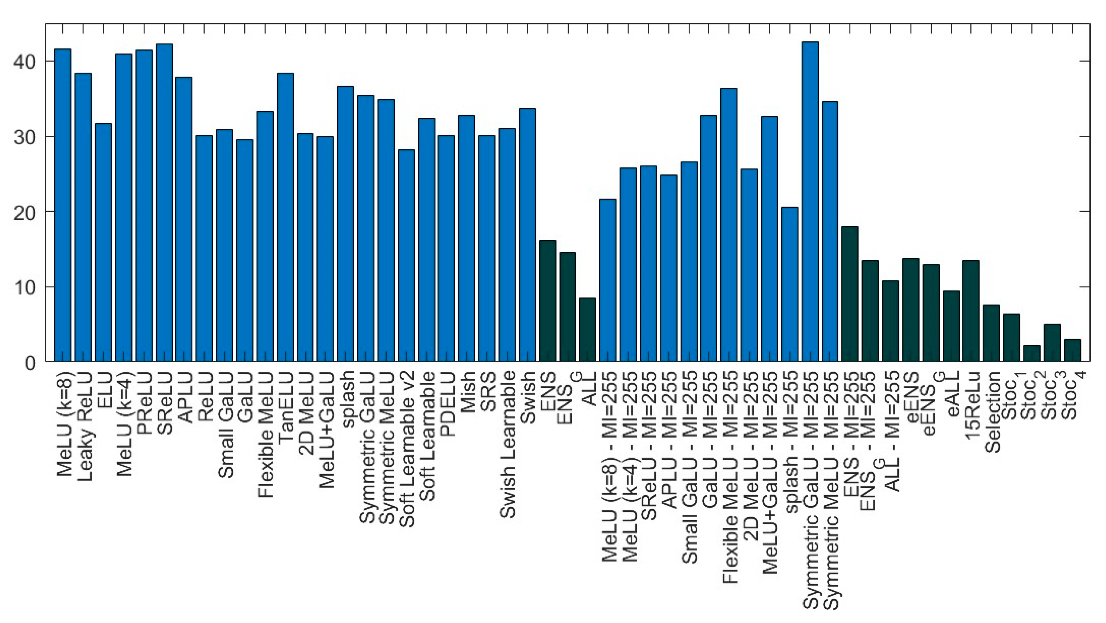
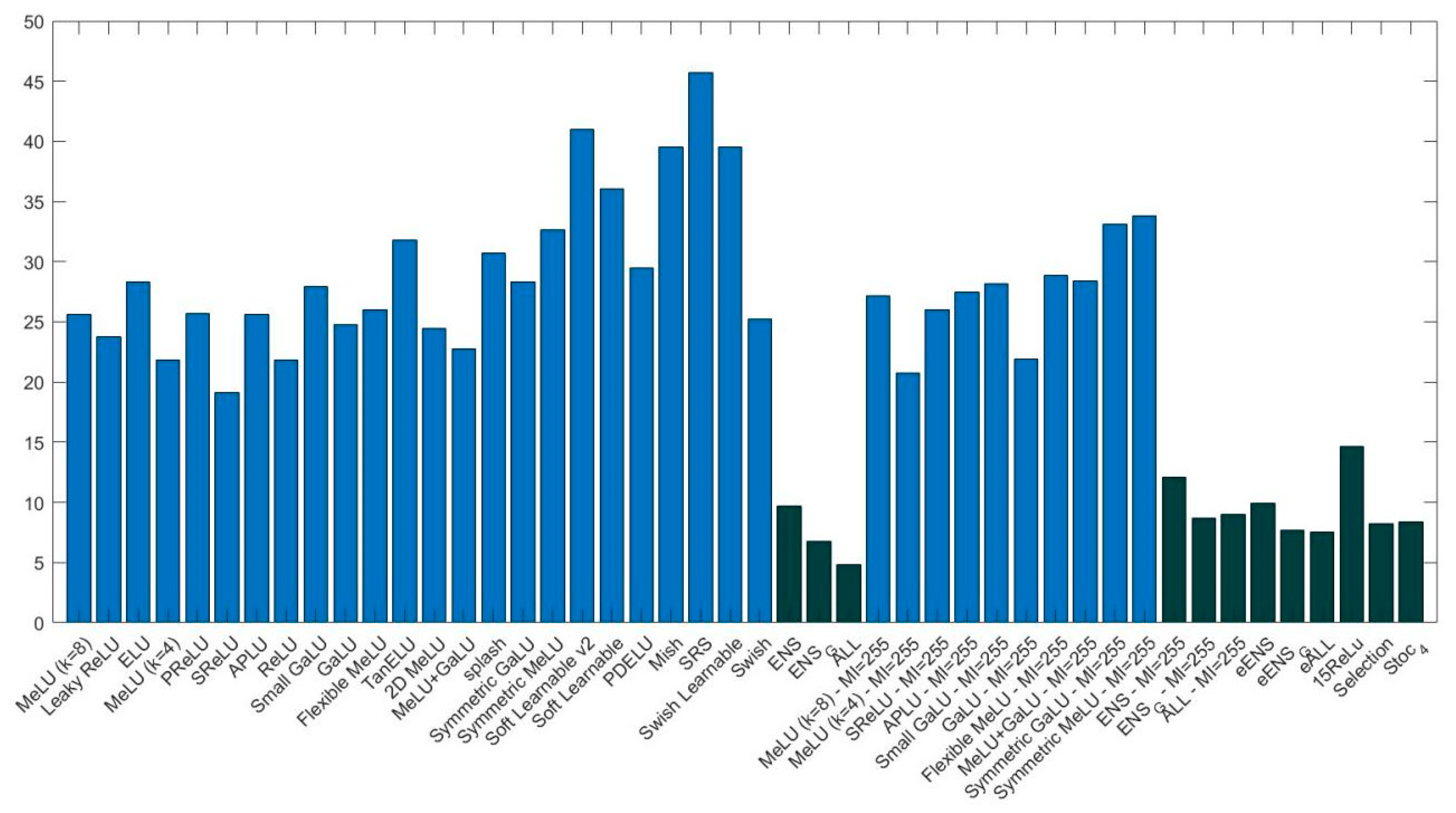
The goal of this study was to evaluate some state-of-the-art deep learning techniques on medical images and data. Towards this aim, we evaluated the performance of CNN ensembles created by replacing the ReLU layers with activations from a large set of activation functions, including six new activation functions introduced here for the first time (2D Mexican ReLU, TanELU, MeLU + GaLU, Symmetric MeLU, Symmetric GaLU, and Flexible MeLU). Tests were run on two different networks: VGG16 and ResNet50, across fifteen challenging image data sets representing various tasks. Several methods for making ensembles were also explored.
Experiments demonstrate that an ensemble of multiple CNNs that differ only in their activation functions outperforms the results of single CNNs. Experiments also show that, among the single architectures, there is no clear winner.
More studies need to investigate the performance gains offered by our approach on even more data sets. It would be of value, for instance, to examine whether the boosts in performance our system achieved on the type of data tested in this work would transfer to other types of medical data, such as Computer Tomography (CT) and Magnetic Resonance Imaging (MRI), as well as image/tumor segmentation. Studies such as the one presented here are difficult, however, because investigating CNNs requires enormous computational resources. Nonetheless, such studies are necessary to increase the capacity of deep learners to classify medical images and data accurately.


