Article

Reduction of Signal Drift in a Wavelength Modulation Spectroscopy-Based Methane Flux Sensor

by
Scott P. Seymour
,
Simon A. Festa-Bianchet
,
David R. Tyner
and
Matthew R. Johnson
*
Energy & Emissions Research Laboratory, Department of Mechanical and Aerospace Engineering, Carleton University, Ottawa, ON K1S 5B6, Canada
*
Author to whom correspondence should be addressed.
Current address: Environmental Defense Fund, Ottawa, ON K2P 0J1, Canada.
Sensors 2022, 22(16), 6139; https://doi.org/10.3390/s22166139
Submission received: 6 July 2022 / Revised: 9 August 2022 / Accepted: 12 August 2022 / Published: 17 August 2022
(This article belongs to the Section Environmental Sensing)

Abstract

:
Accurately quantifying unsteady methane venting from key oil and gas sector sources such as storage tanks and well casing vents is a critical challenge. Recently, we presented an optical sensor to meet this need that combines volume fraction and Doppler shift measurements using wavelength modulation spectroscopy with 2f harmonic detection to quantify mass flux of methane through a vent line. This paper extends the previous effort through a methodical component-by-component investigation of potential sources of thermally-induced measurement drift to guide the design of an updated sensor. Test data were analyzed using an innovative signal processing technique that permitted quantification of background wavelength modulation spectroscopy signal drift linked to specific components, and the results were successfully used to design a drift-resistant sensor. In the updated sensor, background signal strength was reduced, and stability improved, such that the empirical methane-fraction dependent velocity correction necessary in the original sensor was no longer required. The revised sensor improves previously reported measurement uncertainties on flow velocity from 0.15 to 0.10 m/s, while markedly reducing thermally-induced velocity drift from 0.44 m/s/K to 0.015 m/s/K. In the most general and challenging application, where both flow velocity and methane fraction are independently varying, the updated design reduces the methane mass flow rate uncertainty by more than a factor of six, from ±2.55 kg/h to ±0.40 kg/h. This new design also maintains the intrinsic safety of the original sensor and is ideally suited for unsteady methane vent measurements within hazardous locations typical of oil and gas facilities.

Graphical Abstract

1. Introduction

Methane (CH4) is a potent greenhouse gas with a global warming potential many times stronger than carbon dioxide (~83/30 times greater over a 20/100 year time horizon when emitted from fossil fuel sources) while also having a much shorter effective lifetime in the atmosphere (~12 years vs. hundreds of years for CO2) [1,2]. This combination means reductions in methane emission have critical immediate term benefits for slowing global temperature rise [3]. The oil and gas sector is a critical source of methane emissions and is a key focus of global methane mitigation efforts [4,5,6]. However, field measurements using a range of techniques suggest that methane emissions from the upstream oil and gas (UOG) industry are consistently higher than reported in inventories [7,8,9,10,11,12,13], and sources such as well casing gas vents and production storage tank vents may be among the most significant contributors to unreported emissions [10,14,15,16].
Part of the difficulty in accurately quantifying methane emissions from storage tanks and well casing vents has been the lack of suitable direct measurement technologies. Specific challenges include unsteady vent rates where both flow rate and methane volume fraction may vary independently; the need for large dynamic flow range, coupled with the prerequisite of near-zero backpressure to avoid affecting the emissions process (especially important for tank sources); and the stringent requirement for equipment to meet safety standards for use in hazardous locations (i.e., Class 1, Zone 0/1 explosive gas environments). Recently, Festa-Bianchet et al. [17] proposed an optical sensor capable of satisfying these requirements and providing time-resolved, point-source methane vent rate data. The system uses wavelength modulation spectroscopy (WMS), a well-known tunable diode laser absorption spectroscopy (TDLAS) technique capable of measuring volume fraction [18,19,20] and bulk flow velocity [21,22,23,24,25,26,27,28,29,30,31] based on laser absorption by a target species in an intrinsically safe design (Class 1, Zone 0/Div. 1 in Canada/the United States) that permits the system to be safely deployed in explosive atmospheres [32,33]. In controlled tests at fixed methane fractions between 25–100%, a methane flow rate uncertainty of ±0.85 kg/h was achieved. However, under varying composition scenarios, a velocity offset error was observed that depended on methane volume fraction and required implementation of a separate empirical calibration. If the methane volume fraction varied along with flow velocity, this offset correction increased the uncertainty to ±2.1 kg/h. Moreover, continued development of the system suggested velocity measurements are subject to thermally induced drift that would affect performance in varying temperature environments.
The goal of this study was to design and test an improved methane flux sensor, leveraging results of a comprehensive investigation of the sources of measurement drift. A novel experimental approach was used that directly measured the influence of individual components on changes in the background WMS signals that drive measurement drift. Compared to attempting to infer the effects of individual components from observed variability in the final measured methane volume fraction and/or velocity using the complete sensor, this method improved precision of the analysis, simplified the required experimental apparatus, and significantly accelerated testing. Ultimately this allowed a much broader range of components to be investigated and led to the design of a significantly improved methane flux sensor. More generally, this approach should be broadly useful in guiding design of other WMS sensors, regardless of the target gas and application. Experiments were performed to quantify measurement uncertainties and thermal stability of the new system and document improved performance over the initial system reported by Festa-Bianchet et al. [17]. The revised sensor is well-suited for field deployments to measure unsteady methane venting from oil and gas sector point sources within hazardous location flammable gas environments.

2. Materials and Methods
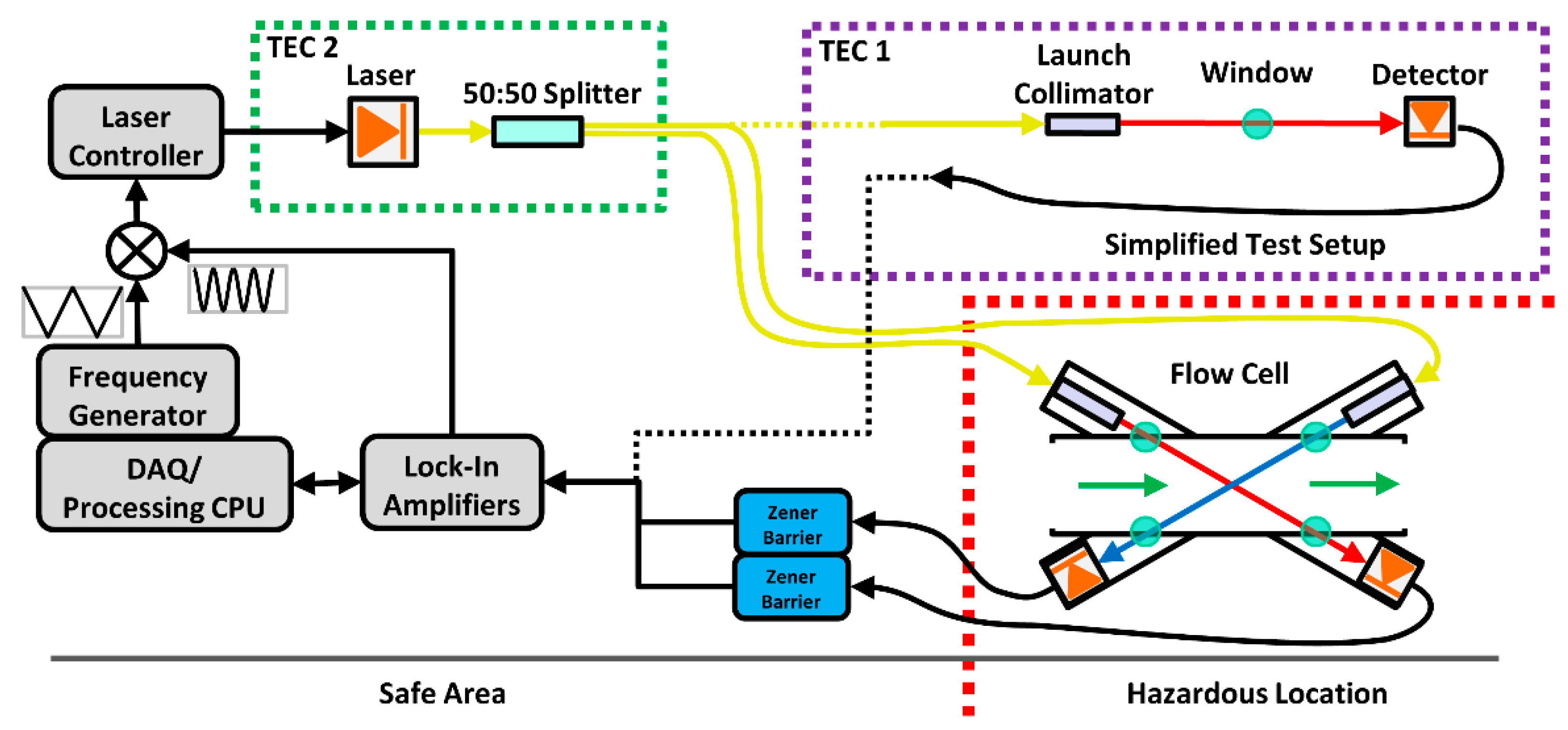
2.1. Test Apparatus

Figure 1 shows a schematic of the methane flux sensor from Festa-Bianchet et al. [17] as well as the simplified test setup used in this work to conduct thermal stability tests of specific optical components. Both systems used a distributed feedback diode laser (Eblana, EP1662-3-DM-B06-FA, Dublin, Ireland) controlled by a Stanford Research Systems laser diode controller (SRS, LDC501, Sunnyvale, CA, USA) and tuned to a center frequency of 6026.23 cm−1 (1659.41 nm) to detect the R 1 F1(1) absorption line of methane. A modulation frequency of 10 kHz with a depth of 0.1754 cm−1 (provided by a lock-in amplifier, Zurich Instruments, MFLI, Zurich, Switzerland) was superimposed on a 30 Hz triangle waveform which swept the laser’s frequency by 0.756 cm−1 (provided by a frequency generator, National Instruments, NI; PXI 5406, Austin, TX, USA) across the absorption transition line center. The modulation depth, corresponding to a modulation index m of 2.26 (where m is the ratio of modulation depth to the absorption line’s half width at half maximum), was selected to maximize the 2f response.
As in the original methane flux sensor, the laser output was coupled into single mode fiber (9/125 μm) and split equally into two beams using a fiber coupler/splitter (Thorlabs, TW1550R5A1, Newton, NJ, USA). All fiber connections used angled-physical contact (APC) connectors to minimize back-reflections. The simplified test setup differs from the original sensor by making use of only one of the splitter output fibers. This simplification was critical in reducing the number of components involved in temperature sensitivity tests, further discussed in Section 2.2.1. The single splitter output was connected to a collimator (various models) which directly irradiated a photodiode at a distance of approximately 20 cm. This spacing matched the free space distance of the original flow cell shown in the lower right of the figure. The components tested using the simplified setup were placed within a custom thermal enclosure (TEC1, see Section 2.3) which allowed the temperature to be adjusted. Similarly, for testing of the thermal stability of the laser mount and splitter, a second thermal enclosure (TEC2) was used. The photodiode signal was demodulated by the lock-in amplifier, and the harmonic outputs from the lock-in were processed in a LabVIEW environment on a host computer (NI, PXIe 8880, Austin, TX, USA).

2.2. Optical Measurement Noise and Drift

Although the WMS technique has been successfully deployed in myriad applications, performance can ultimately be limited by background WMS signals (i.e., WMS signals unrelated to the absorbing gas [34]), which are most often caused by laser speckle, etalons, and varying component transmissivity [35,36,37,38]; laser output drift [39,40]; and thermal effects of detectors [37,41,42]. These spectroscopic background signals can induce non-zero offsets in measured velocity and species volume fraction. Moreover, any time-variation in these signals can manifest as measurement drift. The methane volume fraction-dependent velocity error reported in Festa-Bianchet et al. [17] was attributed to such background signals in the 2f harmonic. Although various strategies for mitigating the impacts of background 2f noise have been investigated in the literature, including background subtraction using reference laser lines [43] or inert gas purging [44]; mechanical jitter to average out background signals [20,37]; thermal-stabilization [20]; and filtering of sinusoidal WMS signals [45], the primary strategy is always to avoid or minimize these signals as much as possible through judicious optical design and component selection. Moreover, most of these mitigation strategies are not easily applied to a field-deployable instrument.

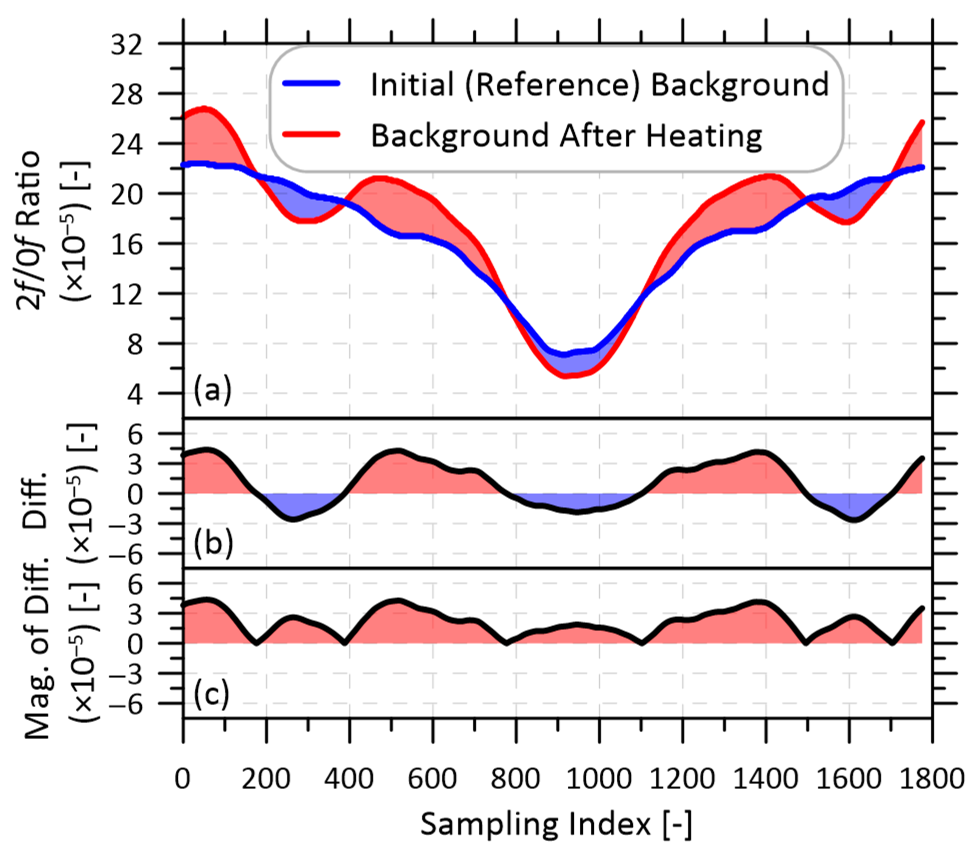
2.2.1. Quantification of Background WMS Signals

Initial efforts to quantify signal drift of the methane flow sensor focused on changes in the measured outputs of the complete optical system (i.e., volume fraction and velocity) in different configurations. However, the variable nature of signal drift and the number of required components in the fully assembled, dual-beam system made it difficult to reliably attribute changes in performance back to individual components. Moreover, longer duration stability tests required the light-absorbing gas be maintained at a stable volume fraction and flow rate. This proved difficult to achieve especially at velocities near zero where even minor temperature differences could induce convection currents on the order of 0.1 m/s.
Instead, we present a novel, simple method for quantifying changes in WMS background signals that drive overall measurement offsets and drift. This method involves recording a reference background signal (i.e., with no absorbing gas) at the beginning of the experiment, and subsequently monitoring any changes to this signal while an external disturbance, in this case a temperature change, is imposed on a subset of the system. Importantly, this approach only requires monitoring the signal from a single laser beam and it removes the need for any light-absorbing gas. This greatly simplifies the experimental setup and accelerates testing, allowing a broader range of components to be investigated as part of creating an optimized system design.
A 30-s average of a given harmonic signal was used as the reference background ( W M S r e f ) against which changes could be monitored. Changes to the background WMS signals of a test configuration ( W M S t e s t ) were evaluated based on the difference between the test and reference background signals. The absolute value of this difference, integrated across each point i of the laser sweep ( I B D ; integrated background difference), was computed as a convenient single-value parameter to characterize the change in background signals between two configurations.
I B D = i = 1 N | W M S t e s t ( i ) W M S r e f ( i ) |
Changes in I B D values among different selections and configurations of optical components were used to guide the design of a system that maximized measurement accuracy and minimized temperature-induced drift. Figure 2a shows an example of the difference between the reference 2f/0f background and the background signal after heating the components under test by 12 °C; the difference between the background signals (b) and magnitude of this difference (c) are also shown.

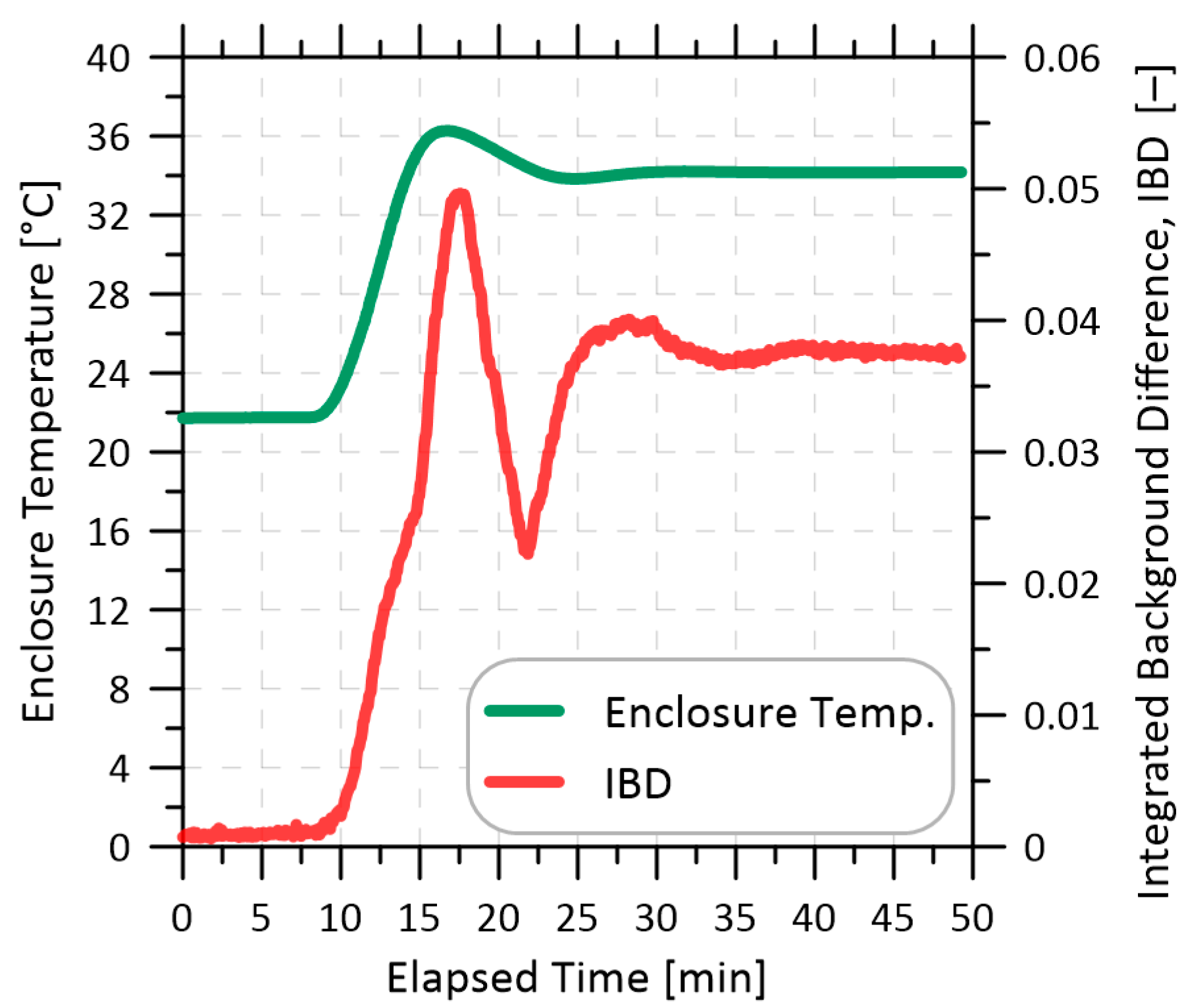
2.3. Thermal Enclosure and Component Testing Program

A custom-built thermal enclosure was used to test the temperature sensitivity of individual measurement-system components and their influence on WMS background signals as quantified via the I B D . The enclosure had an internal volume of 0.009 m3 (30 cm × 30 cm × 10 cm) and the air temperature within was controlled via a thermoelectric heater-cooler (TEC) unit (TE Technology, CP-121HT, Traverse City, MI, USA). Component(s) under test were placed within the enclosure, which was heated from 22 °C to 35 °C while the I B D was measured as illustrated in Figure 3. The initial WMS background signal at 22 °C was monitored for at least 7 min to ensure the WMS signal was stable and a 30-s average was recorded as W M S r e f . The internal temperature of the enclosure was then increased to 35 °C over a period of 10 min and maintained for at least 35 min, after which a new 30-s averaged WMS signal was recorded ( W M S t e s t ) and the I B D was calculated via Equation (1). For all component-test results presented in this work, this procedure was repeated three times. After each test, the components under test were allowed to return to 22 °C and all optical elements were reconnected and realigned to ensure that results were not specific to a particular alignment.

3. Results

3.1. Optical Component Testing

As summarized in Table 1 and Table 2, initial experiments investigated the four main components in the optical measurement path: the laser splitter (and associated connectors), launch collimator, optical windows, and photodiode detector. A summary of the test configurations is provided in Table 1 and details of the individual tested components are shown in Table 2. Comparison results, evaluated in terms of the I B D , are plotted in Figure 4.
By far the largest changes in I B D from heating, and the greatest differences among different options, were observed in the photodetector tests. Although Indium Gallium Arsenide (InGaAs) detectors are well-suited to near-infrared spectroscopic applications due to their linear response (within 0.08% uncertainty [46]) and ability to remain linear over a large power band when reverse biased [47], they can be affected by temperature near their band edges [37]. Experiments by Woodward et al. [37] showed that while the responsivity of InGaAs photodetectors is unaffected by temperature in the middle of their range (~1000–1600 nm), changes in responsivity of up to 3%/°C were measured near the band edges at 1700 nm. Interestingly, one of the worst performing photodetectors in Figure 4 is the DET1 diode used by Festa-Bianchet et al. [17], which had a manufacturer specified cut-off of 1700 nm. Interpolating the data of Woodward et al. [37] suggests that at the present measurement wavelength of 1660 nm, a change of ~0.4% per degree might be expected which may have contributed to signal drift and WMS background changes in the system of Festa-Bianchet et al. [17].
However, test results were similarly poor with an extended range InGaAs photodetector (ext-InGaAs, band edge near 1870 nm). Although initially unexpected, this result is likely due to the less uniform response of photodiodes with extended range characteristics. InGaAs photodiode spectral bands are extended to longer wavelengths by changing the ratio of Indium and Gallium in the semiconductor matrix (i.e., InxGa1−xAs); in this way, responsivity band edges can be extended to 2.5 μm [48,49,50]. Despite the shift of band edge away from the working wavelength, extended-wavelength photodiodes have also been shown to exhibit higher surface response non-uniformity and non-linearity [37,48]. This increased non-uniformity is caused by the mismatched lattice structure of the ext-InGaAs substrate which causes material strain and defects. Although improvements have been reported in ext-InGaAs manufacturing to reduce such effects [51] and small reverse biasing has been shown to improve surface uniformity [52], it was not clear from the literature how these effects would combine.
The tests in Figure 4 show that the ext-InGaAs photodetectors performed poorly (i.e., I B D was large) whether thermal stabilization was enabled (DET5-C, test configuration E) or disabled (DET5-UC, test F). The larger I B D with active diode cooling (E) is assumed to be caused by an increase in temperature swings of the photodetector case and/or its built-in window. The TEC within the photodetector moves thermal energy to the backside of the photodiode to maintain its surface temperature. However, during heating, this photodiode stabilization would introduce temperature differences between the diode surface and its case (TO-66 semiconductor package), which could affect the transmissivity or speckle pattern at the photodetector window before the beam interacts with the non-uniform surface of the photodiode [53].
The remaining three detectors (DET2, DET3, DET4) exhibited substantially lower background change when subject to the same temperature cycling. Although DET4 had the lowest mean I B D during temperature cycling ( I B D D E T 4 = 0.014), slightly below that of DET2 ( I B D D E T 2 = 0.021), the difference was not statistically significant ( p = 0.47). Moreover, use of an amplified detector (i.e., DET4) within the intended Class I, Zone 0/1 hazardous location measurement zone would require the amplification circuit to be certified as intrinsically safe. By contrast, the unamplified DET2 is considered a simple device and can be safely deployed by inserting a readily available low-resistance Zener barrier in the current loop (e.g., Pepperl + Fuchs, 937ZH-DPBN-2, Mannheim, Germany). Therefore, the unamplified DET2 photodetector (Thorlabs, SM05PD5A, Newton, NJ, USA) was selected to replace the detectors used in Festa-Bianchet et al. [17], resulting in an order of magnitude reduction in WMS background change due to the photodiode.
Although the results of Figure 4 show that the choice of launch collimator was of secondary importance, test configurations using the reflective collimators (tests B–D) had consistently lower I B D than configurations using the singlet collimators of Festa-Bianchet et al. [17]. This difference is attributed to variation in the shape and/or position of the beam striking the detector which can introduce changes to the WMS background signal due to a non-uniform photodetector surface [53]. It should be noted that mounts for the singlet and reflective collimators were also necessarily different. Some of the observed reduction in I B D may be attributable to the Polaris-K05S1 mount used with the reflective collimator, which was specifically designed to minimize deflection due to temperature changes [54]; this same mount was not directly compatible with the singlet collimator. Nevertheless, compared to the original COL2 singlet collimator assembly used by Festa-Bianchet et al. [17], the presently selected COL1 assembly produced a statistically significant reduction (p < 0.00001) in the I B D from 0.05 to 0.02 across all tests with all detectors.
In addition to collimators and photodiodes, windows are necessary in the flow cell to contain the measured gas and to separate it from the optics. Fortunately, test configurations B and J revealed no statistically significant change (p = 0.41) in I B D from inserting an angled wedged window into the optical path. Finally, results from test configuration L, which investigated heating of the laser diode assembly including the DFB laser diode, the 50:50 fiber-based splitter, and associated fiber connections, showed a mean I B D of 0.019 [-] over a 12 °C change. This I B D is similar in magnitude to that of the selected reflective collimator assembly (DET2, test configuration B) and was a statistically significant increase (p < 0.006) over a reference case (K) in which TEC2 was used to hold the temperature of these components constant. Direct heating of the individual components within the laser diode assembly using a heat gun suggested that it was specifically the FC/APC single mode fiber connections that contributed to measurement drift. Drift magnitudes were seen to increase substantially if the fiber connectors had not been properly cleaned prior to connection. All connectors were inspected by microscope and cleaned with a fiber cleaning cloth prior to final assembly. More importantly, for the final system design presented below, the laser driving components and splitter (specifically including the FC/APC connections) were temperature stabilized in a thermal enclosure (TEC2) as recommended by Schoonbaert et al. [20].

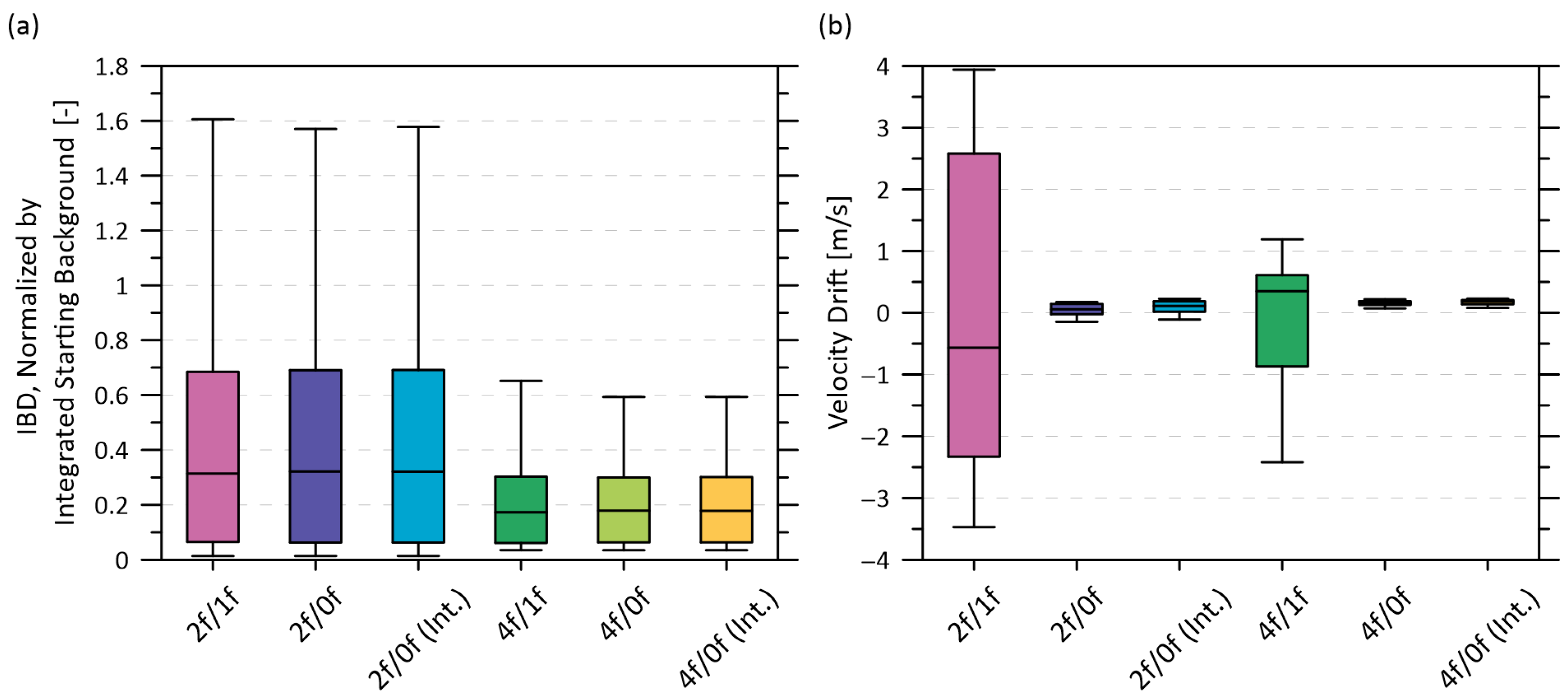
3.2. Detection Harmonic Selection

The preceding tests were all completed using 2f/0f detection. Although the 2f harmonic is the most common choice for WMS [35], the optimal harmonic is hardware-dependent and in some cases other harmonics (specifically 4f or 6f) can give greater signal-to-background ratios despite the decreased signal strength of the harmonics themselves [55]. It is also common to normalize the detection harmonic by another harmonic to remove the dependence on absolute light intensity [31,56,57]. So far in this work the 2f was divided by a linear interpolated 0f (i.e., a harmonic signal demodulated at 0 Hz to preserve only DC terms [17]). The interpolation minimizes the intensity loss due to methane absorption and is an effective estimate of the absorption free intensity, which compensates for any change in bulk transmissivity through the flow cell. However, several studies have found success using the 2f/1f harmonic ratio specifically for velocity measurements [31,38,58,59] rather than the 2f/0f. To investigate the optimal choice of detection harmonic for the present system, experiments were performed to compare the performance of six possible combinations of the 2f and 4f signals normalized by either the raw 0f signal, a linearly interpolated 0f (“0f (int.)”) signal as in [17] (i.e., where the 0f is linearly interpolated across the region of the absorption peak), or the 1f signal. Combinations using the 6f harmonic were not considered following preliminary experiments that found they had lower signal-to-background ratios than corresponding normalizations of the 4f.
Figure 5a shows box and whisker plots of I B D for each WMS harmonic, as measured during the combined experiments A–F presented in Section 3.1 using the six different detectors of Table 2. The lock-in amplifier was programmed to log four concurrent harmonics for each test: 0f, 1f, 2f, and 4f. To permit comparison given the differences in magnitude among the harmonics at the same methane absorbance, the I B D is normalized by the integrated background ( W M S r e f ) for each harmonic prior to the start of the heating cycle. From these tests, it appears that all 4f harmonic combinations experience roughly a factor of two less background change than the 2f harmonics during the heating tests. However, changes in the background signal level alone do not determine the final amount of measurement drift, particularly for velocity. The different magnitudes of the harmonics affect relative signal to noise ratios and, in particular, the different shapes of the harmonics yield different sensitivities to background noise when the up- and downstream laser signals (each with independent background optical noise characteristics) are cross-correlated to measure velocity.
To investigate this further, additional experiments were performed using the complete flow cell described in Section 3.3.1, to measure velocity drift as the entire flow cell was subjected to controlled heating (see Section 4.1). As plotted in Figure 5b, it appears that the sensitivity of the 4f to background changes offsets any benefit of the smaller I B D in Figure 5a such that measured velocity drift under temperature cycling is similar to the 2f harmonics. Moreover, these results show that the drift with 1f-normalized harmonics is worse than with either of the 0f-normalized harmonics. This was originally unexpected since previous studies [31,58] have suggested that 1f-normalized harmonics are well-suited to sensitive Doppler shift detection due to their the sharply rising shape (driven by the 1f falling toward zero at peak absorption). However, this same sharply rising 1f-normalized features is potentially more sensitive to background WMS signals at that same wavelength, especially when these backgrounds differ between the upstream and downstream laser measurement lines. The present results suggest that this sensitivity makes the 1f-normalized harmonics less stable than other harmonic combinations when the cell is subjected to thermal cycling.
Based on these results, the 2f/0f was retained as the detection signal. Although the measured velocity drift of the 4f/0f was slightly lower than that of the 2f/0f (0.15 ± 0.06 vs. 0.04 ± 0.1 m/s), the latter had superior instantaneous velocity precision (standard deviation of 0.02 m/s for 2f/0f versus 0.04 m/s for 4f/0f, both at 50% methane volume fraction). The choice of normalizing the 2f signal by either the interpolated 0f or the raw 0f signal did not have a measurable impact on velocity drift.

3.3. Improved Methane Flux Sensor

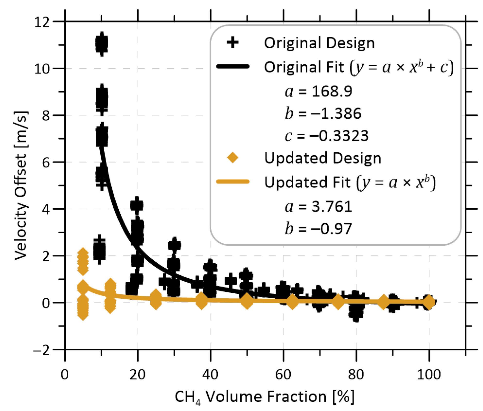
3.3.1. Updated Methane Sensor Design

The methane flow system presented in our previous work [17] was redesigned based on the preceding results. The new design used reflective collimators in Polaris mounts (COL1), unamplified photodiodes (DET2), wedged windows (WW), and stabilized the temperature of the laser driving system. Additionally, a new flow cell was constructed from Invar (an iron-nickel alloy with a low coefficient of thermal expansion, CTEInvar = ~1.2 ppm/°C) that could be compared with the original aluminum flow cell (CTEAlu = 21–24 ppm/°C). To closely match the thermal expansion of the new sensor head, the wedged windows (WW40530, Thorlabs, Newton, NJ, USA) were made of fused silica (0.55 ppm/°C) instead of N-BK7 (7.1 ppm/°C) as used in the original sensor, with a custom anti-reflective coating designed to minimize reflectance at the beam’s incidence angle. As in Festa-Bianchet et al. [17], the photodiode circuits included Zener barriers (Pepperl + Fuchs, 937ZH-DPBN-2, Mannheim, Germany) to conform to hazardous location safety requirements. A pre-computed look-up table (LUT) of coefficients was generated for the methane absorption line at 6026.23 cm1 (1659.1 nm) using spectroscopic data from HITRAN 2012 and a Lorentzian lineshape [60]. This LUT was used to calculate theoretical peak heights of the second harmonic (2f) across a range of temperatures (−30 to +70 °C, steps of 1 °C), pressures (90 to 105 kPa, steps of 2.5 kPa), and methane volume fractions (0 to 100%, steps of 1%). The calculated theoretical 2f peak heights, scaled by the estimated absorption-free intensity, were then linearly interpolated using the measured 2f peak height, gas temperature, and pressure to obtain a theoretical methane volume fraction. This methane volume fraction was then combined with intrinsically-safe measurements of temperature and pressure to calculate gas density, which was combined with the measured flow velocity to yield the methane mass flow rate. The updated flow cell is shown in Figure 6, along with its principal dimensions and components.

4. Discussion

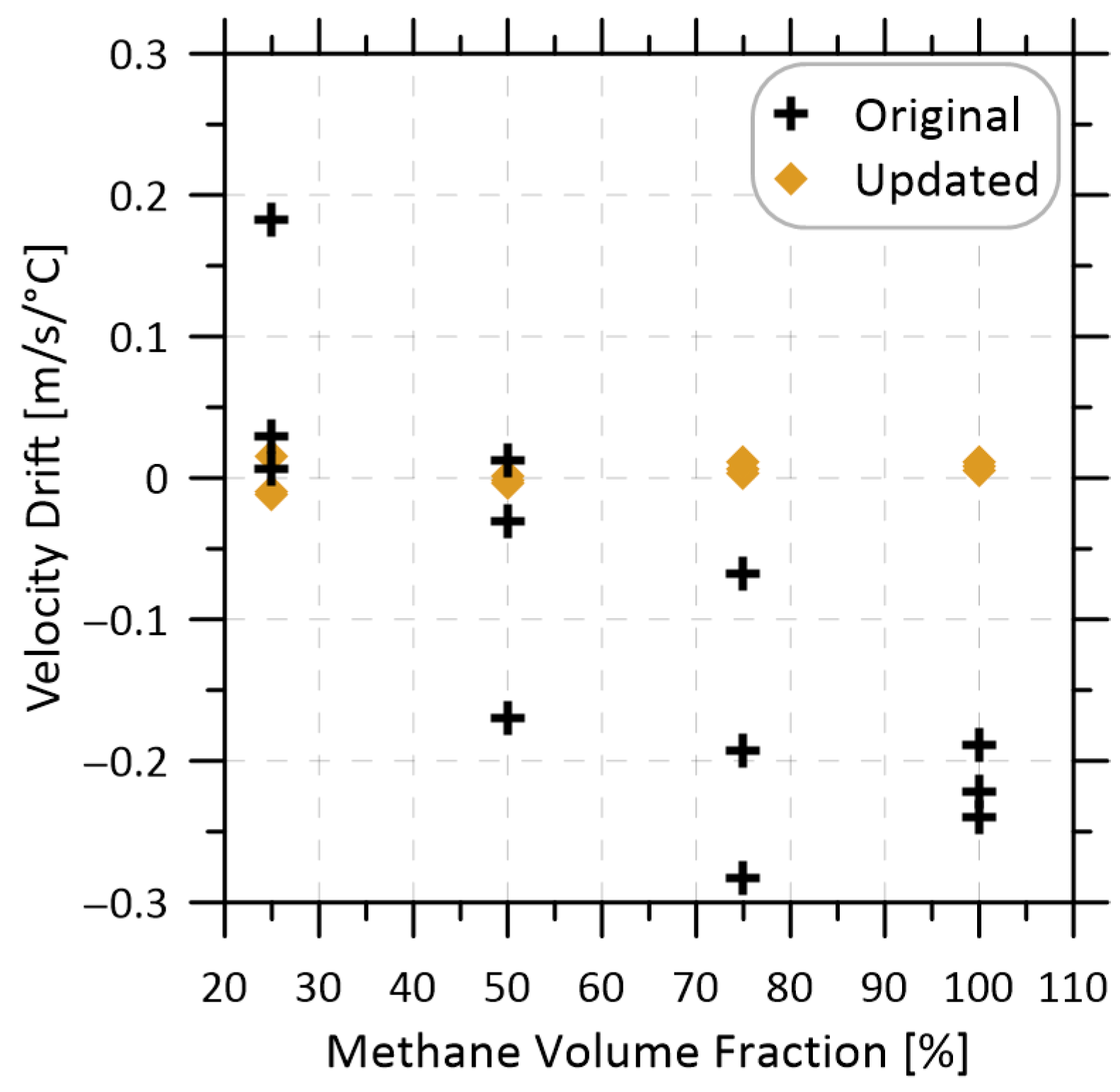
4.1. Temperature Stability of the Updated Sensor

To validate the combined improvements made to the system, two insulated enclosures large enough to contain either the original methane sensor (Original) or the new methane sensor (Updated) were constructed. Two fans and a 90 W heater within the enclosure (operated using a PID controller) raised the temperature from ambient to 37 °C (roughly a 12 °C change) over the course of 1.5 h to ensure that a stable temperature had been reached. Valves were installed on both ends of the two flow cells to seal various methane-nitrogen mixtures within the cells, such that any drift in the measurements due to temperature change could be monitored at stable methane volume fractions. Figure 7 plots the measured velocity drifts during these tests, which have been normalized by the measured temperature change to permit direct comparison.
The mean velocity drift of the updated flow cell was approximately 25 times lower than that of the original. Across three repeats at 25, 50, 75, and 100% methane, the original system had a mean drift of −0.1 ± 0.33 m/s/°C while the revised sensor had a mean drift of 0.004 ± 0.021 m/s/°C, both at 95% confidence. Interestingly, the original sensor showed an apparent negative drift correlation with methane fraction (R2 = 0.67), which may have been caused by changes to the background WMS signals [17]. By contrast, the updated sensor shows no apparent correlation of drift with methane fraction (R2 = 0.24) as further discussed below.
Although reducing the impact of background signal drift on the measured velocity was the primary focus of this study, the impact on the methane volume fraction measurement was also estimated. Since the magnitude of drift in the measured methane volume fraction was too low to be detected beyond the 0.5% precision of the instrument (see Figure 8a), the drift was instead inferred from analysis of measured changes in the background WMS signals. With each methane sensor purged with nitrogen, the background change at the 2f peak location was measured during heating of the measurement cell. The magnitude of this change was then used to calculate the maximum expected change in measured methane volume fraction, which would occur at 100% methane. Results from three repeated experiments show that the absolute methane volume fraction can be expected to vary by no more than 0.02% ± 0.06%/°C for the original system versus 0.007% ± 0.009%/°C for the updated design, both at 95% confidence.

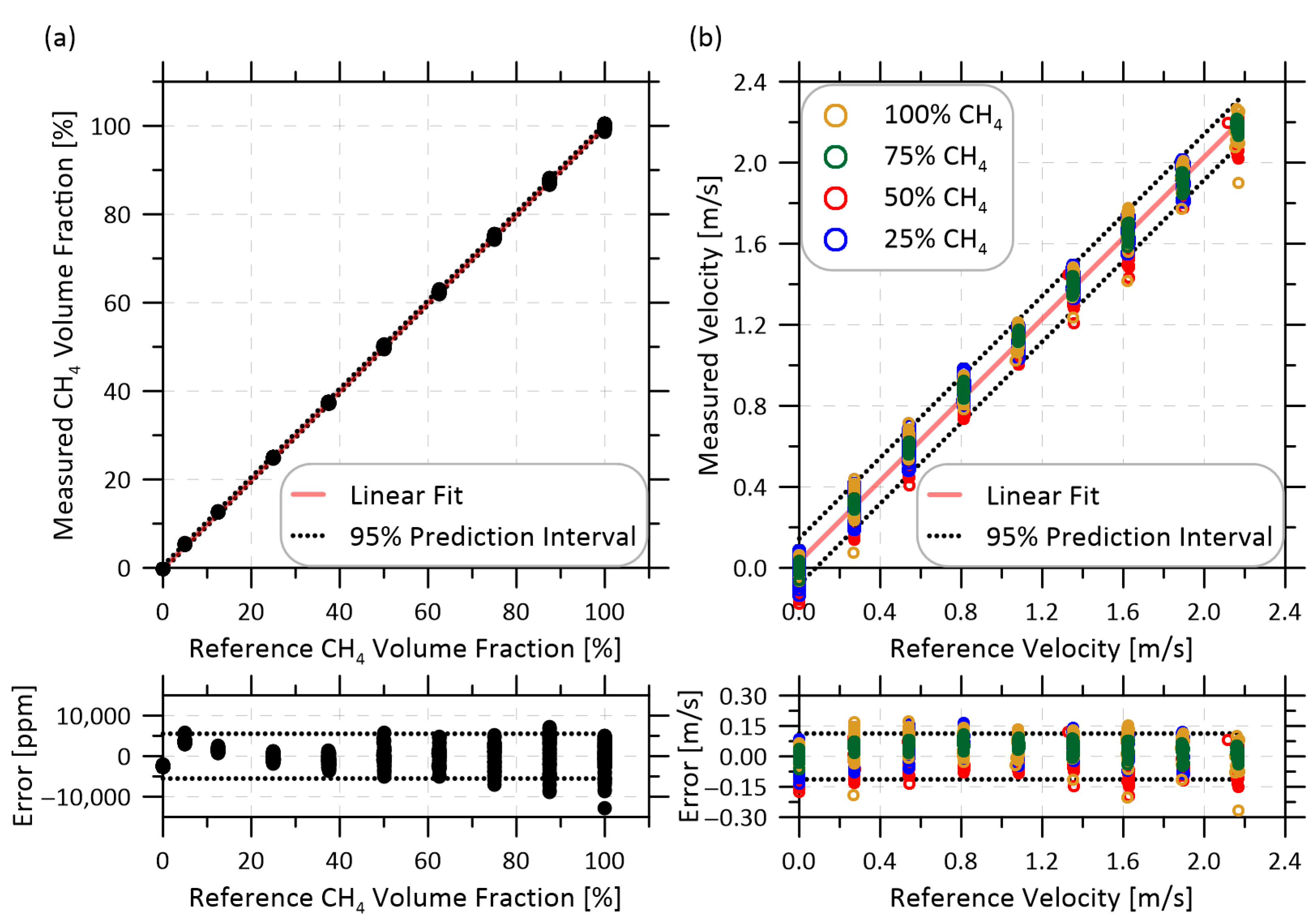
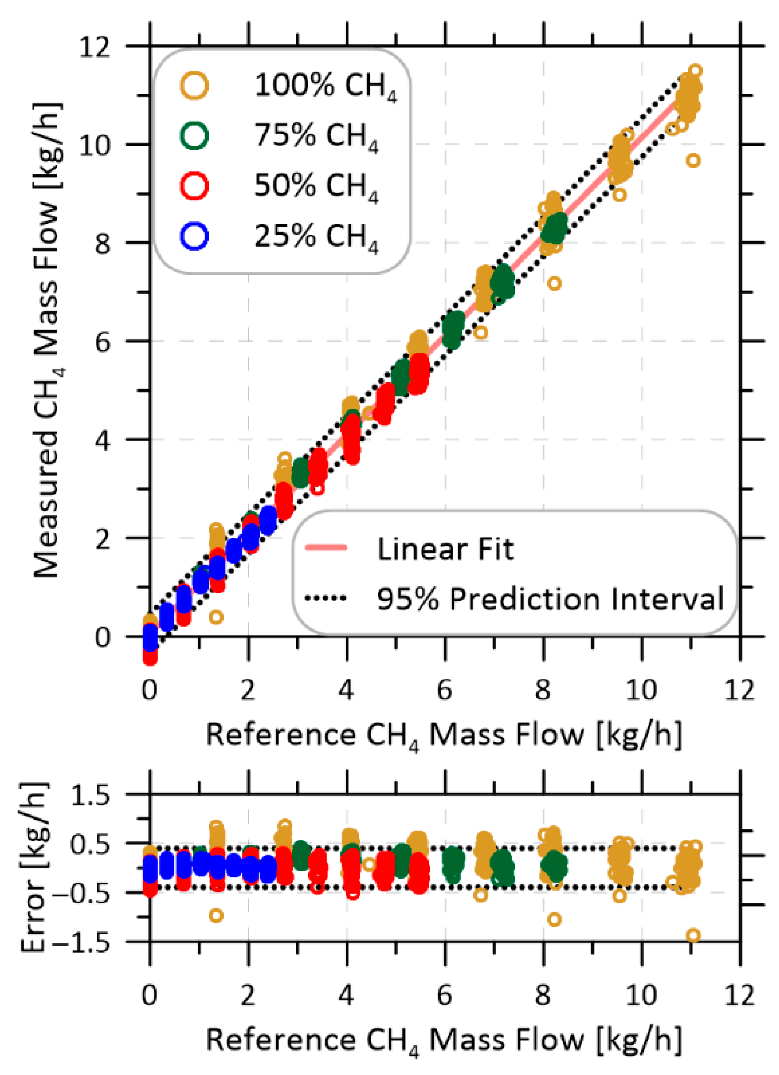
4.2. Measurement Uncertainty of the Updated Sensor

Performance testing of the updated system was completed to quantify final measurement uncertainties and any improvements over the original design. Bottled compressed methane (ME 2.0-T, 99.0% CH4, Linde Canada, Mississauga, ON, Canada) and nitrogen (NI 5.0UH-T, 99.999% N2, Linde Canada) were metered using two calibrated thermal mass flow controllers (MFCs, EL-FLOW F-202AV-M10-RAD-55-V, Bronkhorst, Ruurlo, The Netherlands) and mixed to create a range of controlled flow rates and volume mixing ratios that were directed through the optical measurement cell. Velocity and methane fraction were recorded at a sampling rate of 1 Hz. Calibration curves for methane fraction and velocity measurements (polynomial and linear, respectively, as in Festa-Bianchet et al. [17]) were derived for the updated sensor and applied to subsequent test data. Tests spanned the full range of 0 to 100% methane at velocities of up to 2.2 m/s, limited by the maximum flow rates of the MFCs. These ranges corresponded to a methane mass flow range of 0 to 11 kg/h. Experiments were repeated five times over the course of three days to assess repeatability. Figure 8 plots the combined data from all 5 tests. The dotted lines indicate prediction intervals at 95% confidence. These results demonstrate a measurement uncertainty on methane volume fraction within ±0.5% methane and velocity within ±0.1 m/s.
As previously mentioned, the original methane mass flow sensor required an empirical velocity offset correction that was dependent on methane volume fraction. This velocity offset placed a significant limitation on the applicability of the sensor, restricting its usefulness to specific scenarios where the methane volume fraction was not expected to vary. Importantly, no such correction was applied to the data for the updated sensor shown in Figure 8. To investigate this further, Figure 9 reproduces the original velocity offset data and derived correction function from Festa-Bianchet et al. [17], and overlays equivalent test data for the updated flow cell from the present work. While in both cases, the apparent velocity offset became undefined towards zero methane fraction as there is no longer a methane signal to detect, the present data demonstrate that the offset is negligible at methane fractions ≥ 25%. This is a significant improvement over the previous design.
Finally, Figure 10 plots measured methane mass flows using the updated system versus prescribed flow rates from the mass flow controllers. The different colors identify measurements made at different methane volume fractions between 25–100%. The lower plot shows the error in the measured flow rate and for both plots the dotted lines show prediction intervals at 95% confidence. Over the full range of data in Figure 10, the updated methane sensor achieved a mass flow rate uncertainty of ±0.40 kg/h at 95% confidence. This is more than a factor of six improvement over the previous sensor that reported a ±2.55 kg/h uncertainty under identical conditions, and more than a factor of two improvement over the previous best case ±0.85 kg/h uncertainty for scenarios where the methane volume fraction was stable.

4.3. Outlook

Based on the preceding results, the newly designed methane flux sensor is capable of accurate, stable, time-resolved (1 Hz) quantification of methane flows, while being safely deployable in Class I, Zone 0/1 hazardous locations due to presence of flammable gases. This makes it ideally suited for applications in the upstream oil and gas industry, where there is an urgent need for technologies to quantify unsteady methane emissions from key venting-sources such as liquid storage tanks and casing gas vents that can dominate total emissions [10,11]. As a technique for quantifying tank venting, the sensor could be used to assess tank venting models [61,62,63] as well as assumed regional compositions of the vented gas [64,65]. Coupled with tank level or other measurements of produced oil volumes, the sensor could be used to measure time-resolved gas production or casing gas venting sufficient to calculate real-time gas-oil-ratios (GOR). This could overcome a key barrier to accurate methane emissions reporting, where poorly estimated GOR has been implicated in several studies as a key reason for underestimation of venting in current inventories [11,14,66,67].

Author Contributions

Conceptualization and Methodology, S.P.S., S.A.F.-B., M.R.J. and D.R.T.; Investigation, S.P.S. and S.A.F.-B.; Formal Analysis, S.P.S. and S.A.F.-B.; Writing—Original draft, S.P.S. and M.R.J.; Writing—Review & Editing, M.R.J., S.P.S. and S.A.F.-B.; Funding Acquisition, M.R.J. and S.A.F.-B. All authors have read and agreed to the published version of the manuscript.

Funding

This work was funded by Natural Resources Canada through the Clean Growth Program (grant number CGP-17-0905), the Natural Sciences and Engineering Research Council of Canada (NSERC, grant numbers 06632 and 522658), and Mitacs (grant number IT18367). The APC was funded by NSERC.

Conflicts of Interest

The authors declare no conflict of interest.

References

  1. Joos, F.; Roth, R.; Fuglestvedt, J.S.; Peters, G.P.; Enting, I.G.; Von Bloh, W.; Brovkin, V.; Burke, E.J.; Eby, M.; Edwards, N.R.; et al. Carbon Dioxide and Climate Impulse Response Functions for the Computation of Greenhouse Gas Metrics: A Multi-Model Analysis. Atmos. Chem. Phys. 2013, 13, 2793–2825. [Google Scholar] [CrossRef]
  2. Forster, P.; Storelvmo, T.; Armour, K.; Collins, W.; Dufresne, J.-L.; Frame, D.; Lunt, D.J.; Mauritsen, T.; Palmer, M.D.; Watanabe, M.; et al. Chapter 7: The Earth’s Energy Budget, Climate Feedbacks, and Climate Sensitivity. In Climate Change 2021: The Physical Science Basis. Contribution of Working Group I to the Sixth Assessment Report of the Intergovernmental Panel on Climate Change; Masson-Delmotte, V., Zhai, P., Pirani, A., Connors, S.L., Péan, C., Berger, S., Caud, N., Chen, Y., Goldfarb, L., Gomis, M.I., et al., Eds.; Cambridge University Press: Cambridge, UK, 2021. [Google Scholar]
  3. Ocko, I.B.; Sun, T.; Shindell, D.; Oppenheimer, M.; Hristov, A.N.; Pacala, S.W.; Mauzerall, D.L.; Xu, Y.; Hamburg, S.P. Acting rapidly to deploy readily available methane mitigation measures by sector can immediately slow global warming. Environ. Res. Lett. 2021, 16, 054042. [Google Scholar] [CrossRef]
  4. IEA. Net Zero by 2050: A Roadmap for the Global Energy Sector; International Energy Agency (IEA): Paris, France, 2021. [Google Scholar]
  5. The White House Office of Domestic Climate Policy. U.S. Methane Emissions Reduction Action Plan; The White House: Washington, DC, USA, 2021. [Google Scholar]
  6. CCAC. Global Methane Pledge. Available online: https://www.globalmethanepledge.org/ (accessed on 28 April 2022).
  7. Hmiel, B.; Petrenko, V.V.; Dyonisius, M.N.; Buizert, C.; Smith, A.M.; Place, P.F.; Harth, C.; Beaudette, R.; Hua, Q.; Yang, B.; et al. Preindustrial 14CH4 Indicates Greater Anthropogenic Fossil CH4 Emissions. Nature 2020, 578, 409–412. [Google Scholar] [CrossRef] [PubMed]
  8. Alvarez, R.A.; Zavala-Araiza, D.; Lyon, D.R.; Allen, D.T.; Barkley, Z.R.; Brandt, A.R.; Davis, K.J.; Herndon, S.C.; Jacob, D.J.; Karion, A.; et al. Assessment of Methane Emissions from the U.S. Oil and Gas Supply Chain. Science 2018, 361, 186–188. [Google Scholar] [CrossRef] [PubMed]
  9. Chen, Y.; Sherwin, E.D.; Berman, E.S.F.; Jones, B.B.; Gordon, M.P.; Wetherley, E.B.; Kort, E.A.; Brandt, A.R. Quantifying Regional Methane Emissions in the New Mexico Permian Basin with a Comprehensive Aerial Survey. Environ. Sci. Technol. 2022, 56, 4317–4323. [Google Scholar] [CrossRef]
  10. Tyner, D.R.; Johnson, M.R. Where the Methane Is—Insights from Novel Airborne LiDAR Measurements Combined with Ground Survey Data. Environ. Sci. Technol. 2021, 55, 9773–9783. [Google Scholar] [CrossRef]
  11. Johnson, M.R.; Tyner, D.R.; Conley, S.A.; Schwietzke, S.; Zavala-Araiza, D. Comparisons of Airborne Measurements and Inventory Estimates of Methane Emissions in the Alberta Upstream Oil and Gas Sector. Environ. Sci. Technol. 2017, 51, 13008–13017. [Google Scholar] [CrossRef]
  12. Thompson, R.L.; Sasakawa, M.; Machida, T.; Aalto, T.; Worthy, D.; Lavric, J.V.; Myhre, C.L.; Stohl, A. Methane Fluxes in the High Northern Latitudes for 2005-2013 Estimated Using a Bayesian Atmospheric Inversion. Atmos. Chem. Phys. 2017, 17, 3553–3572. [Google Scholar] [CrossRef]
  13. Chan, E.; Worthy, D.E.J.; Chan, D.; Ishizawa, M.; Moran, M.D.; Delcloo, A.; Vogel, F. Eight-Year Estimates of Methane Emissions from Oil and Gas Operations in Western Canada Are Nearly Twice Those Reported in Inventories. Environ. Sci. Technol. 2020, 54, 14899–14909. [Google Scholar] [CrossRef]
  14. Roscioli, J.R.; Herndon, S.C.; Yacovitch, T.I.; Knighton, W.B.; Zavala-Araiza, D.; Johnson, M.R.; Tyner, D.R. Characterization of Methane Emissions from Five Cold Heavy Oil Production with Sands (CHOPS) Facilities. J. Air Waste Manag. Assoc. 2018, 68, 671–684. [Google Scholar] [CrossRef]
  15. Lavoie, T.N.; Shepson, P.B.; Cambaliza, M.O.L.; Stirm, B.H.; Conley, S.A.; Mehrotra, S.; Faloona, I.C.; Lyon, D.R. Spatiotemporal Variability of Methane Emissions at Oil and Natural Gas Operations in the Eagle Ford Basin. Environ. Sci. Technol. 2017, 51, 8001–8009. [Google Scholar] [CrossRef] [PubMed]
  16. Lyon, D.R.; Alvarez, R.A.; Zavala-Araiza, D.; Brandt, A.R.; Jackson, R.B.; Hamburg, S.P. Aerial Surveys of Elevated Hydrocarbon Emissions from Oil and Gas Production Sites. Environ. Sci. Technol. 2016, 50, 4877–4886. [Google Scholar] [CrossRef] [PubMed]
  17. Festa-Bianchet, S.A.; Seymour, S.P.; Tyner, D.R.; Johnson, M.R. A Wavelength Modulation Spectroscopy-Based Methane Flux Sensor for Quantification of Venting Sources at Oil and Gas Sites. Sensors 2022, 22, 4175. [Google Scholar] [CrossRef] [PubMed]
  18. Shemshad, J.; Aminossadati, S.M.; Kizil, M.S. A Review of Developments in near Infrared Methane Detection Based on Tunable Diode Laser. Sens. Actuators B Chem. 2012, 171–172, 77–92. [Google Scholar] [CrossRef]
  19. Norooz Oliaee, J.; Sabourin, N.A.; Festa-Bianchet, S.A.; Gupta, J.A.; Johnson, M.R.; Thomson, K.A.; Smallwood, G.J.; Lobo, P. Development of a Sub-Ppb Resolution Methane Sensor Using a GaSb-Based DFB Diode Laser near 3270 Nm for Fugitive Emission Measurement. ACS Sens. 2022, 7, 564–572. [Google Scholar] [CrossRef]
  20. Schoonbaert, S.B.; Tyner, D.R.; Johnson, M.R. Remote Ambient Methane Monitoring Using Fiber-Optically Coupled Optical Sensors. Appl. Phys. B 2015, 119, 133–142. [Google Scholar] [CrossRef]
  21. Measures, R.M. Selective Excitation Spectroscopy and Some Possible Applications. J. Appl. Phys. 1968, 39, 5232. [Google Scholar] [CrossRef]
  22. Philippe, L.C.; Hanson, R.K. Laser-Absorption Mass Flux Sensor for High-Speed Airflows. Opt. Lett. 1991, 16, 2002–2004. [Google Scholar] [CrossRef]
  23. Kurtz, J.; Wittig, S.; O’Byrne, S. Applicability of a Counterpropagating Laser Airspeed Sensor to Aircraft Flight Regimes. J. Aircr. 2016, 53, 439–450. [Google Scholar] [CrossRef]
  24. Arroyo, M.P.; Langlois, S.; Hanson, R.K. Diode-Laser Absorption Technique for Simultaneous Measurements of Multiple Gasdynamic Parameters in High-Speed Flows Containing Water Vapor. Appl. Opt. 1994, 33, 3296–3307. [Google Scholar] [CrossRef]
  25. Upschulte, B.; Miller, M.; Allen, M.G.; Jackson, K.; Gruber, M.; Mathur, T. Continuous Water Vapor Mass Flux and Temperature Measurements in a Model Scramjet Combustor Using a Diode Laser Sensor. In Proceedings of the 37th AIAA Aerospace Sciences Meeting & Exhibit, Reno, NV, USA, 11–14 January 1999; American Institute of Aeronautics and Astronautics: Reston, VI, USA, 1999. [Google Scholar]
  26. Schultz, I.A.; Goldenstein, C.S.; Jeffries, J.B.; Hanson, R.K.; Rockwell, R.D.; Goyne, C.P. Spatially Resolved Water Measurements in a Scramjet Combustor Using Diode Laser Absorption. J. Propuls. Power 2014, 30, 1551–1558. [Google Scholar] [CrossRef]
  27. Strand, C.L.; Hanson, R.K. Quantification of Supersonic Impulse Flow Conditions via High-Bandwidth Wavelength Modulation Absorption Spectroscopy. AIAA J. 2015, 53, 2978–2987. [Google Scholar] [CrossRef]
  28. Chen, S.J.; Paige, M.E.; Silver, J.A.; Williams, S.; Barhorst, T. Laser-Based Mass Flow Rate Sensor Onboard HIFiRE Flight 1. In Proceedings of the 45th AIAA/ASME/SAE/ASEE Joint Propulsion Conference & Exhibit, Denver, CO, USA, 2–5 August 2009; pp. 1–7. [Google Scholar] [CrossRef]
  29. Barhorst, T.; Williams, S.; Chen, S.J.; Paige, M.E.; Silver, J.A.; Sappey, A.; McCormick, P.; Masterson, P.; Zhao, Q.; Sutherland, L.; et al. Development of an in Flight Non-Intrusive Mass Capture System. In Proceedings of the 45th AIAA/ASME/SAE/ASEE Joint Propulsion Conference & Exhibit, Denver, CO, USA, 2–5 August 2009; pp. 1–11. [Google Scholar] [CrossRef]
  30. Lyle, K.H.; Jeffries, J.B.; Hanson, R.K. Diode-Laser Sensor for Air-Mass Flux 1: Design and Wind Tunnel Validation. AIAA J. 2007, 45, 2204–2212. [Google Scholar] [CrossRef]
  31. Chang, L.S.; Jeffries, J.B.; Hanson, R.K. Mass Flux Sensing via Tunable Diode Laser Absorption of Water Vapor. AIAA J. 2010, 48, 2687–2693. [Google Scholar] [CrossRef]
  32. National Fire Protection Association (NFPA). National Electrical Code (NEC); NFPA: Quincy, MA, USA, 2017; ISBN 9781455912773. [Google Scholar]
  33. CSA Group. Canadian Electrical Code, Part I; CSA Group: Toronto, ON, Canada, 2015. [Google Scholar]
  34. Werle, P.; Mucke, R.; Slemr, F. The Limits of Signal Averaging in Atmospheric Trace-Gas Monitoring by Tunable Diode-Laser Absorption Spectroscopy (TDLAS). Appl. Phys. B 1993, 57, 131–139. [Google Scholar] [CrossRef]
  35. Kluczynski, P.; Axner, O. Theoretical Description Based on Fourier Analysis of Wavelength-Modulation Spectrometry in Terms of Analytical and Background Signals. Appl. Opt. 1999, 38, 5803. [Google Scholar] [CrossRef]
  36. Kluczynski, P.; Gustafsson, J.; Lindberg, M.; Axner, O. Wavelength Modulation Absorption Spectrometry—an Extensive Scrutiny of the Generation of Signals. At. Spectrosc. 2001, 56, 1277–1354. [Google Scholar] [CrossRef]
  37. Woodward, J.T.; Shaw, P.-S.; Yoon, H.W.; Zong, Y.; Brown, S.W.; Lykke, K.R. Invited Article: Advances in tunable laser-based radiometric calibration applications at the National Institute of Standards and Technology, USA. Rev. Sci. Instrum. 2018, 89, 091301. [Google Scholar] [CrossRef]
  38. Rieker, G.B.; Jeffries, J.B.; Hanson, R.K. Calibration-Free Wavelength-Modulation Spectroscopy for Measurements of Gas Temperature and Concentration in Harsh Environments. Appl. Opt. 2009, 48, 5546–5560. [Google Scholar] [CrossRef]
  39. Linnerud, I.; Kaspersen, P.; Jaeger, T. Gas Monitoring in the Process Industry Using Diode Laser Spectroscopy. Appl. Phys. B Lasers Opt 1998, 67, 297–305. [Google Scholar] [CrossRef]
  40. Masiyano, D.; Hodgkinson, J.; Schilt, S.; Tatam, R.P. Self-Mixing Interference Effects in Tunable Diode Laser Absorption Spectroscopy. Appl. Phys. B Lasers Opt. 2009, 96, 863–874. [Google Scholar] [CrossRef]
  41. Rickenbach, R.; Wendland, P. Germanium Photodiodes—Temperature And Uniformity Effects. SPIE 1985, 0559, 198. [Google Scholar] [CrossRef]
  42. Sibley, A.; Gamouras, A.; Todd, A.D.W. Uniformity measurements of large-area indium gallium arsenide and germanium photodetectors. J. Phys. Conf. Ser. 2018, 1065, 082010. [Google Scholar] [CrossRef]
  43. Tu, G.; Dong, F.; Wang, Y.; Culshaw, B.; Zhang, Z.; Pang, T.; Xia, H.; Wu, B. Analysis of Random Noise and Long-Term Drift for Tunable Diode Laser Absorption Spectroscopy System at Atmospheric Pressure. IEEE Sens. J. 2015, 15, 3535–3542. [Google Scholar] [CrossRef]
  44. Werle, P. Tunable Diode Laser Absorption Spectroscopy: Recent Findings and Novel Approaches. Infrared Phys. Technol. 1996, 37, 59–66. [Google Scholar] [CrossRef]
  45. Sun, H.C.; Whittaker, E.A. Novel Etalon Fringe Rejection Technique for Laser Absorption Spectroscopy. Appl. Opt. 1992, 31, 4998–5002. [Google Scholar] [CrossRef]
  46. Yoon, H.W.; Butler, J.J.; Larason, T.C.; Eppeldauer, G.P. Linearity of InGaAs Photodiodes. Metrologia 2003, 40, 1–5. [Google Scholar] [CrossRef]
  47. Quimbly, R.S. Photonics and Lasers: An Introduction, 1st ed.; John Wiley & Sons: Hoboken, NJ, USA, 2006. [Google Scholar]
  48. Yoon, H.W.; Dopkiss, M.C.; Eppeldauer, G.P. Performance Comparisons of InGaAs, Extended InGaAs, and Short-Wave HgCdTe Detectors between 1 Mm and 2.5 Mm. Infrared Spaceborne Remote Sens. XIV 2006, 6297, 629703. [Google Scholar] [CrossRef]
  49. D’Hondt, M.D.; Moerman, I.; Demeester, P. Dark Current Optimisation of 2.5 Um Wavelength, 2% Mismatched InGaAs Photodetectors on InP. In Proceedings of the 1998 International Conference on Indium Phosphide and Related Materials, Ibaraki, Japan, 11–15 May 1998; pp. 55–58. [Google Scholar] [CrossRef]
  50. D’Hondt, M.D.; Moerman, I.; Demeester, P. Dark Current Optimisation for MOVPE Grown 2.5 μm Wavelength InGaAs Photodetectors. Electron. Lett. 1998, 34, 910–912. [Google Scholar] [CrossRef]
  51. John, J.; Zimmermann, L.; Nemeth, S.; Colin, T.; Merken, P.; Borghs, S.; Van Hoof, C.A. Extended InGaAs on GaAs Detectors for SWIR Linear Sensors. Infrared Technol. Appl. XXVII 2001, 4369, 692–697. [Google Scholar] [CrossRef]
  52. Schaefer, A.R.; Zalewski, E.F.; Geist, J. Silicon Detector Nonlinearity and Related Effects. Appl. Opt. 1983, 22, 1232. [Google Scholar] [CrossRef] [PubMed]
  53. Bartula, R.J.; Sanders, S.T. Estimation of Signal Noise Induced by Multimode Optical Fibers. Opt. Eng. 2008, 47, 035002. [Google Scholar] [CrossRef]
  54. Thorlabs Inc. Polaris® Side Optic Retention Mounts for Ø1/2″ Optics. Available online: https://www.thorlabs.com/newgrouppage9.cfm?objectgroup_id=10690 (accessed on 11 October 2021).
  55. Cassidy, D.T.; Reid, J. Atmospheric Pressure Monitoring of Trace Gases Using Tunable Diode Lasers. Appl. Opt. 1982, 21, 1185–1190. [Google Scholar] [CrossRef] [PubMed]
  56. Hanson, R.K.; Jeffries, J.B.; Sun, K.; Sur, R.; Chao, X. Method for Calibration-Free Scanned-Wavelength Modulation Spectroscopy for Gas Sensing. Worldwide Applications WO2013096396A1, 27 June 2013. [Google Scholar]
  57. Sun, K.; Chao, X.; Sur, R.; Goldenstein, C.S.; Jeffries, J.B.; Hanson, R.K. Analysis of Calibration-Free Wavelength-Scanned Wavelength Modulation Spectroscopy for Practical Gas Sensing Using Tunable Diode Lasers. Meas. Sci. Technol. 2013, 24, 125203. [Google Scholar] [CrossRef]
  58. Chang, L.S. Development of a Diode Laser Sensor for Measurement of Mass Flux in Supersonic Flow. Ph.D. Thesis, Standford University, Stanford, CA, USA, 2011. [Google Scholar]
  59. Chang, L.S.; Strand, C.; Jeffries, J.B.; Hanson, R.K.; Diskin, G.; Gaffney, R.; Capriotti, D. Supersonic Mass Flux Measurements via Tunable Diode Laser Absorption and Non-Uniform Flow Modeling. AIAA J. 2011, 49, 2783–2791. [Google Scholar] [CrossRef]
  60. Rothman, L.S.; Gordon, I.E.; Babikov, Y.; Barbe, A.; Chris Benner, D.; Bernath, P.F.; Birk, M.; Bizzocchi, L.; Boudon, V.; Brown, L.R.; et al. The HITRAN2012 Molecular Spectroscopic Database. J. Quant. Spectrosc. Radiat. Transf. 2013, 130, 4–50. [Google Scholar] [CrossRef]
  61. SK MER. Directive PNG036: Venting and Flaring Requirements; Saskatchewan Ministry of Energy and Resources (SK MER): Regina, SK, Canada, 2020. [Google Scholar]
  62. AER. Manual 015: Estimating Methane Emissions; Alberta Energy Regulator (AER): Calgary, AB, Canada, 2018. [Google Scholar]
  63. US EPA. AP 42, 5th Ed., Volume I Chapter 7: Liquid Storage Tanks; United Stated Environmental Protection Agency (US EPA): Research Triangle Park, NC, USA, 2006.
  64. Tyner, D.R.; Johnson, M.R. Improving Upstream Oil and Gas Emissions Estimates with Updated Gas Composition Data; Carleton University Energy & Emissions Research Lab.: Ottawa, ON, USA, 2020. [Google Scholar]
  65. ECCC. 2019 National Inventory Report (NIR)—Part 2; Environment and Climate Change Canada (ECCC): Ottawa, ON, Canada, 2021. [Google Scholar]
  66. Peachey, B. Conventional Heavy Oil Vent Quantification Standards; New Paradigm Engineering Ltd.: Edmonton, AB, Canada, 2004. [Google Scholar]
  67. Peachey, B. Gas-Oil-Ratio/Gas-In-Solution Project; New Paradigm Engineering Ltd.: Edmonton, AB, Canada, 2019. [Google Scholar]
Figure 1. Schematic of the methane flow sensor and the simplified setup (outlined with the purple dotted line, TEC1) used during the thermal testing of key optical components. The green dotted outline (TEC 2) indicates the laser/splitter sub-assembly which was tested as a unit.
Sensors 22 06139 g001
Figure 2. Illustration of a change in background signal of a device under thermal test. (a) The 2f/0f background signals before (reference) and after the device was heated; (b) The difference between the backgrounds; and (c) the magnitude of this difference. In this example, the integrated magnitude of the background difference across the scan is I B D = 0.0377 [-].
Sensors 22 06139 g002
Figure 3. Typical progression of measured enclosure temperature and integrated background difference ( I B D ).
Sensors 22 06139 g003
Figure 4. Integrated background difference ( I B D ) results for component tests from Table 1 under heating cycles, repeated three times per configuration with corresponding average values plotted as black triangles.
Sensors 22 06139 g004
Figure 5. (a) Comparison of integrated background difference ( I B D ) normalized by the integrated background at the start of the heating test when using different WMS harmonics. (b) Comparison of harmonic ratio performance in terms of velocity drift using the complete flow cell.
Sensors 22 06139 g005
Figure 6. Updated flow cell. (a) Top view showing the pipe nipples and cable glands (bottom of the figure) that are used to protect and seal the fiber optic cables. (b) Side view showing the clear bore of the flow cell, with the RTD probe visible in the upper left, along with the minimal intrusion of the windows that is key to achieving negligible pressure drop. (c) Close-up of fused silica windows.
Sensors 22 06139 g006
Figure 7. Measured velocity drift at different methane volume fractions during controlled heating of the original and updated flow cells.
Sensors 22 06139 g007
Figure 8. (a) Calibrated methane volume fraction and (b) bulk velocity measurements at four methane volume fractions of the updated sensor, including overall prediction intervals at 95% confidence. Corresponding measurement error is shown in the respective lower plots.
Sensors 22 06139 g008
Figure 9. Comparison of the dependence of velocity offset on methane volume fraction between the original flow cell design used in Festa-Bianchet et al. [17] and the updated design from the current work.
Sensors 22 06139 g009
Figure 10. Measured methane mass flow measurements compared with set rates delivered by mass flow controllers. For methane fractions ≥ 25%, the sensor achieved a ±0.40 kg/h uncertainty at 95% confidence.
Sensors 22 06139 g010
Table 1. Summary of Test Configurations.
Component under TestTest ConfigurationDetectorCollimatorWindowLaser, SplitterHarmonic
DetectorsADET1COL1NoneTemp.-stabilized2f/0f
BDET2COL1None
CDET3COL1None
DDET4COL1None
EDET5-CCOL1None
FDET5-UCCOL1None
Launch CollimatorsBDET2COL1None
CDET3COL1None
DDET4COL1None
GDET2COL2None
HDET3COL2None
IDET4COL2None
WindowsBDET2COL1None
JDET2COL1WW
Laser/SplitterKDET2COL1NoneTemp.-driven
LDET2COL1NoneTemp.-stabilized
Table 2. Tested Optical Components.
Component TypeComponent IDManufacturer, ModelDescription
DetectorsDET1Thorlabs, SM05PD4A1-mm detector diameter, 800–1700 nm range, InGaAs, unamplified, 0 V reverse bias
DET2Thorlabs, SM05PD5A2-mm detector diameter, 800–1700 nm range, InGaAs, unamplified, 0 V reverse bias
DET3Thorlabs,
PDA10CS
1-mm detector diameter, 800–1700 nm range, InGaAs, transimpedance amplified, 5 V reverse bias
DET4Thorlabs,
PDA20CS
2-mm detector diameter, 800–1700 nm range, InGaAs, transimpedance amplified, 5 V reverse bias
DET5-CLaser Components, IG19X1000S4i1-mm detector diameter, 800–1870 nm range, extended-InGaAs, transimpedance amplified, 0 V reverse bias, TEC-stabilized
DET5-UCLaser Components, IG19X1000S4i1-mm detector diameter, 800–1870 nm range, extended-InGaAs, transimpedance amplified, 0 V reverse bias, TEC-stabilized disabled
Launch CollimatorsCOL1Thorlabs,
RC02APC
Mirrored reflective collimator held in a 2-axis kinematic mount (Thorlabs, POLARIS-K05S1), measured 1/e2 beam diameter ~1.25 mm
COL2Thorlabs,
F110APC-1550
Singlet lensed collimator with an anti-reflective coating mounted in a threaded 2-axis kinematic mount (Thorlabs, KAD12F), measured 1/e2 beam diameter ~1.29 mm
WindowsWWThorlabs,
WW10530-C
3-mm thick N-BK7 window, 30 arcmin wedge angle, and anti-reflective coating (1050 to 1700 nm;). Window was positioned 4 cm from the PD, and angled at 7.4 degrees to minimize back-reflections
NWn/aNo window
Publisher’s Note: MDPI stays neutral with regard to jurisdictional claims in published maps and institutional affiliations.

