
A Test Method for Finding Early Dynamic Fracture of Rock: Using DIC and YOLOv5

 , ,
, ,
Abstract
:1. Introduction
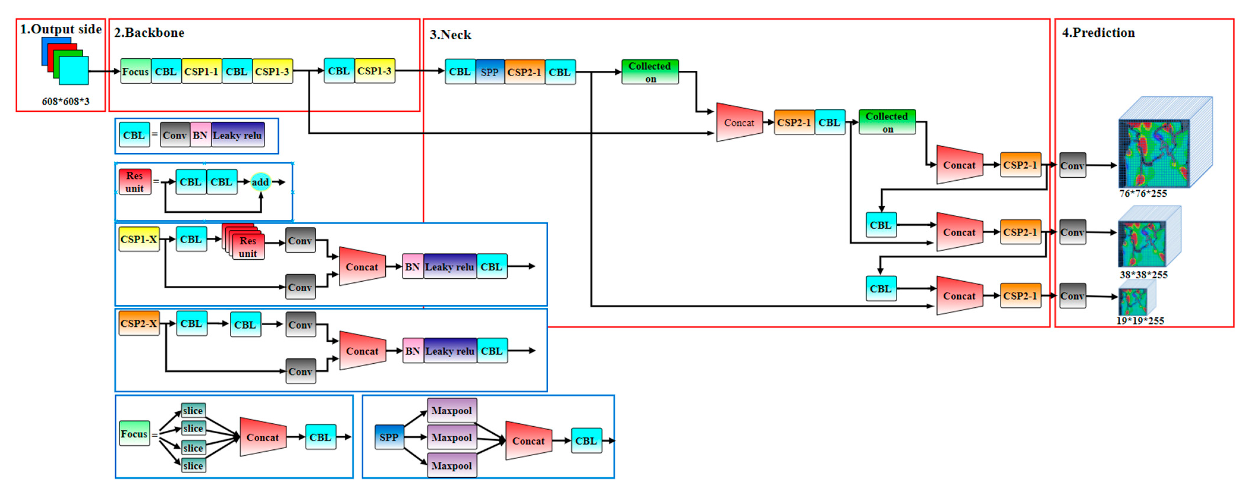
2. Principle and Development of YOLOv5
- (1)
- The input fracture network graph was divided into S × S grids. Each grid generated a prior frame for targets of different scales, responsible for tracking and recognizing the target when the centre of the target was located in a certain grid. The confidence degree c was used to represent the probability of target classification and the performance of target matching in the prior frame [32]:
- (2)
- The divided fracture images were normalized, and the normalized fracture dataset was sent to the underlying feature extraction network for feature extraction.
- (3)
- The prediction frame was divided into different sizes. For different detection targets, the position of the prediction frame, namely, the coordinate of the central point, was calculated.
- (4)
- According to the offset value of the predicted coordinates, the target center point position and the width and height of the prediction frame were calculated.
- (5)
- The target identification results were output.
3. Failure Test of the Fractured Rock Specimen
3.1. Preparation of Rock Specimens with Complex Fractures
3.1.1. 3D Printing of the Fracture Network Model
3.1.2. Preparation of Similar Rock Material Specimens for the Fracture Network
- (1)
- The specimen mould was selected with an internal size of 100 × 100 × 20 mm (length × width × height), and the 3D fracture solid model was placed in the mould. Cement mortar, with a material ratio of ordinary Portland cement:sand:water = 1:1:0.4, was poured into the mould, and full oscillation was achieved.
- (2)
- The mould was removed after 27 h, and the specimen was placed in a standard curing room for 28 days.
- (3)
- After curing, the specimen was immersed in clean water for 48 h, and the PVA material was dissolved, forming a fracture network.
- (4)
- The specimen was dried naturally at room temperature and polished smoothly with sandpaper. White paint and black paint were sprayed successively on one side of the specimen to form a speckled field. The white paint was the color base, and the black paint particles naturally fell on the white primer, which conveniently allowed the DIC equipment to collect and calculate the strain field.
3.2. Test Instrument
4. Test Results and Analysis
4.1. Mechanical Properties of the Specimens
- (1)
- All the pictures captured during the loading damage to the specimen were extracted from the camera. Based on the duration of the test piece damage phase, the feature pictures were taken as the observation objects.
- (2)
- The feature pictures were imported into the digital image correlation calculation software (Vic-2D), and the strain field cloud map and strain field data information obtained by digital image correlation calculation, where each picture had a set of strain field data information, all saved in Excel format.
- (3)
- The strain field information from the separate Excel tables was summarized into one table using a Python program, to obtain the strain field variation with time order.
- (1)
- In the initial compaction stage (0–a), similar to the real rock specimen, with significant initial nonlinear deformation characteristics, the original microdefects inside the specimen are gradually compacted. At this time, the precast fractures in the specimen did not propagate, and the strain field of the specimen was relatively uniform.
- (2)
- In the approximate linear stage (a–c), the stress–strain curve increased approximately linearly with increasing load. At point b, strain concentration occurred at the No. 17 fracture, but it had little effect on the overall strength of the specimen.
- (3)
- In the fracture initiation and propagation stage (c–f), when the stress increased to point c, strain concentration and fracture propagation occurred at the No. 2, 3, 11, 12, 14, and 17 fractures of the specimen. After c and before f, the stress–strain curve was accompanied by multiple stress drops and stress redistribution. In this process, although some new fractures were generated in the specimen, no surface-penetrating fracture appeared.
- (4)
- In the postpeak stage (f–h), when the stress reached the peak stress point f, the new fracture and the original fracture were connected in the specimen, and the bearing capacity of the specimen decreased rapidly, resulting in brittle failure. This indicates that the failure process of the fracture network specimens incorporated the germination and expansion of new fractures, and the bonding and coalescence of primary fractures.
4.2. Local Strain Response of Dynamic Fractures
- (1)
- In the initial compaction stage, the strain field of the specimen was relatively uniform, and only a small number of primary crack tips showed strain concentrations, which were not obvious and did not affect the overall basic strength of the specimen.
- (2)
- In the approximate linear stage, at point c, the ends of the No. 2, 3, 11, 12, 14, and 17 prefabricated fractures began to generate new fractures, and a dark red strain concentration area covering the fractures appeared in the strain field cloud map. At the same time, the elastic stage came to an end, and multiple fractures were initiated simultaneously.
- (3)
- In the fracture initiation and propagation stage, at point d, the No. 1, 2 and 3 prefabricated fractures on the left side of the specimen began to overlap with each other, and the left side was close to detaching. At the same time, the anti-wing fracture sprouting at the upper end of the No. 11 fracture was observed to overlap with that of the No. 13 fracture, and the wing fracture at the lower end of the No. 11 fracture overlapped with the anti-wing fractures at the upper ends of the No. 12 fractures. There was overlap between the reverse wing fractures generated at the upper end of No. 12 and the lower end of No. 14, and the wing fractures generated at the lower end of No. 17 and the upper end of No. 14 also overlapped. The positions of the above fractures in the strain field cloud map demonstrated significant changes. When the fracture propagation was significant, the strain data of the new fractures were lost, and the strain cloud map shows no colour. At the same time, the stress–strain curve was observed to show a small amplitude stress fluctuation.
- (4)
- In the postpeak stage, at point f, a wing fracture extending upwards germinated at the upper end of fracture No. 4, and an inclined anti-wing fracture at the lower end of fracture No. 6 overlapped with a wing fracture at the upper end of fracture No. 7. At point g, the fractures developed continuously, the new wing fractures at the top of fracture No. 4 developing to the edge of the specimen, inclined reverse wing fractures germinating at the top of fractures No. 6 and No. 7. Inclined secondary fractures germinated in the middle of fracture No. 13, and the tensile wing fractures at the bottom of fracture No. 14 propagated along the axis, resulting in a stress drop of 1.14 MPa in the stress–strain curve. At point h, the wing fracture generated at the upper end of fracture No. 9 overlapped with the reverse wing fracture generated at the lower end of fracture No. 12, and the prefabricated fractures 4, 5, 6, 7, 8, 9, 11, 12, 13, 14, and 17 overlapped with each other to form a complex fracture network, resulting in a stress drop and eventually forming a macroscopic penetrating fracture leading to failure of the specimen.
5. Intelligent Detection of Dynamic Fractures
5.1. Experimental Treatment and Results
5.1.1. Software and Hardware Conditions
5.1.2. Dataset
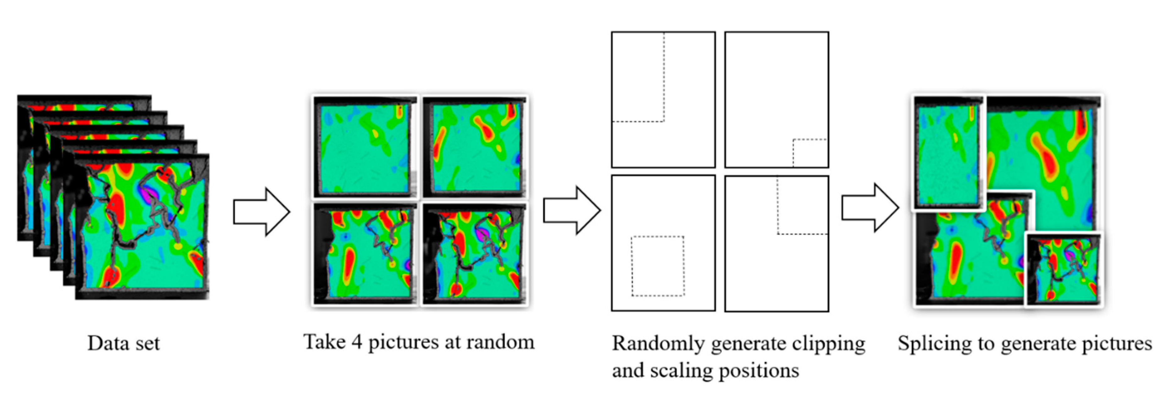
- (1)
- Dataset preprocessing
- (2)
- Fracture classification
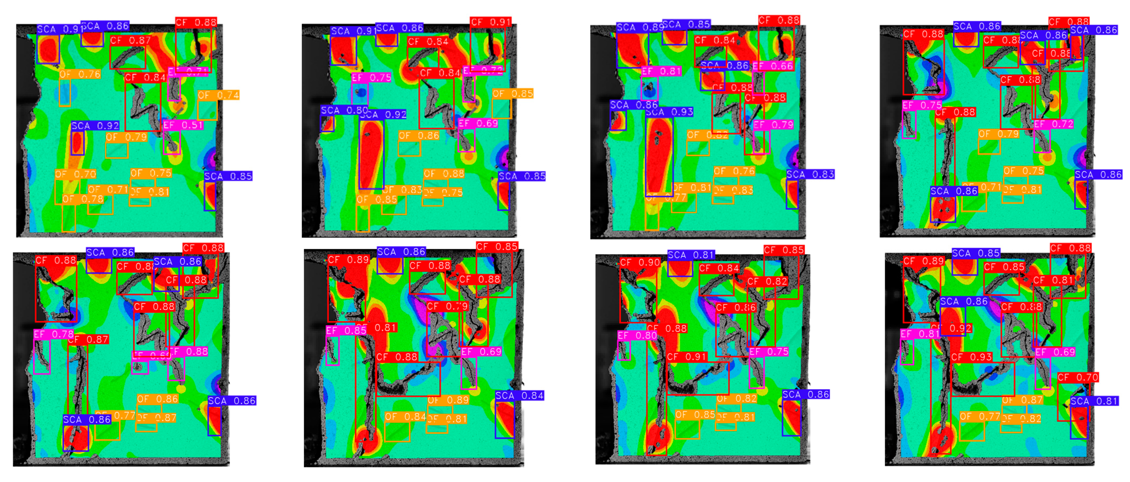
5.1.3. Test Results
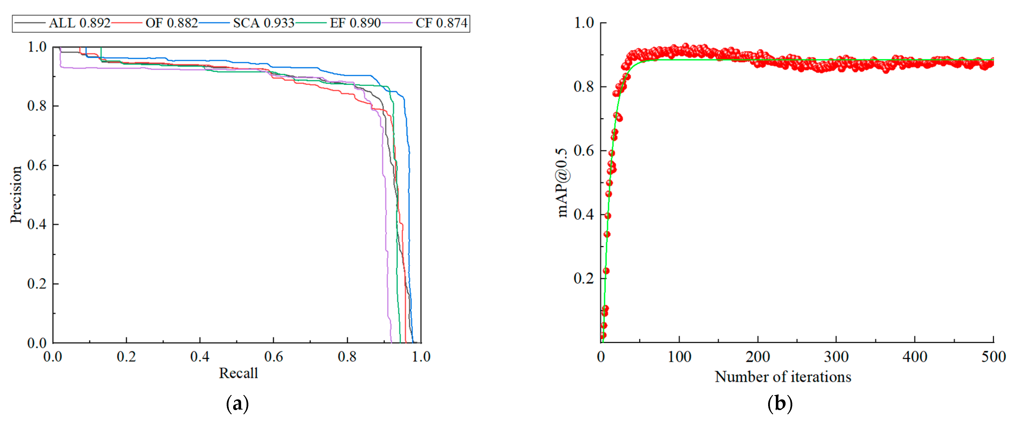
5.2. Algorithm Evaluation
5.2.1. Measurement Index of Model Recognition Accuracy
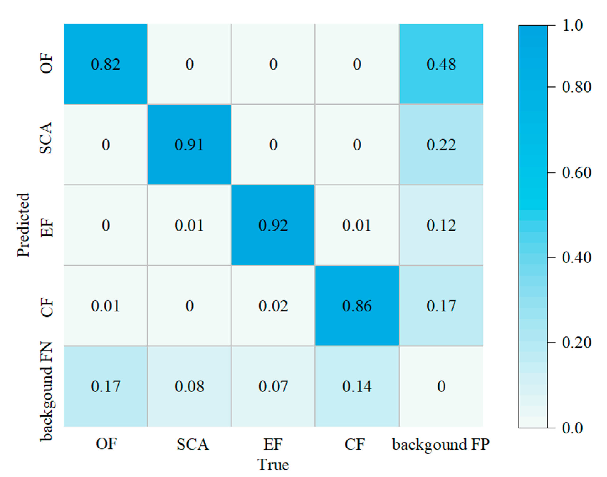
5.2.2. Evaluation Results
6. Conclusions
- (1)
- The failure process of specimens with complex fractures is often accompanied by the propagation and coalescence of multiple dynamic fractures. DIC monitoring showed that before the initiation of each primary fracture, the strain concentration area always appeared first, which indicated the initiation of new fractures.
- (2)
- There was an important relationship between the overall strength of the specimen and the propagation of a single fracture. At the end of the elastic deformation stage, the stress was close to its peak, at approximately 97% of peak stress. In the fracture propagation stage, there were many stress fluctuations, which had an important relationship with the cross fractures. After reaching peak stress, the specimen was rapidly destroyed. The overall strength of the specimen can be evaluated semiquantitatively by the statistics of the expansion of each fracture.
- (3)
- Based on the strength law and strain field cloud map of specimens, the dynamic evolution of primary fractures can be divided into four types: primary fractures, stress concentration area, new fractures, and cross fractures, among which the cross fractures had the greatest impact on the overall strength of the specimen.
- (4)
- Based on YOLOv5, an intelligent detection algorithm for identifying dynamic fractures in rock specimens with complex fractures was established. The detection results show that the value of mAP@0.5 was above 80%, reaching 91%. This model can be used for intelligent and accurate identification of dynamic fractures, and the state of each fracture can be determined intelligently based on the type of fracture.
- (5)
- The established intelligent detection model of dynamic fractures demonstrated fast detection speed and high accuracy. The F1 corresponding to the four fracture types was 85%, 91%, 89%, and 87%, and the overall identification accuracy reached 86%.
- (6)
- In underground coal mine engineering, crack expansion and penetration may occur until rupture channels appear, for various reasons such as cyclic mining and gas seepage surges, with potential for disaster. This paper proposes a combination of the YOLOv5 deep learning network model and DIC technology, for the intelligent detection and identification of crack extensions in complex rock specimens. The experimental evaluation has shown that the method is fast, accurate, and effective in the identification, localization, and classification of cracks in complex fractured rock masses. Therefore, it is proposed that intelligent monitoring of rock damage can be realized to provide improved damage warning and directions for engineering safety protection.
Author Contributions
Funding
Institutional Review Board Statement
Informed Consent Statement
Data Availability Statement
Acknowledgments
Conflicts of Interest
References
- Chen, W.; Li, S.; Zhu, W.; Qiu, X. Experimental and numerical research on crack propagation rock under compression. Chin. J. Rock Mech. Eng. 2003, 22, 18–23. (In Chinese) [Google Scholar]
- Liu, X.; Zhu, W.; Zhang, P.; Li, L. Failure in rock with intersecting rough joints under uniaxial compression. Int. J. Rock Mech. Min. Sci. 2021, 146, 104832. [Google Scholar] [CrossRef]
- Sivakumar, G.; Maji, V.B. Crack Growth in Rocks with Preexisting Narrow Flaws under Uniaxial Compression. Int. J. Geomech. 2021, 21, 04021032. [Google Scholar] [CrossRef]
- Lin, H.; Sheng, B. Failure Characteristics of Complicated Random Jointed Rock Mass Under Compressive-Shear Loading. Geotech. Geol. Eng. 2021, 39, 3417–3435. [Google Scholar] [CrossRef]
- Wang, H.; Zhang, B.; Yuan, L.; Wang, S.; Yu, G.; Liu, Z. Analysis of precursor information for coal and gas outbursts induced by roadway tunneling: A simulation test study for the whole process. Tunn. Undergr. Space Technol. 2022, 122, 104349. [Google Scholar] [CrossRef]
- Miao, S.; Pan, P.Z.; Wu, Z.; Li, S.; Zhao, S. Fracture analysis of sandstone with a single filled flaw under uniaxial compression. Eng. Fract. Mech. 2018, 204, 319–343. [Google Scholar] [CrossRef]
- Jin, Z.; Johnson, S.; Fan, Z. Subcritical propagation and coalescence of oil-filled cracks: Getting the oil out of low-permeability source rocks. Geophys. Res. Lett. 2010, 37. [Google Scholar] [CrossRef] [Green Version]
- Fan, Z.; Jin, Z.; Johnson, S. Oil-Gas Transformation Induced Subcritical Crack Propagation and Coalescence in Petroleum Source Rocks. Int. J. Fract. 2014, 185, 187–194. [Google Scholar] [CrossRef]
- Wang, X.; Wang, E.; Liu, X.; Zhou, X. Failure mechanism of fractured rock and associated acoustic behaviors under different loading rates. Eng. Fract. Mech. 2021, 247, 107674. [Google Scholar] [CrossRef]
- Ma, G.; Li, M.; Wang, H.; Chen, Y. Equivalent discrete fracture network method for numerical estimation of deformability in complexly fractured rock masses. Eng. Geol. 2020, 277, 105784. [Google Scholar] [CrossRef]
- Luo, K.; Zhao, G.; Zeng, J.; Zhang, X.; Pu, C. Fracture experiments and numerical simulation of cracked body in rock-like materials affected by loading rate. Chin. J. Rock Mech. Eng. 2018, 37, 1833–1842. (In Chinese) [Google Scholar]
- Suzuki, A.; Watanabe, N.; Li, K.; Horne, R.N. Fracture network created by 3-D printer and its validation using CT images. Water Resour. Res. 2017, 53, 6330–6339. [Google Scholar] [CrossRef]
- Munoz, H.; Taheri, A. Specimen aspect ratio and progressive field strain development of sandstone under uniaxial compression by three-dimensional digital image correlation. J. Rock Mech. Geotech. Eng. 2017, 9, 599–610. [Google Scholar] [CrossRef]
- Cao, R.; Lin, H.; Cao, P. Strength and failure characteristics of brittle jointed rock-like specimens under uniaxial compression: Digital speckle technology and a particle mechanics approach. Int. J. Min. Sci. Technol. 2018, 28, 669–677. [Google Scholar] [CrossRef]
- Deepanshu, S.; Ahmadreza, H.; Gabriel, W. Damage monitoring in rock specimens with pre-existing flaws by non-linear ultrasonic waves and digital image correlation. Int. J. Rock Mech. Min. Sci. 2021, 142, 1–18. [Google Scholar]
- Wang, B.; Jin, A.; Sun, H.; Wang, S. Study on the rupture mechanism of 3D printed rough cross-sectional specimens containing different angles based on DIC. Rock Soil Mech. 2021, 42, 439–450. (In Chinese) [Google Scholar]
- Zhang, K.; Qi, F.F.; Chen, Y.L. Deformation and fracturing characteristics of fracture network model and influence of filling based on 3D printing and DIC technologies. Rock Soil Mech. 2020, 41, 2555–2563. (In Chinese) [Google Scholar]
- Zhang, K.; Zhang, K. Gray and texture features of strain field for fractured sandstone during failure process. J. China Coal Soc. 2021, 46, 1253–1262. (In Chinese) [Google Scholar]
- Kou, X.; Liu, S.; Cheng, K.; Qian, Y. Development of a YOLO-V3-based model for detecting defects on steel strip surface. Measurement 2021, 182, 109454. [Google Scholar] [CrossRef]
- Zhang, J.; Yang, X.; Li, W.; Zhang, S.; Jia, Y. Automatic detection of moisture damages in asphalt pavements from GPR data with deep CNN and IRS method. Autom. Constr. 2020, 113, 103119. [Google Scholar] [CrossRef]
- Hamed, M.; Yaw, A.G.; William, G.B. Deep machine learning approach to develop a new asphalt pavement condition index. Constr. Build. Mater. 2020, 247, 118513. [Google Scholar]
- Ju, H.; Li, W.; Tighe, S.; Zhai, J.; Xu, Z.; Chen, Y. Detection of sealed and unsealed cracks with complex backgrounds using deep convolutional neural network. Autom. Constr. 2019, 107, 102946. [Google Scholar]
- Cui, X.; Wang, Q.; Dai, J.; Zhang, R.; Li, S. Intelligent recognition of erosion damage to concrete based on improved YOLO-v3. Mater. Lett. 2021, 302, 130363. [Google Scholar] [CrossRef]
- Jiang, Y.; Pang, D.; Li, C. A deep learning approach for fast detection and classification of concrete damage. Autom. Constr. 2021, 128, 103785. [Google Scholar] [CrossRef]
- Wei, F.; Yao, G.; Yang, Y.; Sun, Y. Instance-level recognition and quantification for concrete surface bughole based on deep learning. Autom. Constr. 2019, 107, 102920. [Google Scholar] [CrossRef]
- Song Ee, P.; Seung-Hyun, E.; Haemin, J. Concrete crack detection and quantification using deep learning and structured light. Constr. Build. Mater. 2020, 252, 119096. [Google Scholar]
- Yan, P.; Sun, Q.; Yin, N.; Hua, L.; Shang, S.; Zhang, C. Detection of coal and gangue based on improved YOLOv5.1 which embedded scSE module. Measurement 2022, 188, 110530. [Google Scholar] [CrossRef]
- Tan, Y.; Cai, R.; Li, J.; Chen, P.; Wang, M. Automatic detection of sewer defects based on improved you only look once algorithm. Autom. Constr. 2021, 131, 103912. [Google Scholar] [CrossRef]
- Haneul, C.; Chai, Y.U.; Kyungmo, K.; Hyungkeun, K.; Taeyeon, K. Application of vision-based occupancy counting method using deep learning and performance analysis. Energy Build. 2021, 252, 111389. [Google Scholar]
- Wu, L.; Zhang, L.; Shi, J.; Zhang, Y.; Wan, J. Damage detection of grotto murals based on lightweight neural network. Comput. Electr. Eng. 2022, 102, 108237. [Google Scholar] [CrossRef]
- Shihavuddin, A.S.M.; Rashid, M.R.A.; Maruf, M.H.; Hasan, M.A.; ul Haq, M.A.; Ashique, R.H.; Al Mansur, A. Image based surface damage detection of renewable energy installations using a unified deep learning approach. Energy Rep. 2021, 7, 4566–4576. [Google Scholar] [CrossRef]
- Li, S.; Gu, X.; Xu, X.; Xu, D.; Zhang, T.; Liu, Z.; Dong, Q. Detection of concealed cracks from ground penetrating radar images based on deep learning algorithm. Constr. Build. Mater. 2021, 273, 121949. [Google Scholar] [CrossRef]
- Liu, Q.S.; He, F.; Deng, P.H.; Tian, Y.C. Application of 3D printing technology in physical modelling in rock mechanics. Rock Soil Mech. 2019, 40, 3397–3404. (In Chinese) [Google Scholar]
- Deng, S.; Wang, X.; Yu, J.; Zhang, Y.; Liu, Z.; Zhu, Y. Simulation of Grouting Process in Rock Masses Under a Dam Foundation Characterized by a 3D Fracture Network. Rock Mech. Rock Eng. 2018, 51, 1801–1822. [Google Scholar] [CrossRef]
- Li, R.; Hu, X.; Chen, F.; Wang, X.; Xiong, H.; Wu, H. A systematic framework for DEM study of realistic gravel-sand mixture from particle recognition to macro- and micro-mechanical analysis. Transp. Geotech. 2022, 34, 100693. [Google Scholar] [CrossRef]
- Song, K.; Jung, J.Y.; Lee, S.H.; Park, S. A comparative study of deep learning-based network model and conventional method to assess beach debris standing-stock. Mar. Pollut. Bull. 2021, 168, 112466. [Google Scholar] [CrossRef]
- Zhang, F.; Ren, F.; Li, J.; Zhang, X. Automatic stomata recognition and measurement based on improved YOLO deep learning model and entropy rate superpixel algorithm. Ecol. Inform. 2022, 68, 101521. [Google Scholar] [CrossRef]


| Material Type | Density ρ/g·cm−3 | Uniaxial Compressive Strength σc/MPa | Elastic Modulus E/GPa | Poisson’s Ratio μ | Tensile Strength σt/MPa |
|---|---|---|---|---|---|
| Mortar | 2.04 | 80.26 | 11.2 | 0.18 | 5.42 |
| Points | Fissure Development | Strain Fields | Points | Fissure Development | Strain Fields |
|---|---|---|---|---|---|
| a |  | 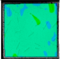 | b |  | 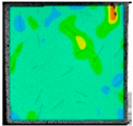 |
| c |  |  | d |  | 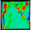 |
| e |  | 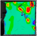 | f |  | 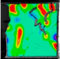 |
| g |  |  | h |  | 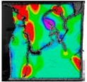 |
| No. | 1 | 2 | 3 | 4 | 5 | 6 | 7 | 8 | 9 | 10 | 11 | 12 | 13 | 14 | 15 | 16 | 17 | 18 | 19 | 20 |
|---|---|---|---|---|---|---|---|---|---|---|---|---|---|---|---|---|---|---|---|---|
| a | ○ | ○ | ○ | ○ | ○ | ○ | ○ | ○ | ○ | ○ | ○ | ○ | ○ | ○ | ○ | ○ | ○ | ○ | ○ | ○ |
| b | ○ | ○ | ○ | ○ | ○ | ○ | ○ | ○ | ○ | ○ | ○ | ○ | ○ | ○ | ○ | ○ | ○ | ○ | ○ | ○ |
| c | ○ | □ | □ | ○ | ○ | ○ | ○ | ○ | ○ | ○ | □ | □ | ○ | □ | ○ | ○ | □ | ○ | ○ | ○ |
| d | □ | □ | △ | ○ | ○ | ○ | ○ | ○ | ○ | ○ | □ | □ | □ | □ | ○ | ○ | □ | ○ | ○ | ○ |
| e | △ | △ | △ | ○ | ○ | ○ | ○ | ○ | ○ | ○ | □ | □ | □ | □ | ○ | ○ | □ | ○ | ○ | ○ |
| f | △ | △ | △ | □ | ○ | □ | □ | ○ | ○ | ○ | □ | □ | □ | □ | ○ | ○ | □ | ○ | ○ | ○ |
| g | △ | △ | △ | □ | □ | □ | □ | ○ | ○ | ○ | □ | □ | □ | □ | ○ | ○ | □ | ○ | ○ | ○ |
| h | △ | △ | △ | □ | □ | □ | □ | □ | □ | ○ | □ | □ | □ | □ | ○ | ○ | □ | ○ | ○ | □ |
| Type | All | OF | SCA | EF | CF |
|---|---|---|---|---|---|
| F1 | 0.88 | 0.85 | 0.91 | 0.89 | 0.87 |
Publisher’s Note: MDPI stays neutral with regard to jurisdictional claims in published maps and institutional affiliations. |
© 2022 by the authors. Licensee MDPI, Basel, Switzerland. This article is an open access article distributed under the terms and conditions of the Creative Commons Attribution (CC BY) license (https://creativecommons.org/licenses/by/4.0/).
Share and Cite
Zhang, Q.; Zhang, B.; Chen, C.; Li, L.; Wang, X.; Jiang, B.; Zheng, T. A Test Method for Finding Early Dynamic Fracture of Rock: Using DIC and YOLOv5. Sensors 2022, 22, 6320. https://doi.org/10.3390/s22176320
Zhang Q, Zhang B, Chen C, Li L, Wang X, Jiang B, Zheng T. A Test Method for Finding Early Dynamic Fracture of Rock: Using DIC and YOLOv5. Sensors. 2022; 22(17):6320. https://doi.org/10.3390/s22176320
Chicago/Turabian StyleZhang, Qinghe, Bing Zhang, Chen Chen, Ling Li, Xiaorui Wang, Bowen Jiang, and Tianle Zheng. 2022. "A Test Method for Finding Early Dynamic Fracture of Rock: Using DIC and YOLOv5" Sensors 22, no. 17: 6320. https://doi.org/10.3390/s22176320
APA StyleZhang, Q., Zhang, B., Chen, C., Li, L., Wang, X., Jiang, B., & Zheng, T. (2022). A Test Method for Finding Early Dynamic Fracture of Rock: Using DIC and YOLOv5. Sensors, 22(17), 6320. https://doi.org/10.3390/s22176320