
Towards a Recommender System for In-Vehicle Antenna Placement in Harsh Propagation Environments


Abstract
:1. Introduction
1.1. State of the Art
1.2. Research Contribution
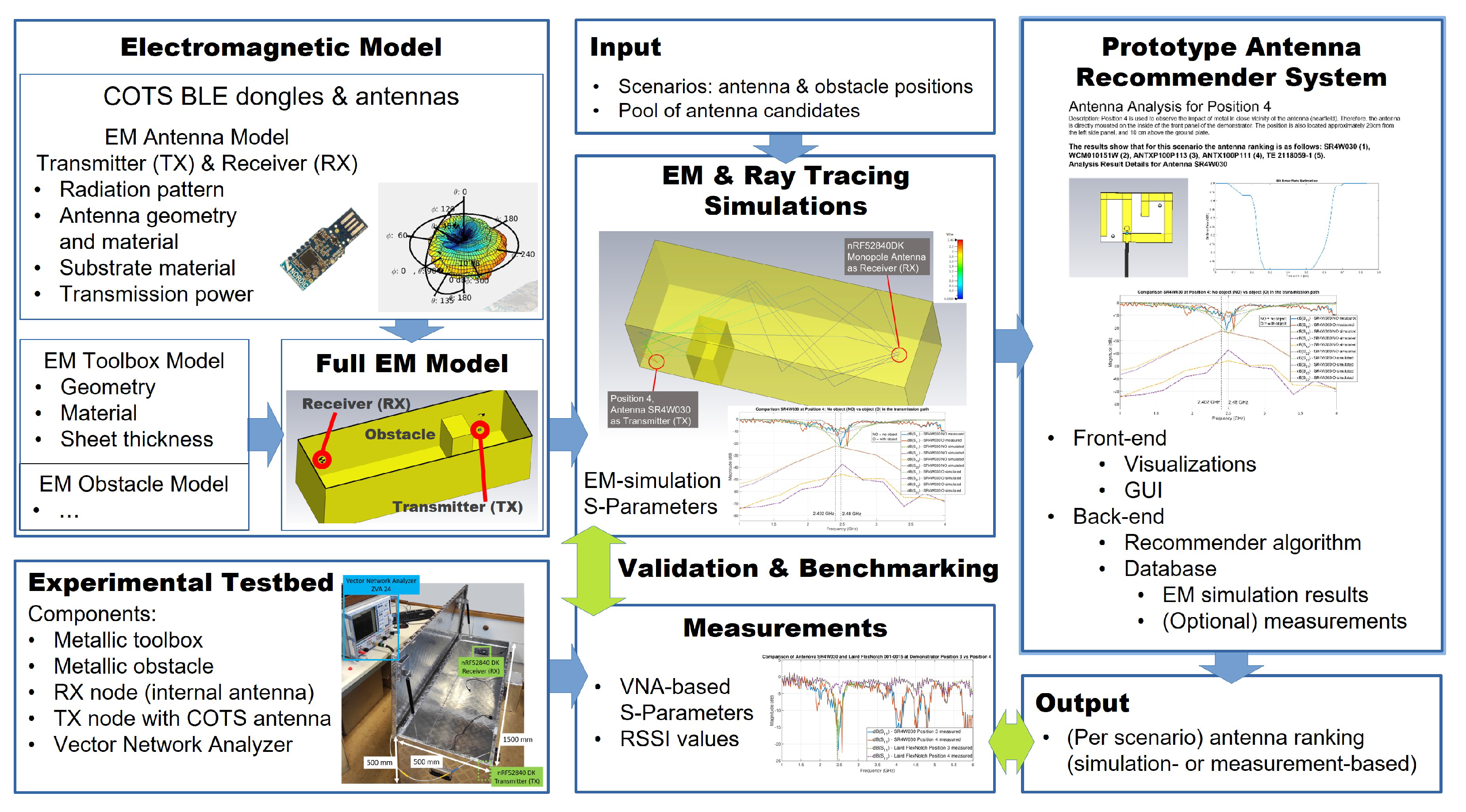
2. Concept Overview
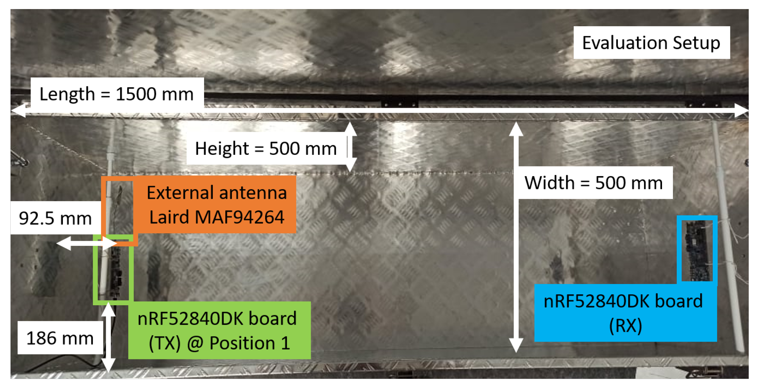
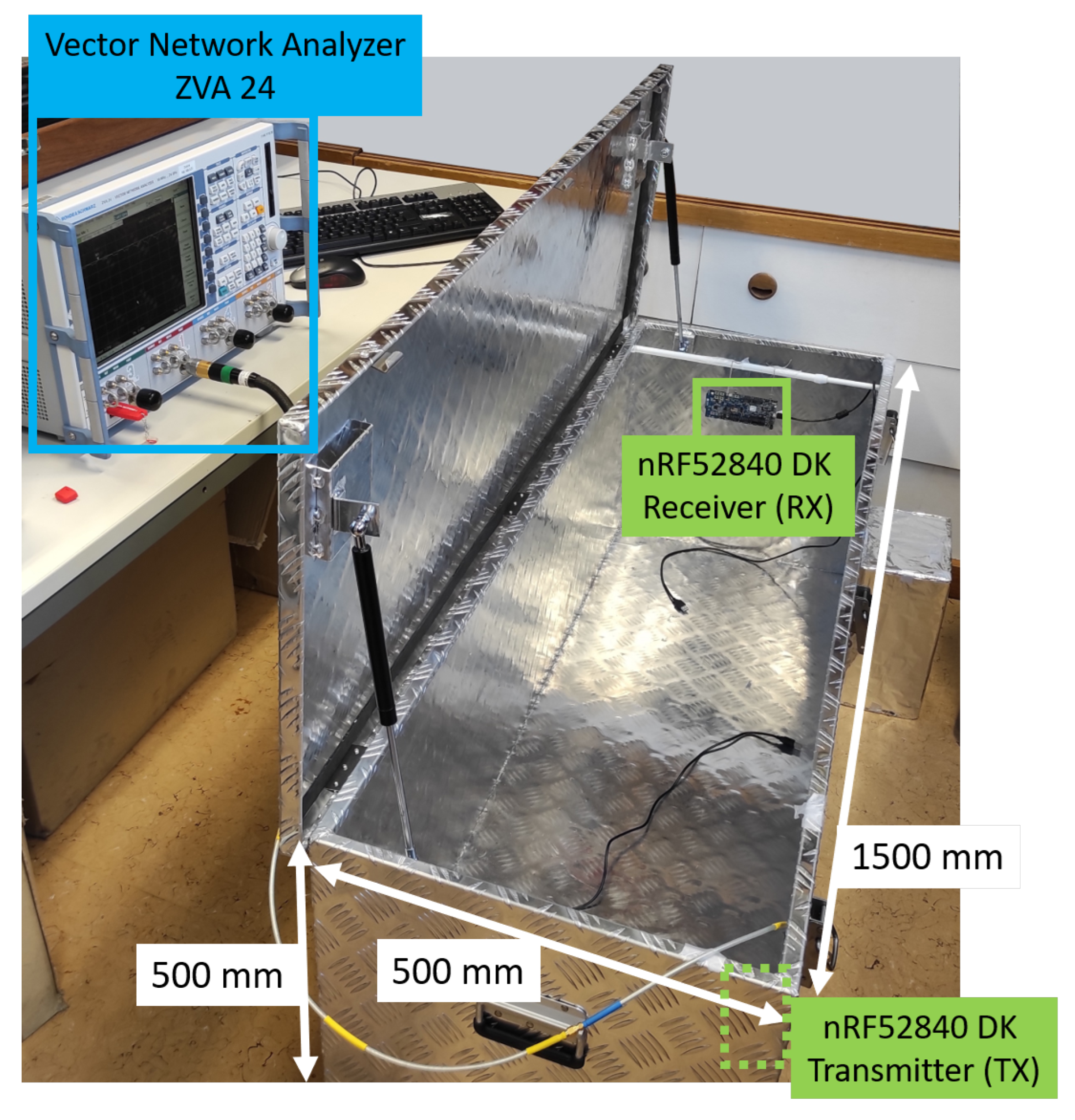
3. Experimental Testbed—Physical Mock-Up of an Engine Compartment
4. Electromagnetic Simulations of the Experimental Testbed
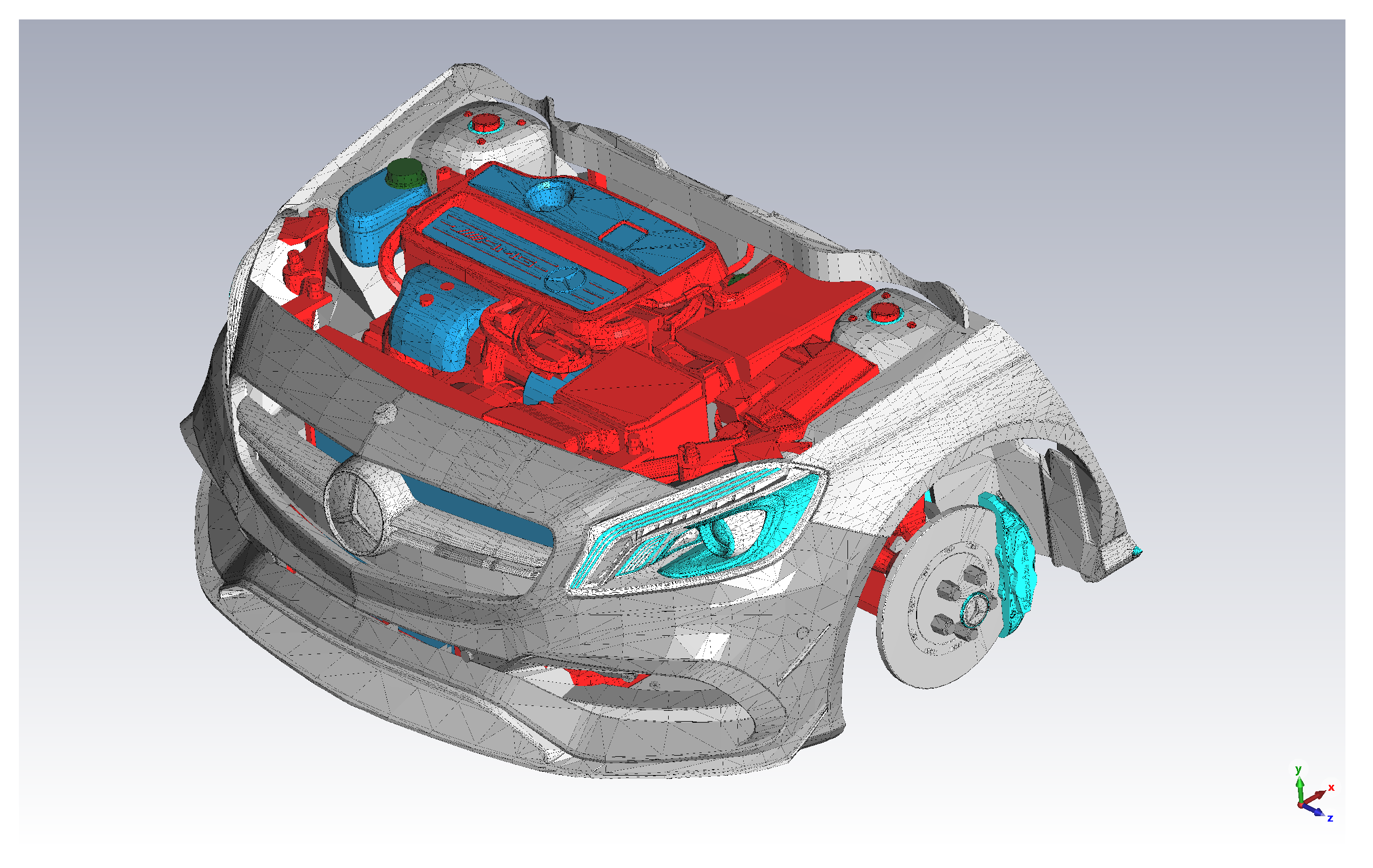
4.1. Full Electromagnetic Model
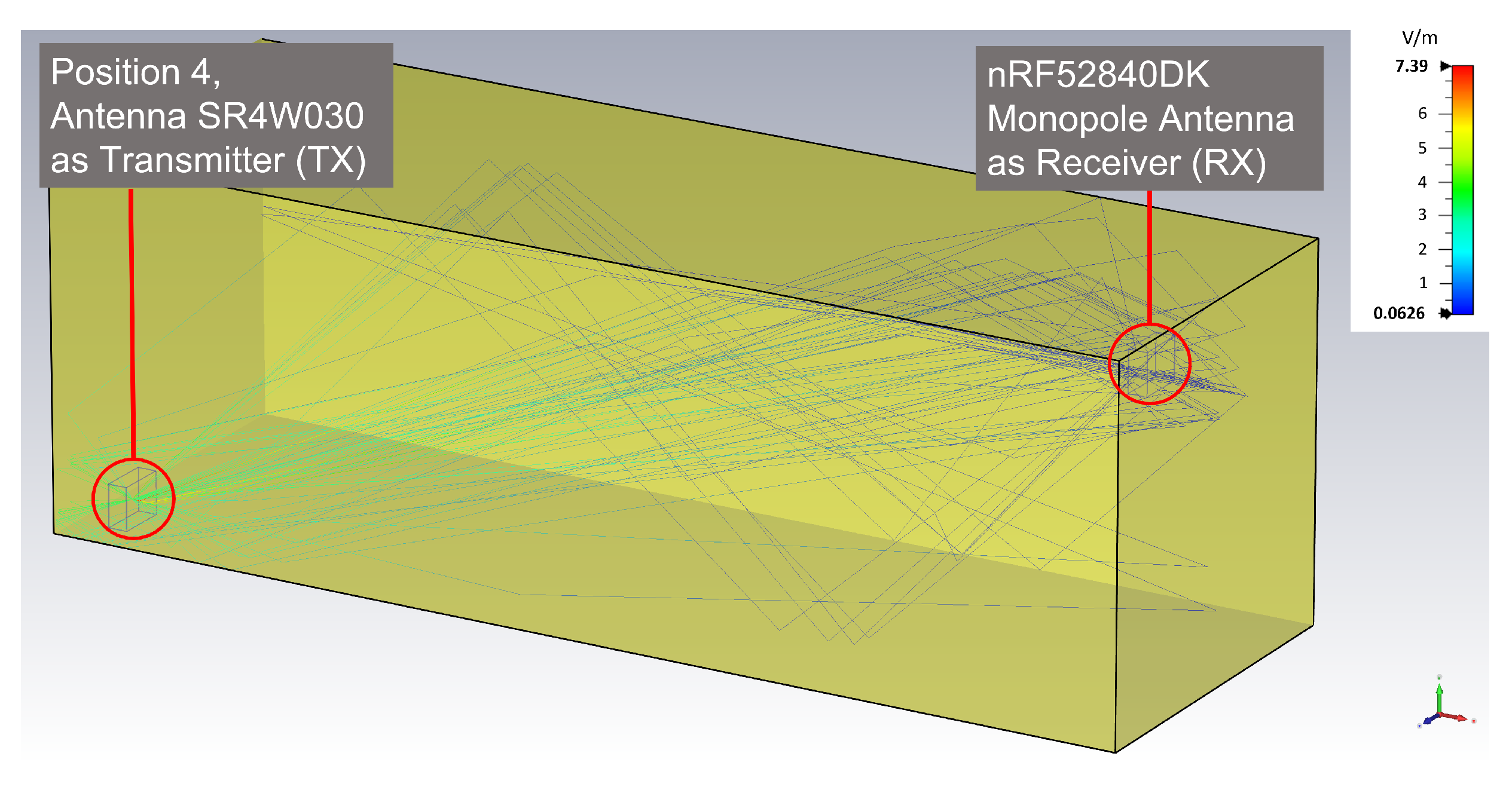
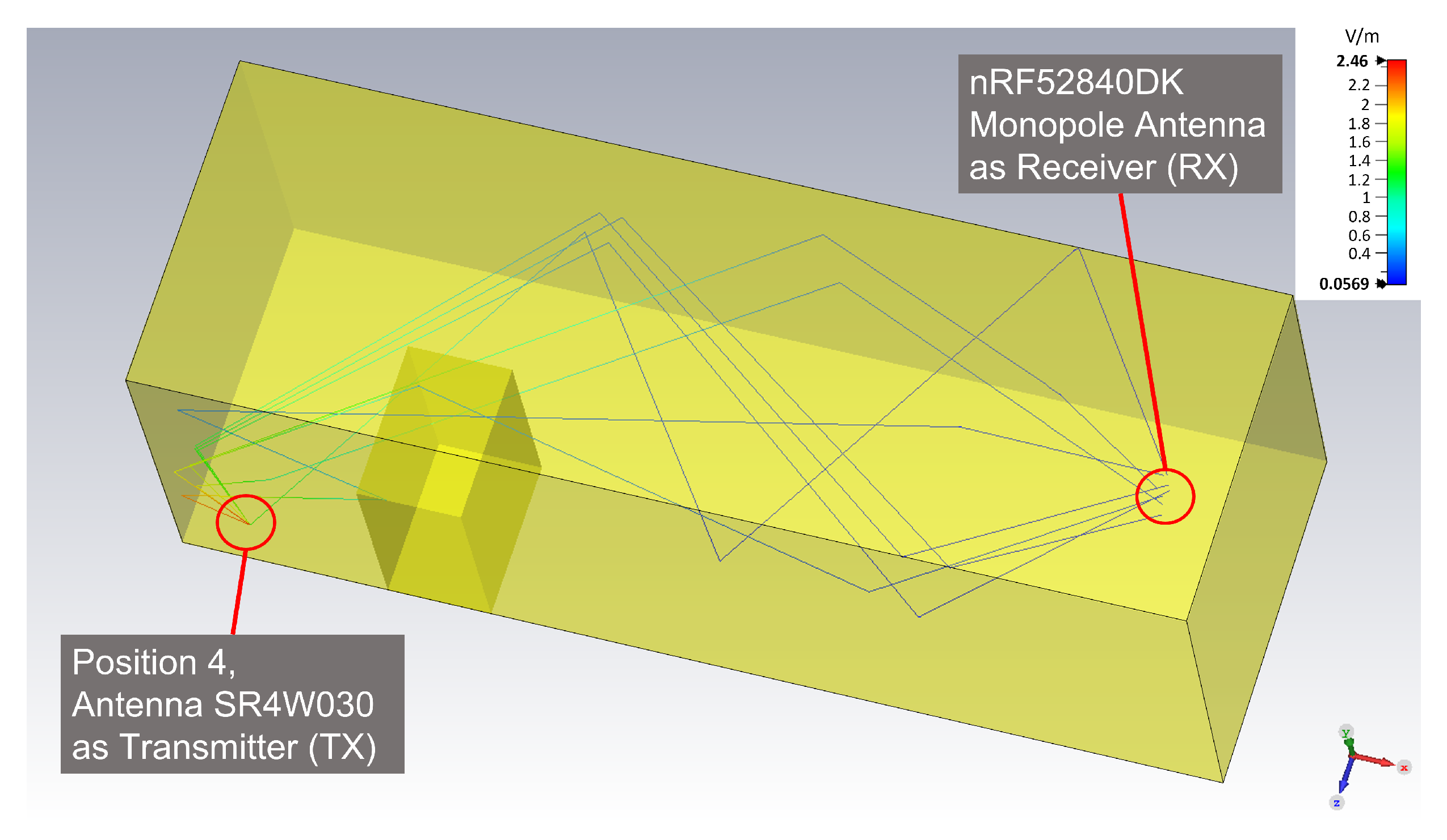
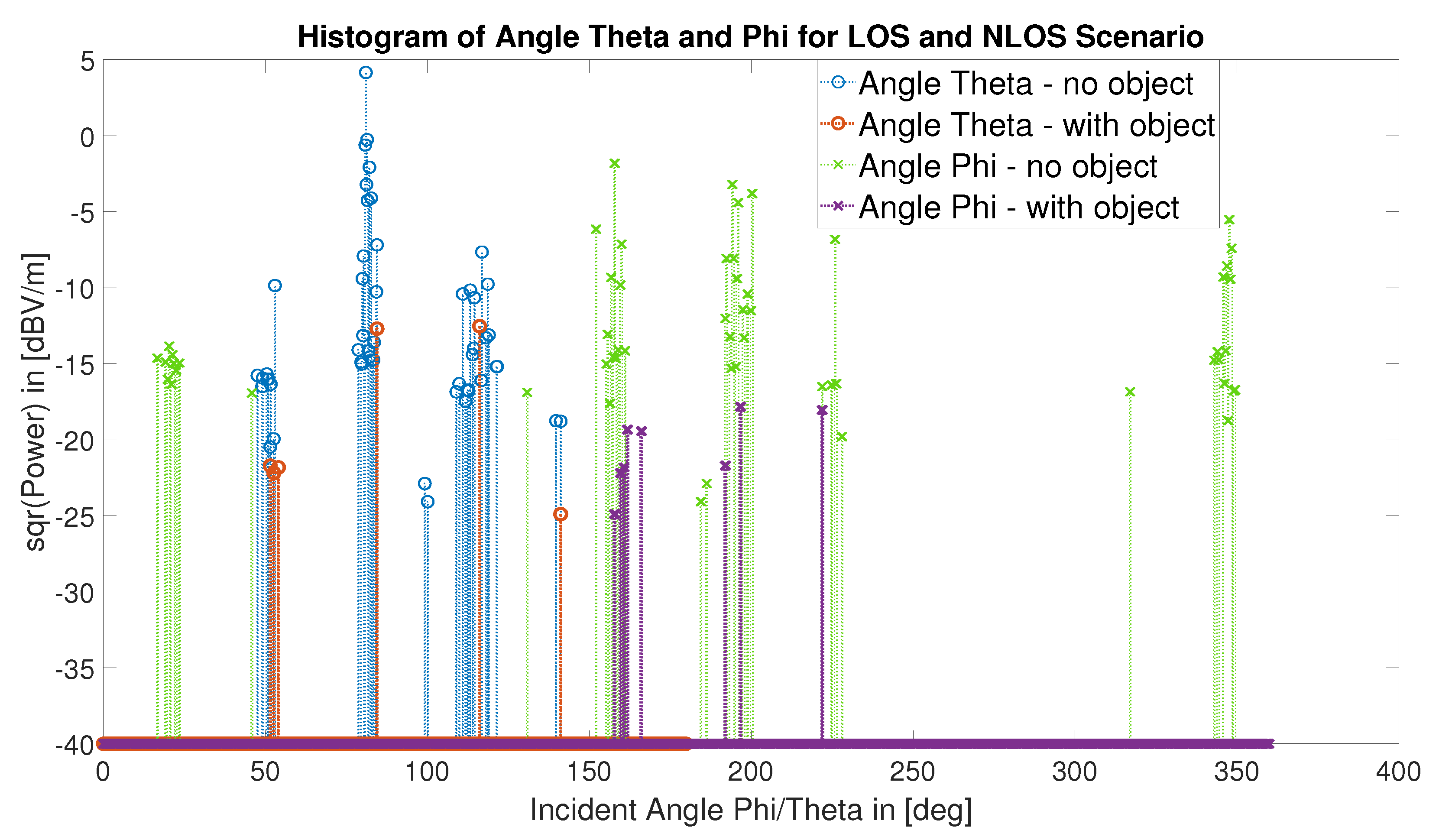
4.2. EM Ray-Tracing Simulation
5. Experimental Antenna Evaluations
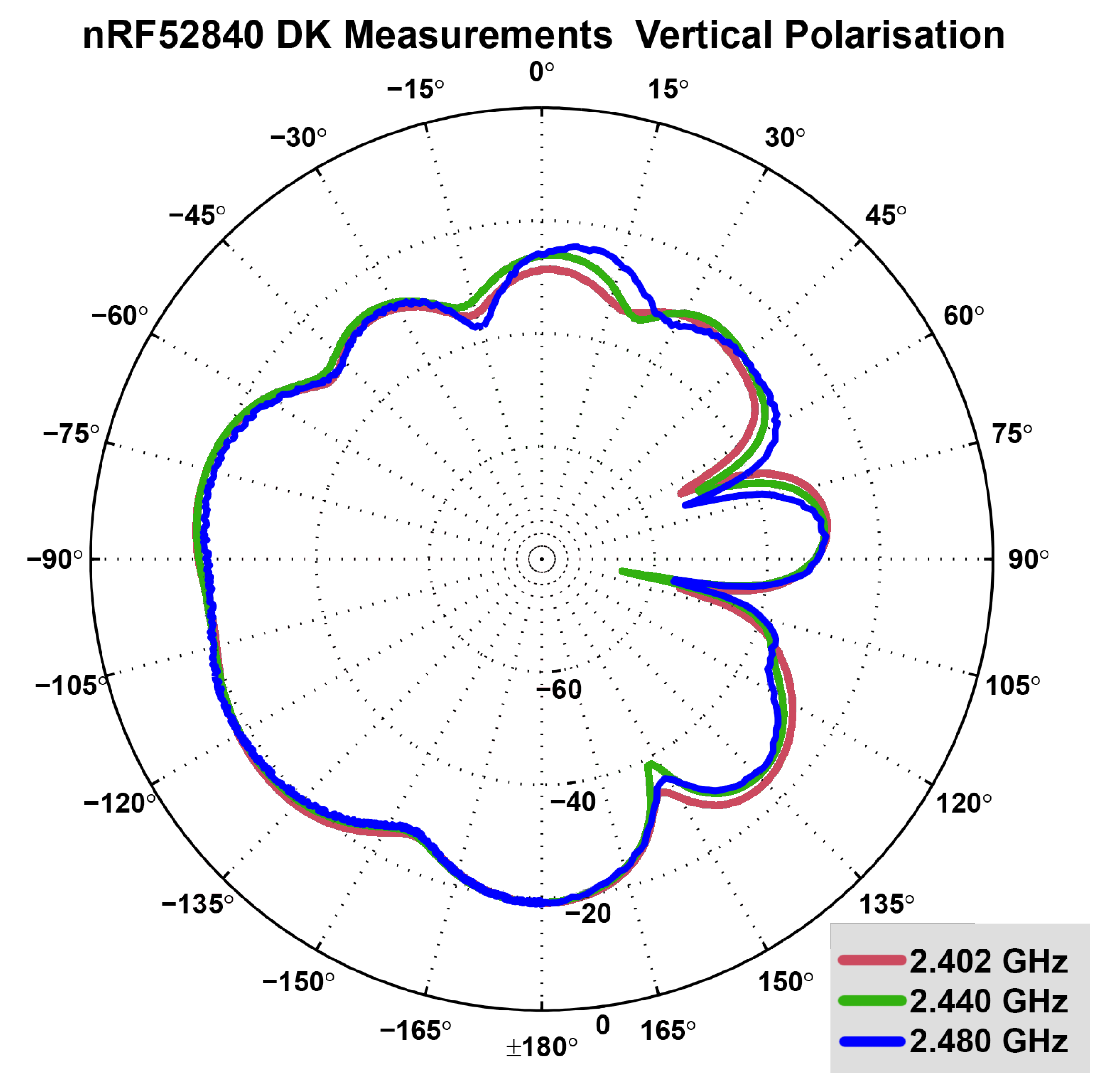
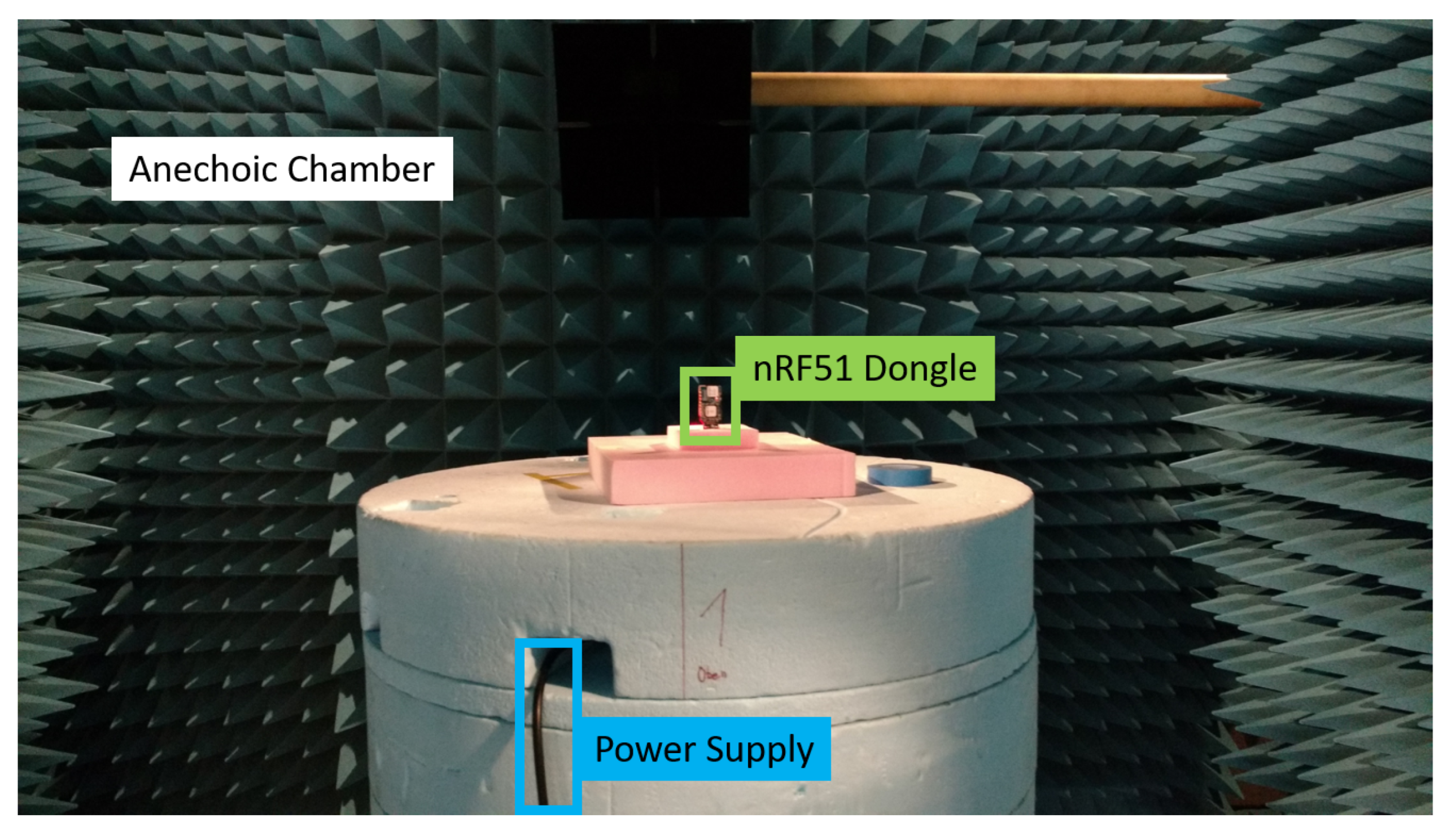
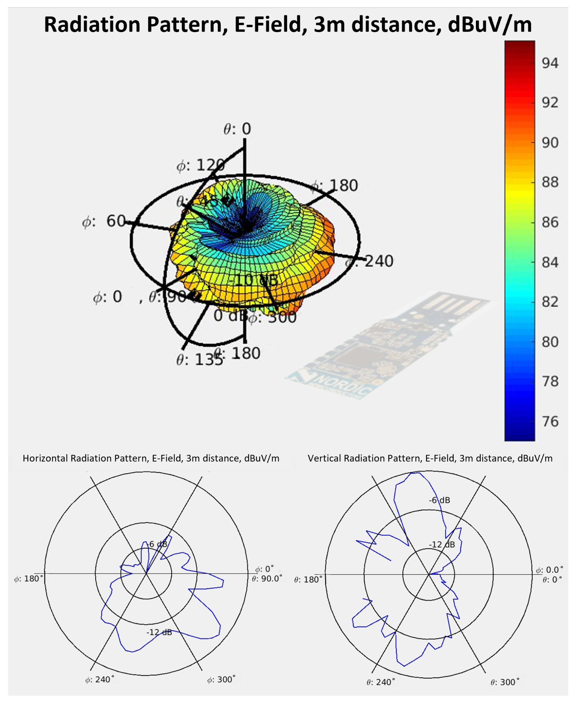
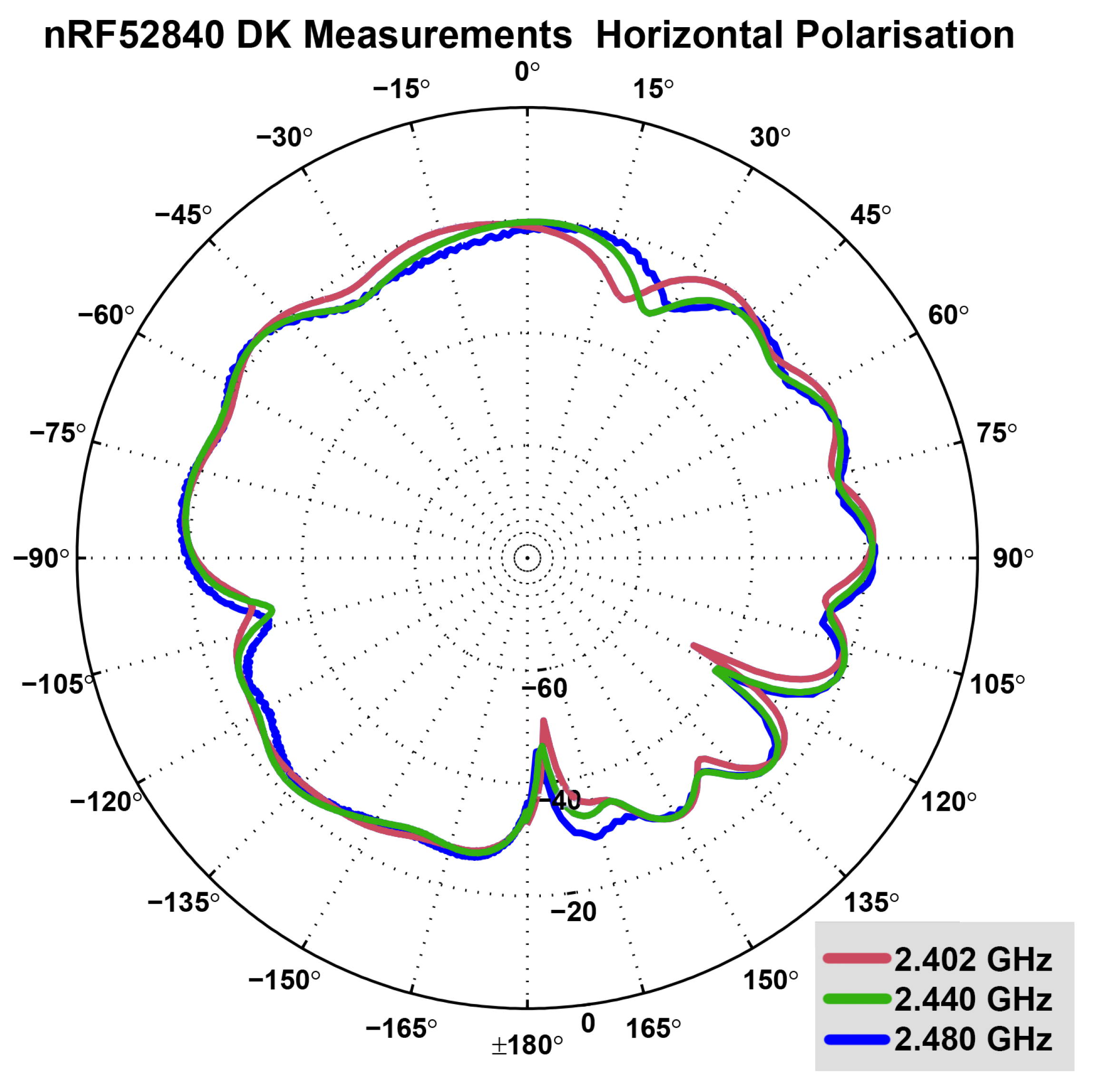
5.1. Antenna Radiation Patterns
5.2. Measurement of Wireless Communication Channel
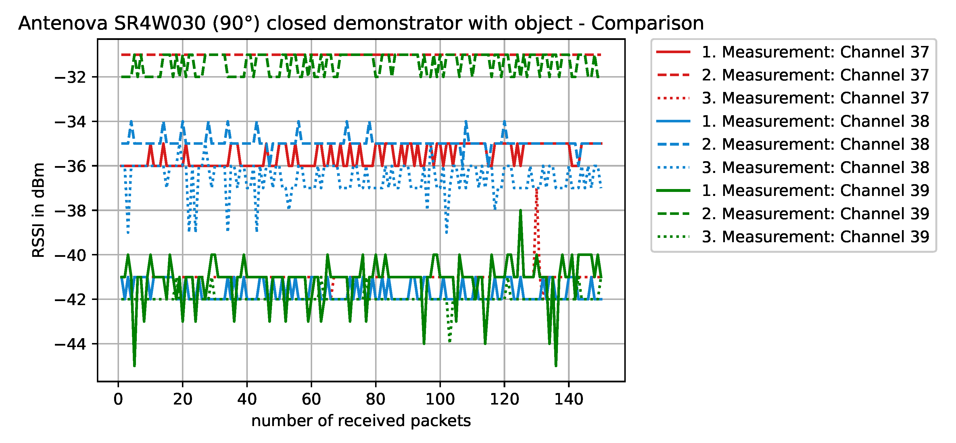
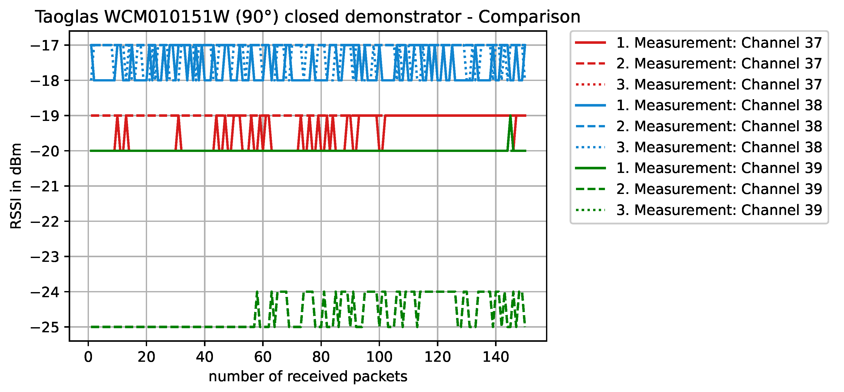
5.2.1. Received Signal Strength Indicator
5.2.2. Vector Network Analyzer Measurements
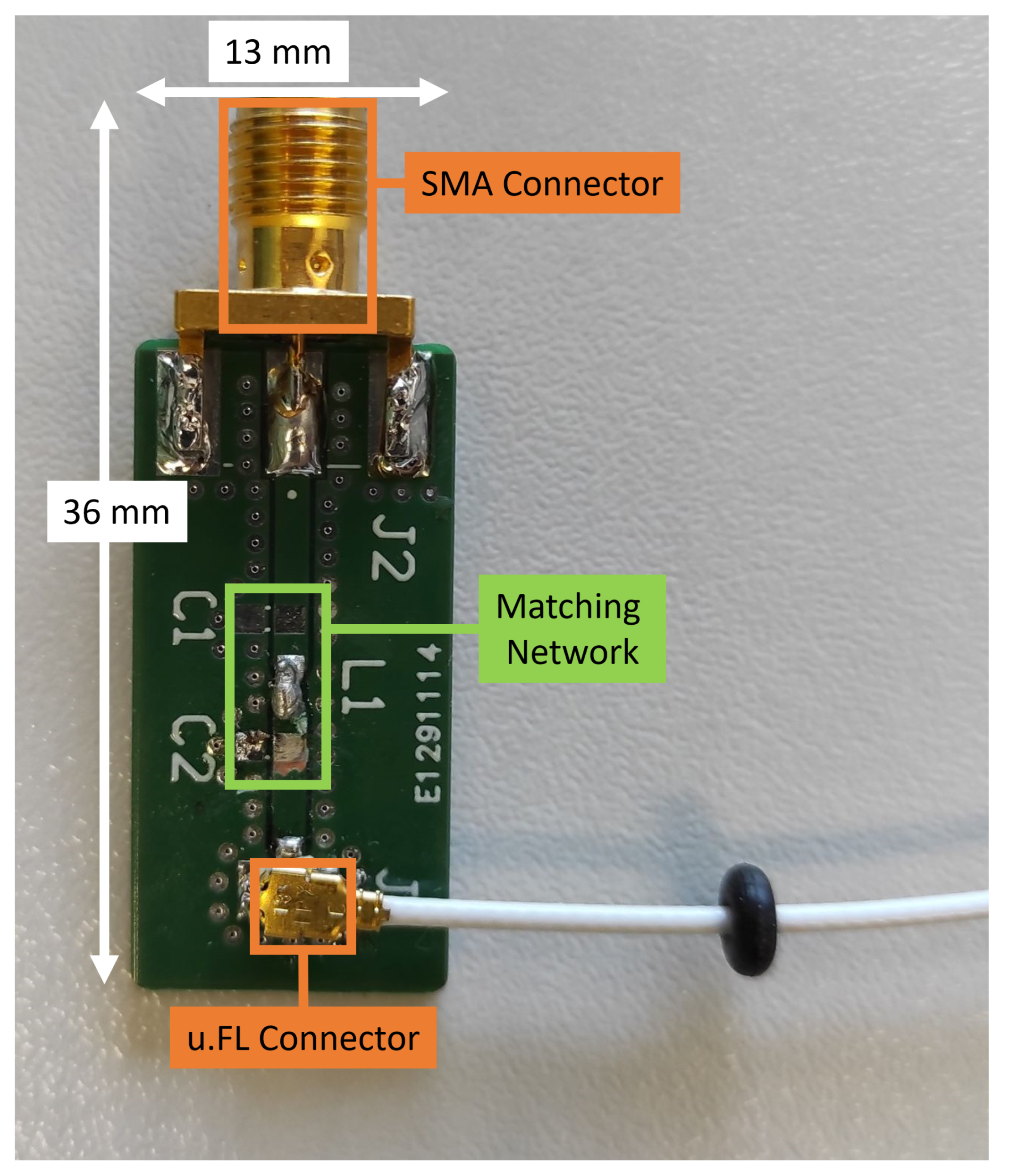
5.3. Additional Requirements for Measurements
6. Experimental Results
6.1. Experimental Setup
6.2. Preliminary Experimental Analysis
6.3. RSSI versus VNA Measurements
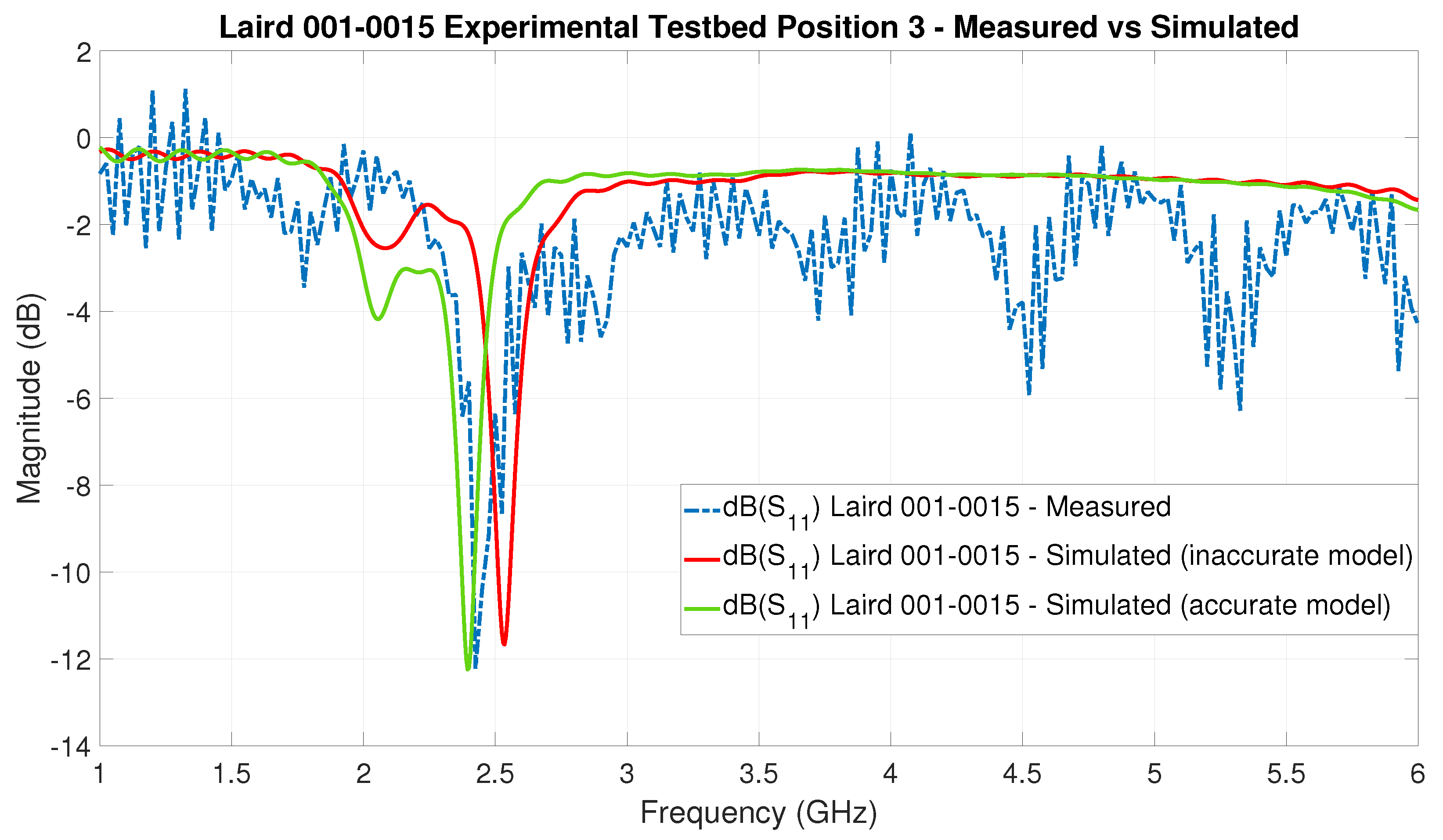
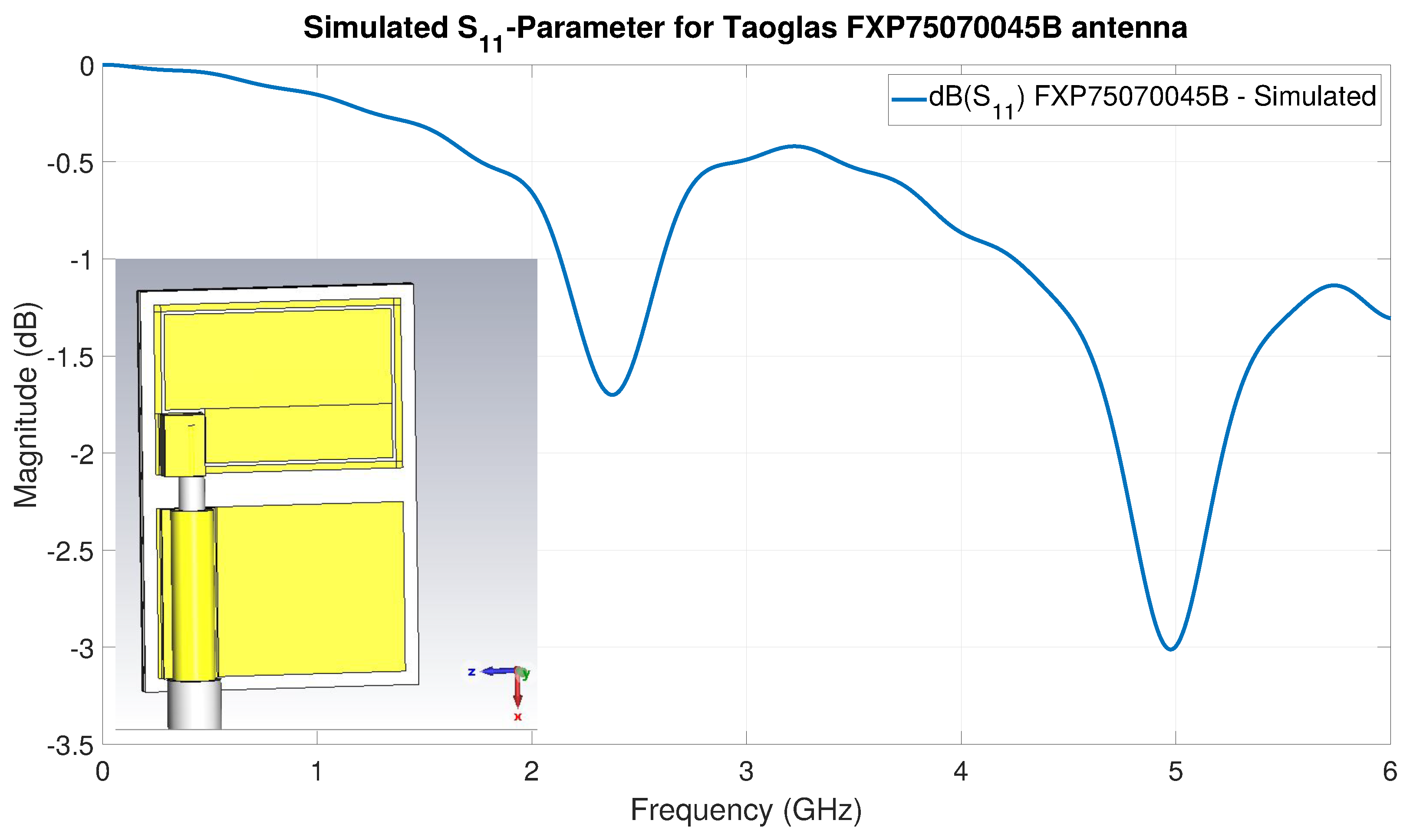
6.4. S Parameters EM Simulation versus VNA
6.5. Heterogeneous Antenna Setup
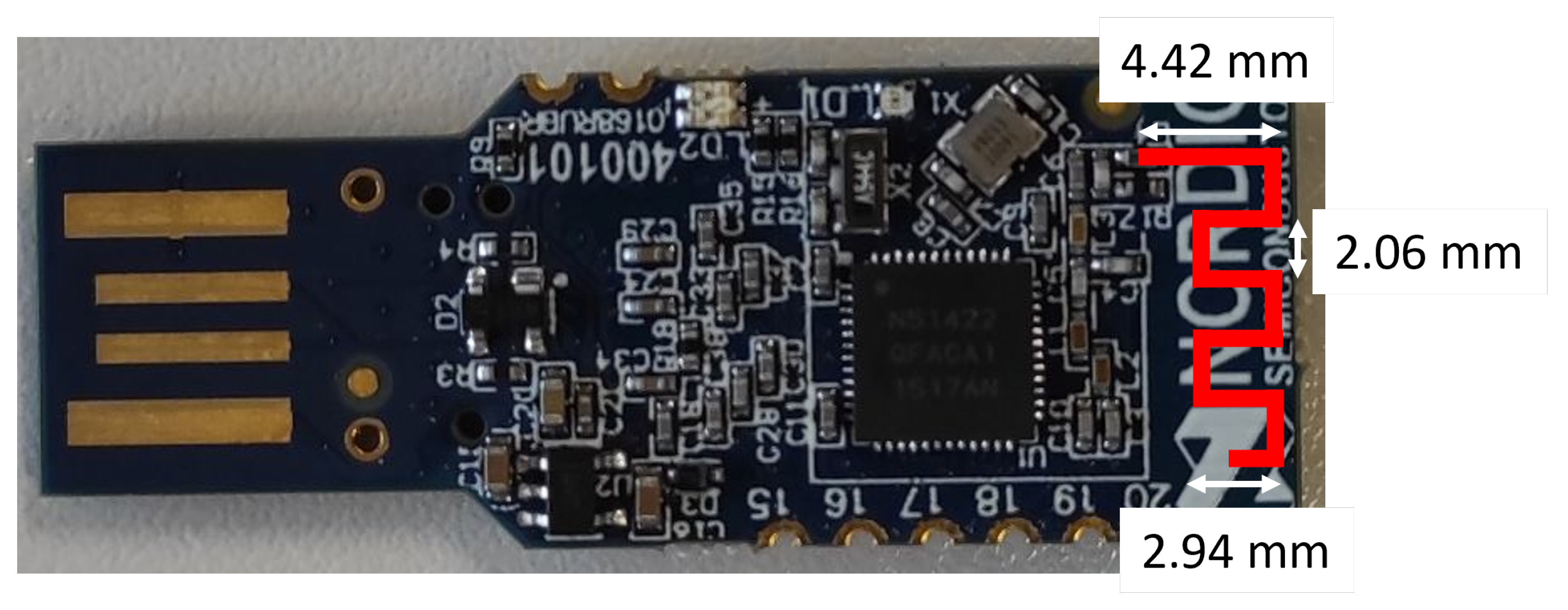
6.6. Electromagnetic Antenna Modeling
6.7. Ray-Tracing Simulation Results
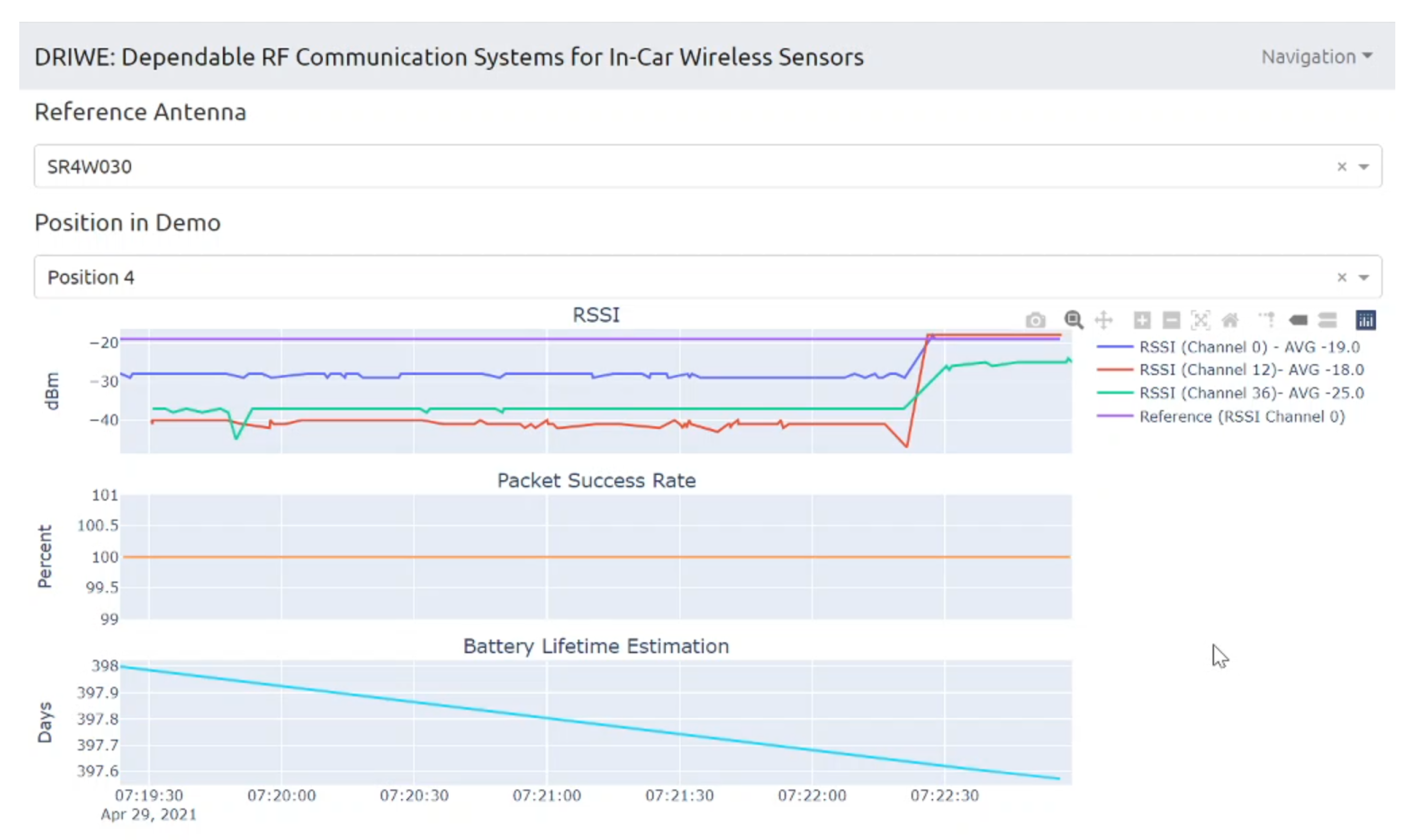
6.8. Prototype Antenna-Recommender System
7. Lessons Learned
8. Future Work
9. Conclusions
Author Contributions
Funding
Institutional Review Board Statement
Informed Consent Statement
Data Availability Statement
Acknowledgments
Conflicts of Interest
References
- Kraus, D.; Ivanov, H.; Leitgeb, E. Approach for an Optical Network Design for Autonomous Vehicles. In Proceedings of the 2019 21st International Conference on Transparent Optical Networks (ICTON), Angers, France, 9–13 July 2019; pp. 1–6. [Google Scholar]
- Munir, S.A.; Ren, B.; Jiao, W.; Wang, B.; Xie, D.; Ma, J. Mobile Wireless Sensor Network: Architecture and Enabling Technologies for Ubiquitous Computing. In Proceedings of the 21st International Conference on Advanced Information Networking and Applications Workshops (AINAW’07), Niagara Falls, ON, Canada, 21–23 May 2007; Volume 2, pp. 113–120. [Google Scholar]
- Chowdhury, S.; Frolik, J.; Benslimane, A. Polarization Matching for Networks Utilizing Tripolar Antenna Systems. In Proceedings of the 2018 IEEE Global Communications Conference (GLOBECOM), Abu Dhabi, United Arab Emirates, 9–13 December 2018; pp. 206–212. [Google Scholar]
- Shahid, N.; Naqvi, I.; Qaisar, S. Characteristics and Classification of Outlier Detection Techniques for Wireless Sensor Networks in Harsh Environments: A Survey. Artif. Intell. Rev. 2012, 43, 193–228. [Google Scholar] [CrossRef]
- Mazuelas, S.; Lorenzo, R.M.; Bahillo, A.; Fernandez, P.; Prieto, J.; Abril, E. Topology Assessment Provided by Weighted Barycentric Parameters in Harsh Environment Wireless Location Systems. IEEE Trans. Signal Process. 2010, 58, 3842–3857. [Google Scholar] [CrossRef]
- Di Renzo, M.; Debbah, M.; Phan-Huy, D.; Zappone, A.; Alouini, M.; Yuen, C.; Sciancalepore, V.; Alexandropoulos, G.; Hoydis, J.; Gacanin, H.; et al. Smart Radio Environments Empowered by Reconfigurable AI Meta-Surfaces: An idea whose time has come. EURASIP J. Wirel. Commun. Netw. 2019, 129, 1–20. [Google Scholar] [CrossRef]
- Mitzlaff, J. Radio Propagation and Anti-Multipath Techniques in the WIN Environment. IEEE Netw. 1991, 5, 21–26. [Google Scholar] [CrossRef]
- Croonenbroeck, R.; Underberg, L.; Wulf, A.; Kays, R. Measurements for the Development of an Enhanced Model for Wireless Channels in Industrial Environments. In Proceedings of the 2017 IEEE 13th International Conference on Wireless and Mobile Computing, Networking and Communications (WiMob), Rome, Italy, 9–11 October 2017; pp. 1–8. [Google Scholar]
- Lin, J.; Talty, T.; Tonguz, O. An Empirical Performance Study of Intra-vehicular Wireless Sensor Networks under WiFi and Bluetooth Interference. In Proceedings of the 2013 IEEE Global Communications Conference (GLOBECOM), Atlanta, GA, USA, 9–13 December 2013; pp. 581–586. [Google Scholar]
- Kraus, D.; Priller, P.; Diwold, K.; Leitgeb, E. Achieving Robust and Reliable Wireless Communications in Hostile In-Car Environments. In Proceedings of the 9th International Conference on the Internet of Things, IoT 2019, Granada, Spain, 22–25 October 2019; p. 4. [Google Scholar]
- Kraus, D.; Diwold, K.; Leitgeb, E. Poster: RSSI-Based Antenna Evaluation for Robust BLE Communication in in-Car Environments. In Proceedings of the 2021 International Conference on Embedded Wireless Systems and Networks, Delft, The Netherlands, 17–19 February 2021; pp. 167–168. [Google Scholar]
- Habib, S.; Hannan, M.; Javadi, M.; Samad, S.; Muad, A.; Hussain, A. Inter-Vehicle Wireless Communications Technologies, Issues and Challenges. Inf. Technol. J. 2013, 12, 558–568. [Google Scholar]
- Parthasarathy, D.; Whiton, R.; Hagerskans, J.; Gustafsson, T. An In-Vehicle Wireless Sensor Network for Heavy Vehicles. In Proceedings of the 2016 IEEE 21st International Conference on Emerging Technologies and Factory Automation (ETFA), Berlin, Germany, 6–9 September 2016; pp. 1–8. [Google Scholar]
- IETF. IPv6 over the TSCH Mode of IEEE 802.15.4e (6tisch). 2018. Available online: https://datatracker.ietf.org/wg/6tisch/charter/ (accessed on 8 October 2021).
- Yusoff, I.; Peng, X. Impacts of Channel Loss and Electromagnetic Interference on Intra-Vehicle Wireless Communications. In Proceedings of the 2020 IEEE 91st Vehicular Technology Conference (VTC2020-Spring), Antwerp, Belgium, 25–28 May 2020; pp. 1–5. [Google Scholar]
- Balachander, D.; Rao, T.; Tiwari, N. In-Vehicle RF Propagation Measurements for Wireless Sensor Networks at 433/868/915/2400MHz. In Proceedings of the 2013 International Conference on Communication and Signal Processing, Melmaruvathur, India, 3–5 April 2013; pp. 419–422. [Google Scholar]
- Großwindhager, B.; Rath, M.; Bakr, M.; Greiner, P.; Boano, C.; Witrisal, K.; Gentili, F.; Grosinger, J.; Bösch, W.; Römer, K. Dependable Wireless Communication and Localization in the Internet of Things. In Mission-Oriented Sensor Networks and Systems: Art and Science: Volume 2: Advances; Springer: Berlin, Germany, 2019; pp. 209–256. [Google Scholar]
- Khan, H.; Grosinger, J.; Auinger, B.; Amschl, D.; Priller, P.; Muehlmann, U.; Bösch, W. Measurement Based Indoor SIMO RFID Simulator for Tag Positioning. In Proceedings of the 2015 International EURASIP Workshop on RFID Technology (EURFID), Rosenheim, Germany, 22–23 October 2015; pp. 112–119. [Google Scholar]
- Saxl, G.; Görtschacher, L.; Ussmueller, T.; Grosinger, J. Software-Defined RFID Readers: Wireless Reader Testbeds Exploiting Software-Defined Radios for Enhancements in UHF RFID Systems. IEEE Microw. Mag. 2021, 22, 46–56. [Google Scholar] [CrossRef]
- Song, H.; Hsu, H.; Wiese, R.; Talty, T. Modeling Signal Strength Range of TPMS in Automobiles. IEEE Antennas Propag. Soc. Symp. 2004, 3, 3167–3170. [Google Scholar]
- Zeng, H.; Hubing, T. The Effect of the Vehicle Body on EM Propagation in Tire Pressure Monitoring Systems. IEEE Trans. Antennas Propag. 2012, 60, 3941–3949. [Google Scholar] [CrossRef]
- Lasser, G.; Langwieser, R.; Xaver, F.; Mecklenbräuker, C. Dual-Band Channel Gain Statistics for Dual-Antenna Tyre Pressure Monitoring RFID Tags. In Proceedings of the 2011 IEEE International Conference on RFID, Sitges, Spain, 15–16 September 2011; pp. 57–61. [Google Scholar]
- Choudhury, B.; Singh, H.; Bommer, J.; Jha, R. RF Field Mapping Inside a Large Passenger-Aircraft Cabin Using a Refined Ray-Tracing Algorithm. IEEE Antennas Propag. Mag. 2013, 55, 276–288. [Google Scholar] [CrossRef]
- Felbecker, R.; Keusgen, W.; Peter, M. Incabin Millimeter Wave Propagation Simulation in a Wide-Bodied Aircraft Using Ray-Tracing. In Proceedings of the 2008 IEEE 68th Vehicular Technology Conference, Calgary, AB, Canada, 21–24 September 2008; pp. 1–5. [Google Scholar]
- Kraus, D.; Diwold, K.; Leitgeb, E. Getting on Track—Simulation-aided Design of Wireless IoT Sensor Systems. In Proceedings of the 2020 International Conference on Broadband Communications for Next Generation Networks and Multimedia Applications (CoBCom), Graz, Austria, 12–14 July 2020; pp. 1–6. [Google Scholar]
- Yun, Z.; Iskander, M. Ray Tracing for Radio Propagation Modeling: Principles and Applications. IEEE Access 2015, 3, 1089–1100. [Google Scholar] [CrossRef]
- Fuschini, F.; Barbiroli, M.; Zoli, M.; Bellanca, G.; Calò, G.; Bassi, P.; Petruzzelli, V. Ray Tracing Modeling of Electromagnetic Propagation for On-Chip Wireless Optical Communications. J. Low Power Electron. Appl. 2018, 8, 39. [Google Scholar] [CrossRef]
- Francisco, R.; Huang, L.; Dolmans, G.; Groot, H. Coexistence of ZigBee Wireless Sensor Networks and Bluetooth Inside a Vehicle. In Proceedings of the 2009 IEEE 20th International Symposium on Personal, Indoor and Mobile Radio Communications, Tokyo, Japan, 13–16 September 2009; pp. 2700–2704. [Google Scholar]
- Yun, D.; Lee, S.; Kim, D. A Study on the Vehicular Wireless Base-Station for In-Vehicle Wireless Sensor Network System. In Proceedings of the 2014 International Conference on Information and Communication Technology Convergence (ICTC), Busan, Korea, 22–24 October 2014; pp. 609–610. [Google Scholar]
- Firmansyah, E.; Grezelda, L. RSSI Based Analysis of Bluetooth Implementation for Intra-Car Sensor Monitoring. In Proceedings of the 2014 6th International Conference on Information Technology and Electrical Engineering (ICITEE), Yogyakarta, Indonesia, 7–8 October 2014; pp. 1–5. [Google Scholar]
- Herbert, S.; Wassell, I.; Loh, T.; Rigelsford, J. Characterizing the Spectral Properties and Time Variation of the In-Vehicle Wireless Communication Channel. IEEE Trans. Commun. 2014, 62, 2390–2399. [Google Scholar] [CrossRef]
- Takayama, I.; Kajiwara, A. Intra-Vehicle Wireless Harness with Mesh-Networking. In Proceedings of the 2016 IEEE-APS Topical Conference on Antennas and Propagation in Wireless Communications (APWC), Cairns, Australia, 19–23 September 2016; pp. 146–149. [Google Scholar]
- Sharma, R.; Senapati, A.; Roy, J.S. Beamforming of smart antenna in cellular network using leaky LMS algorithm. In Proceedings of the 2018 Emerging Trends in Electronic Devices and Computational Techniques (EDCT), Kolkata, India, 8–9 March 2018; pp. 1–5. [Google Scholar]
- Prerna Saxena, A.G. Kothari, Performance Analysis of Adaptive Beamforming Algorithms for Smart Antennas. IERI Procedia 2014, 10, 131–137. [Google Scholar] [CrossRef]
- Bhoyar, D.B.; Dethe, C.G.; Mushrif, M.M.; Narkhede, A.P. Leaky least mean square (LLMS) algorithm for channel estimation in BPSK-QPSK-PSK MIMO-OFDM system. In Proceedings of the 2013 International Mutli-Conference on Automation, Computing, Communication, Control and Compressed Sensing (iMac4s), Kottayam, India, 22–23 March 2013; pp. 623–629. [Google Scholar]
- Wertz, P.; Cvijic, V.; Hoppe, R.; Wolfle, G.; Landstorfer, F. Wave Propagation Modeling Inside Vehicles by Using a Ray Tracing Approach. In Proceedings of the Vehicular Technology Conference, IEEE 55th Vehicular Technology Conference, VTC Spring 2002 (Cat. No. 02CH37367), Birmingham, AL, USA, 6–9 May 2002; Volume 3, pp. 1264–1268. [Google Scholar]
- Sun, H.; Wang, J.; Shen, G.; Hu, P. Application of Warm Forming Aluminum Alloy Parts for Automotive Body Based on Impact. Int. J. Automot. Technol. 2013, 14, 605–610. [Google Scholar] [CrossRef]
- Airoldi Metalli. Product Sheet Aluminium Alloy 5754. 2018. Available online: https://www.airoldimetalli.com/wp-content/uploads/2018/05/5754LAM_ENG.pdf (accessed on 24 January 2022).
- Remley, K.; Koepke, G.; Holloway, C.; Camell, D.; Grosvenor, C. Measurements in Harsh RF Propagation Environments to Support Performance Evaluation of Wireless Sensor Networks. Sens. Rev. 2009, 29, 211–222. [Google Scholar] [CrossRef]
- Shi, D.; Tang, X.; Wang, C. The Acceleration of the Shooting and Bouncing Ray Tracing Method on GPUs. In Proceedings of the 2017 XXXIInd General Assembly and Scientific Symposium of the International Union of Radio Science (URSI GASS), Montreal, QC, Canada, 19–26 August 2017; pp. 1–3. [Google Scholar]
- Araujo, M.T.M. A45 Carbon Edition 2017. 2018. Available online: https://grabcad.com/library/a45-carbon-edition-2017-1 (accessed on 20 December 2021).
- Nordic Semiconductor. nRF52840 DK Characterization. 2018. Available online: https://devzone.nordicsemi.com/f/nordic-q-a/37624/nrf52-dk-bluetooth-radiation-diagram/327598#327598 (accessed on 6 September 2021).
- Gao, V. Bluetooth Blog: Proximity and RSSI. 2015. Available online: https://www.bluetooth.com/blog/proximity-and-rssi/ (accessed on 16 June 2021).
- Nordic Semiconductor. nRF52840 Product Specification v1.2. 2021. Available online: https://infocenter.nordicsemi.com/pdf/nRF52840_PS_v1.2.pdf (accessed on 25 August 2021).
- Nordic Semiconductor. nRF5 SDK v17.0.2. 2021. Available online: https://www.nordicsemi.com/Products/Development-software/nrf5-sdk/download (accessed on 25 August 2021).
- Wong, J. BLE Throughput Test with PER. 2019. Available online: https://github.com/jimmywong2003/nrf5-packet-error-rate-measurement-on-ble-connection (accessed on 18 August 2021).
- Nordic Semiconductor. nRF52840 DK User Guide v1.0.0. 2020. Available online: https://infocenter.nordicsemi.com/pdf/nRF52840_DK_User_Guide_20201203.pdf (accessed on 24 August 2021).
- Linx Technologies. Adapter, SMA Plug (Male Pin) to MHF Jack (Male Pin), ADP-SMAM-UFLF. 2019. Available online: https://www.mouser.at/datasheet/2/238/adp-smam-uflf-1633258.pdf (accessed on 25 August 2021).
- Hirose Electric Co., Ltd. CL331-0472-2-01, U.FL-R-SMT-1(01). 2021. Available online: https://www.hirose.com/de/product/document?clcode=CL0331-0472-2-01&productname=U.FL-R-SMT-1(01)&series=U.FL&documenttype=SpecSheet&lang=de&documentid=0000266605 (accessed on 29 October 2021).
- Cinch Connectivity Solutions. SMA 50 Ohm End Launch Jack Receptacle—Round Contact, 142-0701-801. 2001. Available online: https://www.belfuse.com/resources/productinformations/cinchconnectivitysolutions/johnson/pi-ccs-john-142-0701-801.pdf (accessed on 28 October 2021).
- Bluetooth Special Interest Group (SIG). Bluetooth Core Specification Version 5.2. 2019. Available online: https://www.bluetooth.org/docman/handlers/downloaddoc.ashx?doc_id=478726 (accessed on 18 August 2021).
- Antenova Limited SR4W030-PS-1.2, Zenon 2.4GHz Antenna. 2019. Available online: https://www.antenova.com/wp-content/uploads/2020/05/Zenon-SR4W030-PS-1.2.pdf?hsCtaTracking=b731b9be-15c5-4cd7-b86f-18200b74688c%7C3bc2b3bf-2e06-4022-85f4-543c61946ba4 (accessed on 27 October 2021).
- KYOCERA AVX. Part No. 1001932PT, WLAN/BT/Zigbee Tunable Embedded PCB Antenna. 2021. Available online: https://datasheets.kyocera-avx.com/ethertronics/AVX-E_1001932PT.pdf (accessed on 28 October 2021).
- KYOCERA AVX. Part No. 1000418, WLAN/BT/Zigbee Embedded Stamped Metal Antenna. 2021. Available online: https://datasheets.kyocera-avx.com/ethertronics/AVX-E_1000418.pdf (accessed on 28 October 2021).
- Laird Connectivity. FlexNotch, Adhesive-Backed Flexible Notch Antenna 2400–2500 MHz. 2019. Available online: https://www.lairdconnect.com/documentation/flexnotch-antenna-datasheet-0919 (accessed on 27 October 2021).
- Laird Connectivity. mFlexPIFA, 2.4–2.5 GHz mFlex PIFA +2dBi Antenna. 2021. Available online: https://www.lairdconnect.com/documentation/datasheet-mflexpifapdf (accessed on 27 October 2021).
- Laird Connectivity. NANOBLADE, Internal Wireless Device Antenna 24007–2500 MHz/4900–6000 MHz. 2021. Available online: https://www.lairdconnect.com/documentation/datasheet-nanoblade (accessed on 27 October 2021).
- Laird Connectivity. Mini NanoBlade, Embedded Dual-Band Planar Antenna 2400–2500 MHz/4900–5875 MHz. 2020. Available online: https://www.lairdconnect.com/documentation/datasheet-mini-nanoblade (accessed on 27 October 2021).
- Molex. 2.4/5 GHz Wi-Fi Flexible Antenna with Balanced Transmission. 2015. Available online: https://www.content.molex.com/dxdam/literature/987650-5892.pdf? (accessed on 27 October 2021).
- Molex. Combo Antennas, Wi-Fi 6E+GNSS PCB Cabled Balanced Antenna (Series 146220). 2021. Available online: https://www.content.molex.com/dxdam/2f/2f81553e-80f0-4ddc-9072-009e28c775b8/Combo%20Antennas_DS%20EN%20%5B987651-3851%20rev6%5D.pdf? (accessed on 27 October 2021).
- Molex. 2.4, 5 GHz Flexible and PCB Antennas. 2020. Available online: https://www.content.molex.com/dxdam/13/13192920-5f8a-47ac-9f6d-aa63b0ccfdaf/987651-6901.pdf? (accessed on 28 October 2021).
- PulseLarsen Antennas. FPC Antenna 2.4/5.xGHz/DSRC. 2020. Available online: https://productfinder.pulseelectronics.com/api/open/product-attachments/datasheet/w3334b0150 (accessed on 28 October 2021).
- Taoglas. SPE-12-8-013 - FXP70.07.0053A, 2.4 GHz Freedom Flexible PCB Antenna. 2019. Available online: https://www.taoglas.com/datasheets/FXP70.07.0053A.pdf (accessed on 28 October 2021).
- Taoglas. SPE-12-8-137/F/OH - FXP74.07.0100A, FXP74 Black Diamond 2.4GHz Band Antenna. 2019. Available online: https://www.taoglas.com/datasheets/FXP74.07.0100A.pdf (accessed on 28 October 2021).
- Taoglas. SPE-13-8-067/D/EZ - FXP75.07.0045B, FXP.75 Atom 2.4GHz Series. 2017. Available online: https://www.taoglas.com/datasheets/FXP75.07.0045B.pdf (accessed on 28 October 2021).
- Taoglas. SPE-11-8-050-G - FXP810.07.0100C, FXP810 2.4/4.9-6GHz Dual-band Antenna. 2021. Available online: https://www.taoglas.com/datasheets/FXP810.07.0100C.pdf (accessed on 28 October 2021).
- Taoglas. Specification WCM.01.0151. 2016. Available online: https://www.taoglas.com/datasheets/WCM.01.0151.pdf (accessed on 27 October 2021).
- Tyco Electronics Corporation. 2300–3800 MHz Single Band Antenna, 2118059-1. 2011. Available online: https://www.te.com/commerce/DocumentDelivery/DDEController?Action=showdoc&DocId=Data+Sheet%7F2118059%7FA%7Fpdf%7FEnglish%7FENG_DS_2118059_A.pdf%7F2118059-1 (accessed on 27 October 2021).
- YAGEO Group. PCB Type Antenna ANTX100P001B24003 2.45 GHz. 2014. Available online: https://www.yageo.com/upload/media/product/productsearch/datasheet/wireless/An_PCB_2450_ANTX100P001B24003_v0.pdf (accessed on 28 October 2021).
- YAGEO Group. PCB Type Antenna ANTX100P111B24003 2.40 2.50GHz. 2015. Available online: https://www.yageo.com/upload/media/product/productsearch/datasheet/wireless/An_PCB_2450_ANTX100P111B24003_0.pdf (accessed on 28 October 2021).
- YAGEO Group. PCB Type Antenna ANTX100P113B24003 2.40 2.50GHz. 2016. Available online: https://www.yageo.com/upload/media/product/productsearch/datasheet/wireless/An_PCB_2450_ANTX100P113B24003_0.pdf (accessed on 28 October 2021).
- Telegärtner. SMA Bulkhead Receptacle J01151A0021. 2008. Available online: https://www.telegaertner.com/fileadmin/pdms_files/J01151A0021KP.pdf (accessed on 14 September 2021).
- Molex. BSA SMA Plug to MCRF Plug 50 Ohms BSA-SMAP/MCRFP. 2012. Available online: https://www.molex.com/pdm_docs/sd/733860850_sd.pdf (accessed on 14 September 2021).
- Winters, J.H. Smart antenna techniques and their application to wireless ad hoc networks. IEEE Wirel. Commun. 2006, 13, 77–83. [Google Scholar] [CrossRef]
- Chopra, R.; Lakhmani, R. Design and comparative evaluation of antenna array performance using non blind LMS beamforming algorithms. In Proceedings of the 2017 Progress in Electromagnetics Research Symposium—Fall (PIERS—FALL), Singapore, 19–22 November 2017; pp. 1827–1834. [Google Scholar]
- Albagory, Y.; Alraddady, F. An Efficient Approach for Sidelobe Level Reduction Based on Recursive Sequential Damping. Symmetry 2021, 13, 480. [Google Scholar] [CrossRef]


| References | Design Strategy | Devices | Protocol/ Frequency | Data/Sample Rate | Investigated Range | Metal Nearby |
|---|---|---|---|---|---|---|
| [20] | Tire-pressure monitoring system (TPMS) | Valve stem (TX) Printed monopole (RX) | 315 MHz | n/s | Up to 1.6 m | Yes |
| [21] | Vehicle body effect on TPMS | TPMS with whip, Loop antennas | 310/433 MHz | n/s | Up to 3 m | Yes |
| [22] | Tire-pressure monitoring RFID tags | Dipole/monopole antennas RFID reader and tags VNA | UHF 866 MHz ISM 2.45 GHz | n/s | Up to 2 m | Yes |
| [28] | Coexistence Zigbee and BLE | CC2520 Zigbee CN512 Bluetooth | Zigbee, BT 2.4 GHz | 250 kbps 1, 2, 3 Mbps | Up to 3 m | Yes |
| [29] | Wireless base station for in-vehicle network | CC2520 Zigbee CC2540 Bluetooth | Zigbee, BT 4 2.4 GHz | 250 kbps 1 Mbps | Up to 3 m | Yes |
| [30] | RSSI-based analysis for intra-car sensor monitoring | HC-05 BT module Smartphone | Bluetooth (BT) 2.4 GHz | 38,400 bps | Up to 4 m | Yes |
| [13,14] | WSNs in heavy vehicles | JN5168 USB dongle | IETF 6TISCH, 2.4 GHz | 250 kbps | Up to 6 m | Yes |
| [16] | RF propagation measurements | Agilent N5182A Agilent N9010A | 433/868/915/ 2400 MHz | 1 Msps | Up to 2.3 m | No |
| [15] | Channel loss measurements | USRP B210 | Zigbee, BT 5, Wi-Fi 2.4 GHz | 20 Msps | Up to 3 m | No |
| [31] | Characterization of the in-vehicle wireless channel | Agilent E4440A, Schwarzbeck 9113 antenna | 2.45 GHz | n/s | Less than 2 m | No |
| [32] | UWB-IR measurements in in-vehicle scenario | Agilent 8722ET | UWB 3-10 GHz | n/s | Up to 3 m | No |
| This work | Antenna recommendation of COTS devices in harsh environments | nRF51/52 dongle nRF52840 DK R&S ZVA24 | Bluetooth Low Energy (BLE 5.0) 2.4 GHz | 1 Mbps | Up to 2 m | Yes |
| Parameter | Setting | Value |
|---|---|---|
| Mode | Field Sources | * |
| Frequency sweep | Frequency range | 2 to 3 GHz |
| Custom Accuracy | Max. intersections | 4 |
| Ray Storage | Visualization options | Show Rays trapped in structure |
| Parameter | Symbol | Value |
|---|---|---|
| Modulation Type | GFSK | data |
| Bit Rate | 1 Mbit/s | |
| Bandwidth | B | 2 MHz |
| Transmission Power | 0 dBm | |
| Frequency Range | 2.402 GHz to 2.48 GHz | |
| Frequency (Advertising Mode) | CH 37: 2.402 GHz, CH 38: 2.426 GHz | |
| CH 39: 2.480 GHz | ||
| Frequency (Connection Mode) | CH 0–39: 2.402 GHz–2.480 GHz | |
| Antenna Gain | G | antenna specific (in dBm) * |
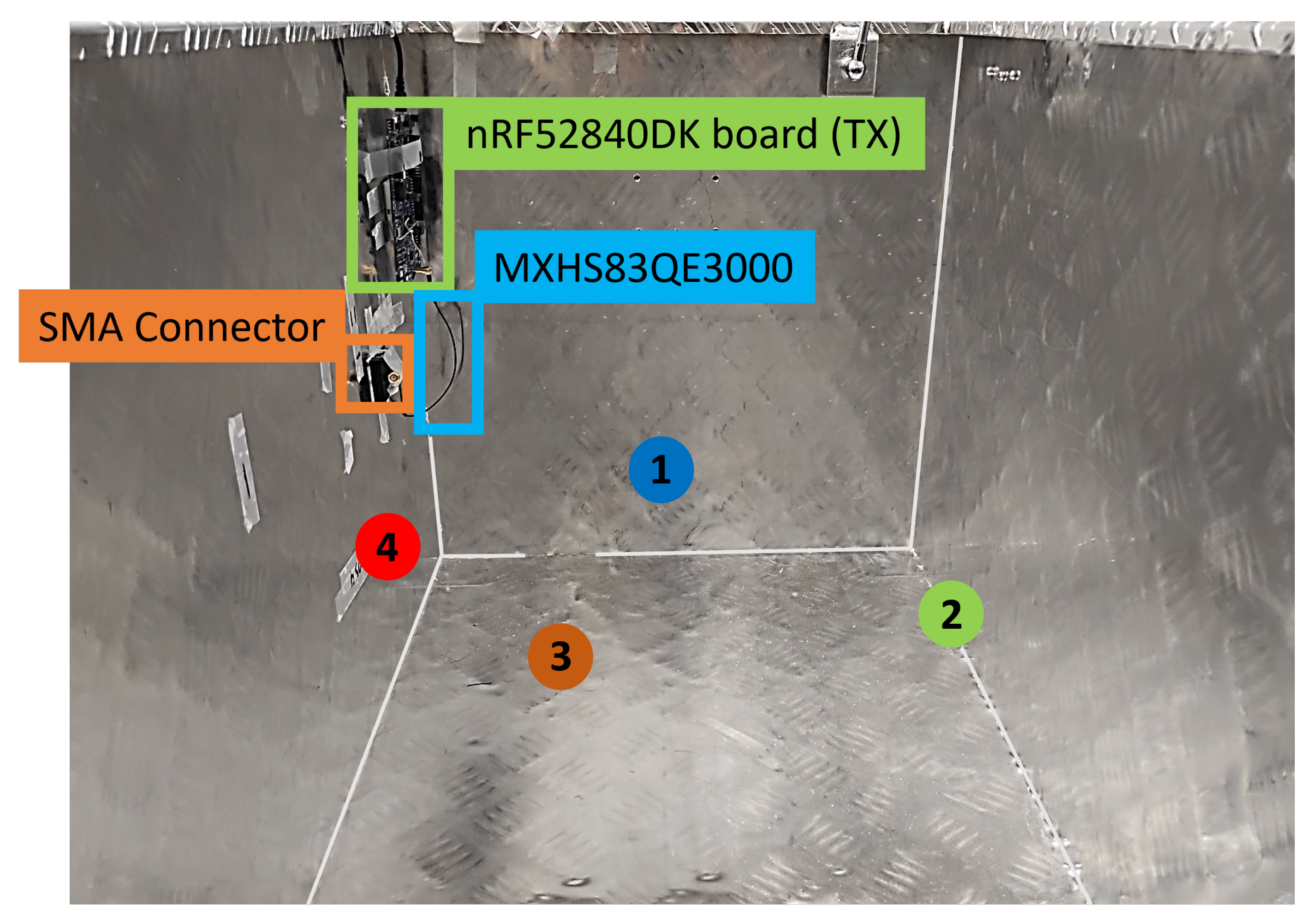
| TX/RX Position | Description |
|---|---|
| TX Position 1 | nRF52840DK board and antenna parallel to left side panel. Located 5.725 cm above inside bottom; 17.8 cm from back-side panel; and 9.25 cm from left side panel. Free space scenario, no metallic object in near field. Emitting radiation of TX is directed towards RX. Direct communication path in range of 60–90° in horizontal plane (see Figure 8) where gain of antenna is close to maximum. |
| TX Position 2 | nRF52840DK board and antenna parallel to left side panel. Located 5.725 cm above the inside bottom; directly adjacent to back-side panel; 9.25 cm from left side panel. main direction of radiation of antenna towards the center of the box. Near field of the antenna influenced by backside panel. This position is used to investigate impact on onboard antenna and external antennas. |
| TX Position 3 | nRF52840DK board and antenna rotated 90° and normal to left side panel. Located 5.7 cm above inside bottom; 26 cm from front panel; 9 cm from left side panel. vertical radiation plane for investigation of differences in radiation efficiency according to Figure 8 and Figure 9. Position 3 to investigate antenna performance in vertical plane. External antennas 20 cm from left side panel; 5 cm above bottom (no impact on near field). |
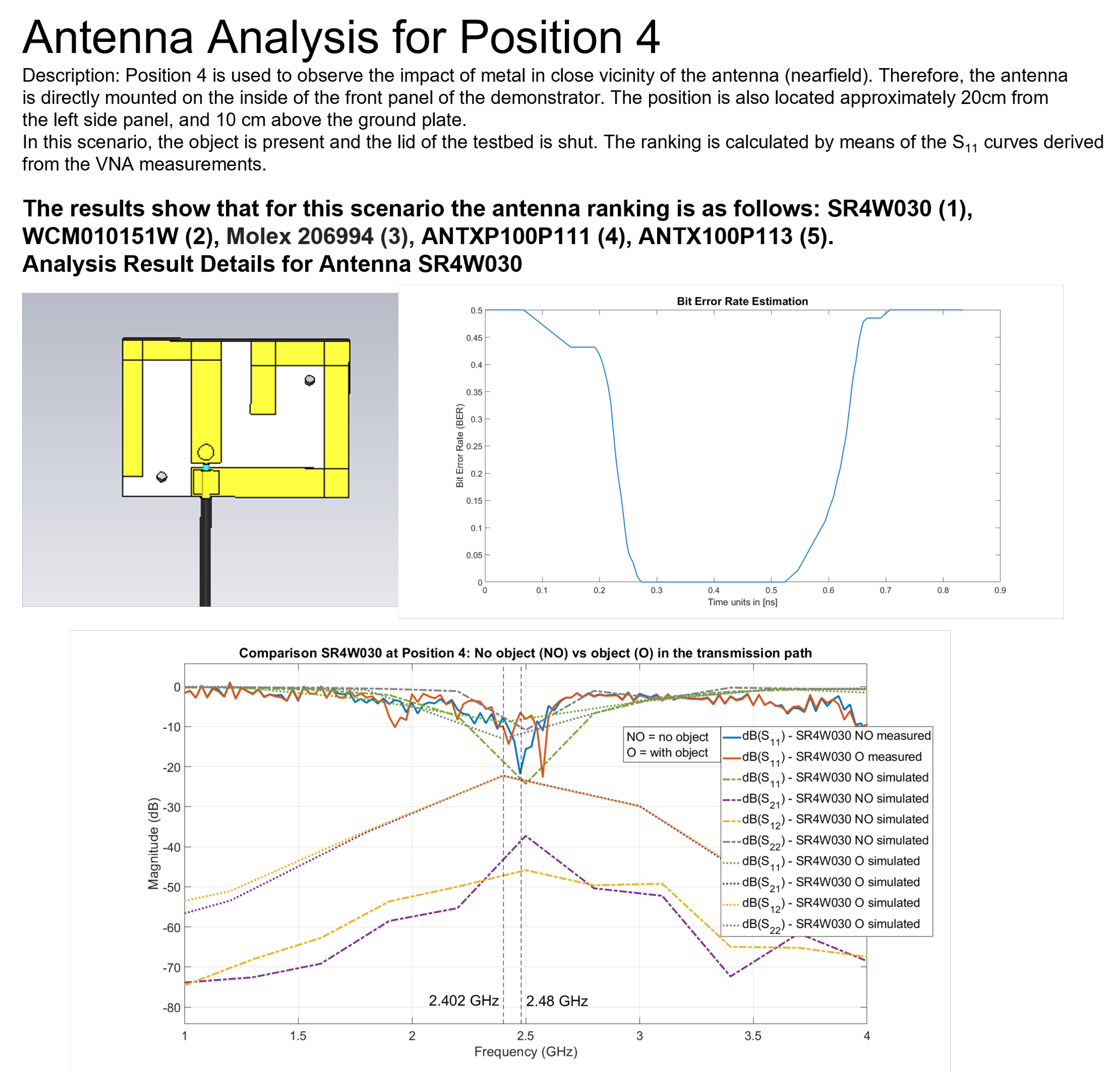
| TX Position 4 | nRF52840DK board and antenna rotated 180°. Located 5.725 cm above inside bottom; 9.25 cm from the left side panel; directly adjacent to front panel. Focus of investigation horizontal plane. Position 4 used to observe impact of metal in near field of antenna. Antenna directly mounted on the inside of front panel. External antenna position: 20 cm from left side panel; 10 cm above bottom plate. |
| RX Position | RX position stationary (see Figure 2): envisaged system with star topology and central receiver in dashboard. RX is nRF52840 DK board with onboard monopole antenna. Main direction of radiation of antenna aimed at center of testbed. Here (angle of approx. 90°), radiation efficiency is close to maximum in horizontal plane. |
| Manufacturer | Antenna Designation |
|---|---|
| Nordic | (1) Monopole nRF52840 DK [47] |
| Antenova | (1) SR4W030 [52] |
| Kyocera AVX | (1) 1001932PT-AA10L0100 [53]; (2) 1000418 Wi-Fi Dual Band [54] |
| Laird | (1) 001-0015 [55]; (2) 001-0034 [56]; (3) CAF94505 [57]; (4) MAF94264 [58] |
| Molex | (1) 47950-4011 [59]; (2) 146220-0100 [60]; (3) 204281-0100 [61]; (4) 206994-0100 [61] |
| Pulse Larsen | (1) W3334B0150 [62] |
| Taoglas | (1) FXP70070053A [63]; (2) FXP74070100A [64]; (3) FXP75070045B [65]; (4) FXP810070100C [66]; (5) WCM010151W [67] |
| TE Connectivity | (1) 2118059-1 [68] |
| Yageo | (1) ANTX100P001B24003 [69]; (2) ANTX100P111B24003 [70]; (3) ANTX100P113B24003 [71] |
| Position | Result Description |
|---|---|
| Position 1 | Position reflects undisturbed communication scenario; antenna is radiating in angle with highest gain. Towards receiving antenna. Expected results: antennas work as stated in their data sheets. Achieved results: majority of antennas worked as expected (shown with RSSI and VNA measurements). Antennas with offset had to be matched with adapter implementation (see Section 5.3). Antennas that required matching: AVX 1001932PT-AA10L0100, Taoglas FXP70070053A. |
| Position 2 | Metal in near field of antenna. Antennas aligned for maximum directivity towards receiving antenna. Expected results: some antennas might show frequency shift or will not work when close to metal. Achieved results: many antennas exhibit weakness (as expected) when close to the metal surface (checked with RSSI and VNA measurements). Antennas that performed well: TE Connectivity 2118059-1, Antenova SR4W030, Laird CAF94505, Molex 146220-0100. |
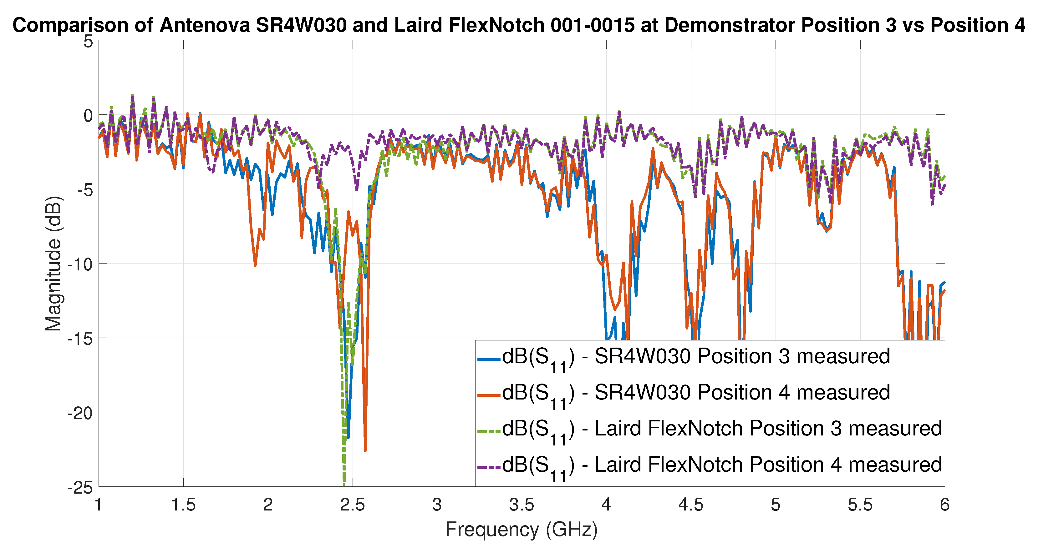
| Position 3 | Position reflects the undisturbed communication scenario. Expected results: reflects the general antenna. Behavior at the defined frequency. Transmission characteristics similar to free space (no near field impact). Achieved results: antennas behave as expected and performance can be derived from the free space scenario. Results are very similar to the ones achieved at position 1. |
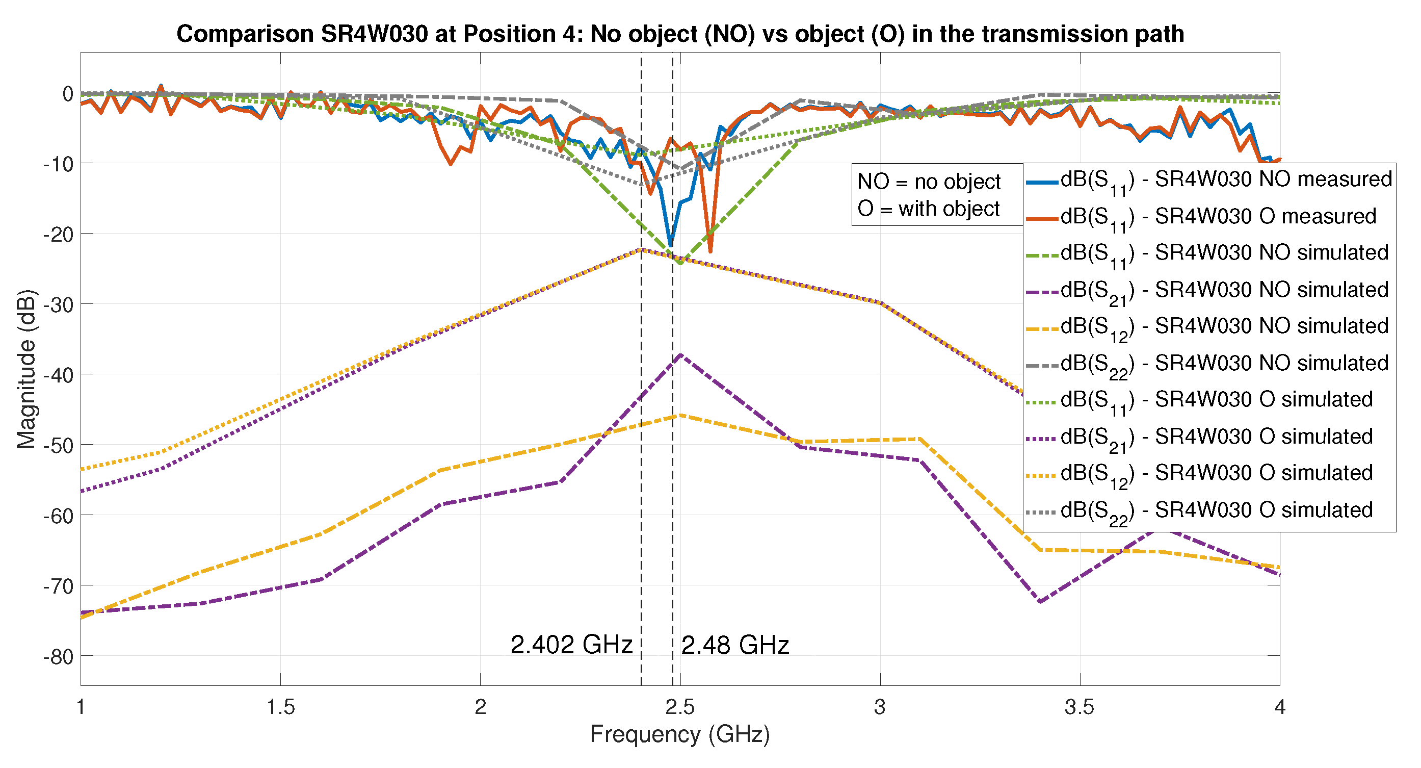
| Position 4 | Metal is in or close to the near field of the antenna. Expected results: impact of metal in near field of antennas revealed. Achieved results: some antennas work considerably well, other antennas lose their characteristics and are not suitable for operation anymore. Based on the results: Some antennas can be omitted for positions close to metal in the testbed. However, these antennas might work good for positions with distance to metal. Antennas that performed well: Antenova SR4W030, Yageo ANTXP100P113, Yageo ANTX100P111, TE Connectivity 2118059-1, Taoglas WCM010151W. |
| BLE (2.402–2.48 GHz) | RSSI [dBm]: min/avg/max | VNA S-Parameter [dB]: min/avg/max | ||||
|---|---|---|---|---|---|---|
| Antenna | NO-LO | NO-LS | O-LO | O-LS | NO-LS | O-LS |
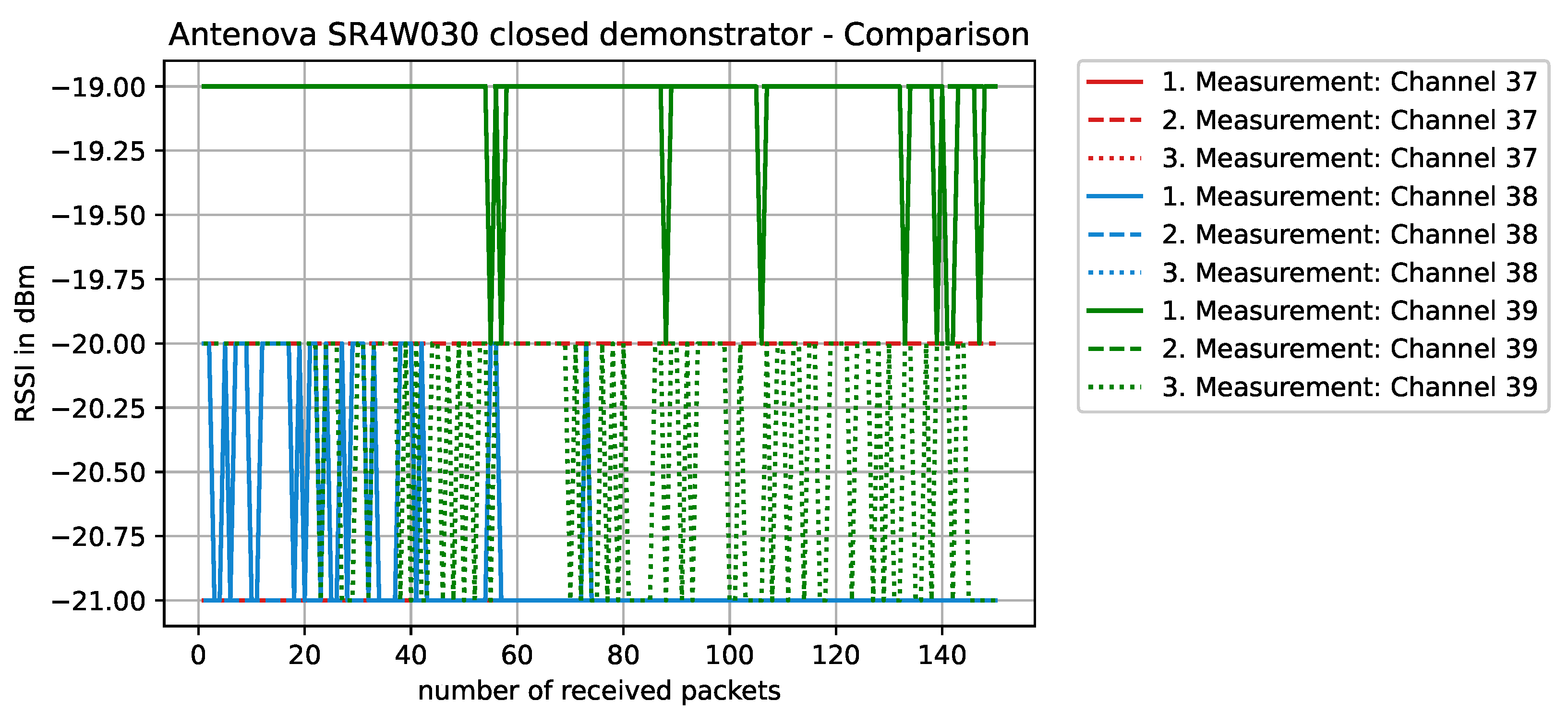
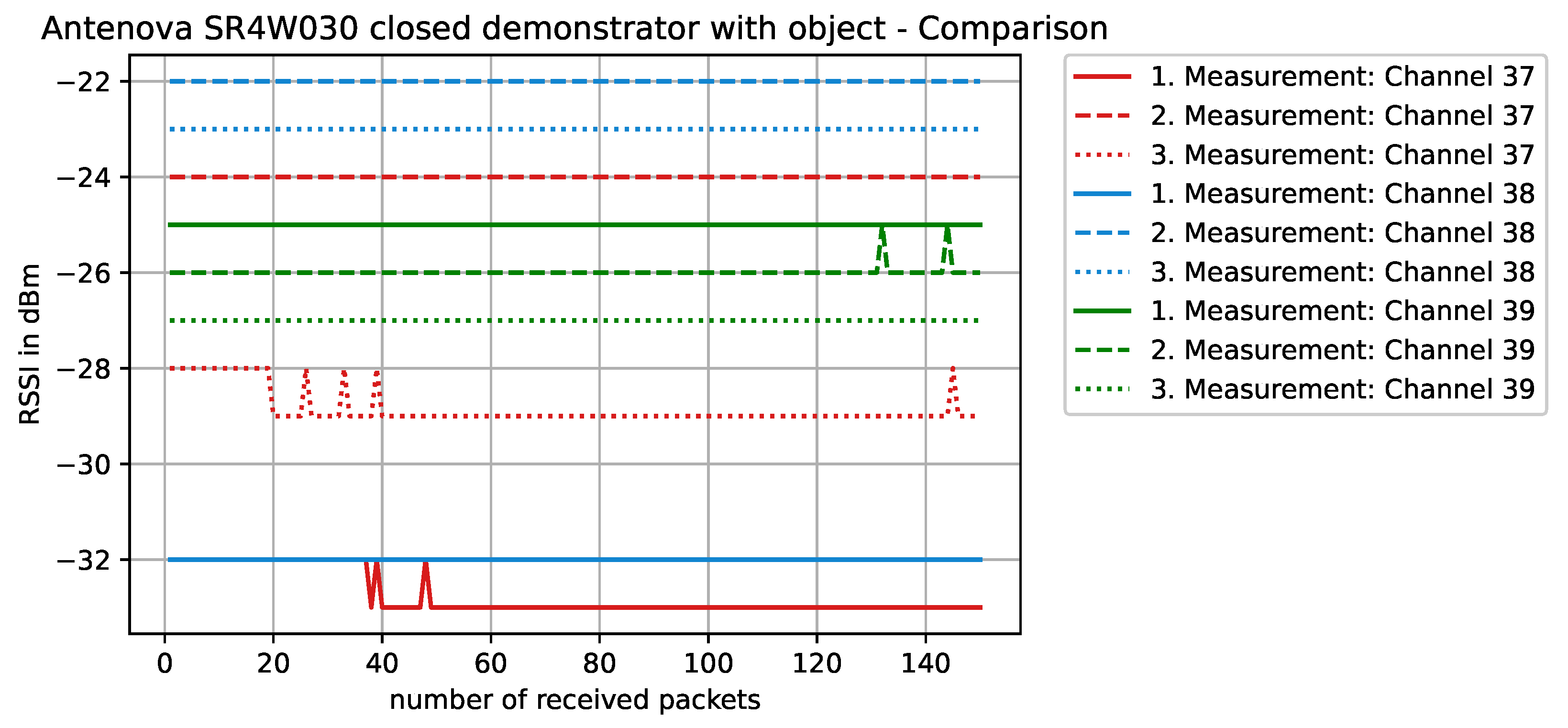
| Antenova SR4W030 | −22/−26/−33 | −19/−20/−21 | −21/−25/−31 | −22/−26/−33 | −8.1/−13.2/−21.9 | −3.4/−7.4/−12.0 |
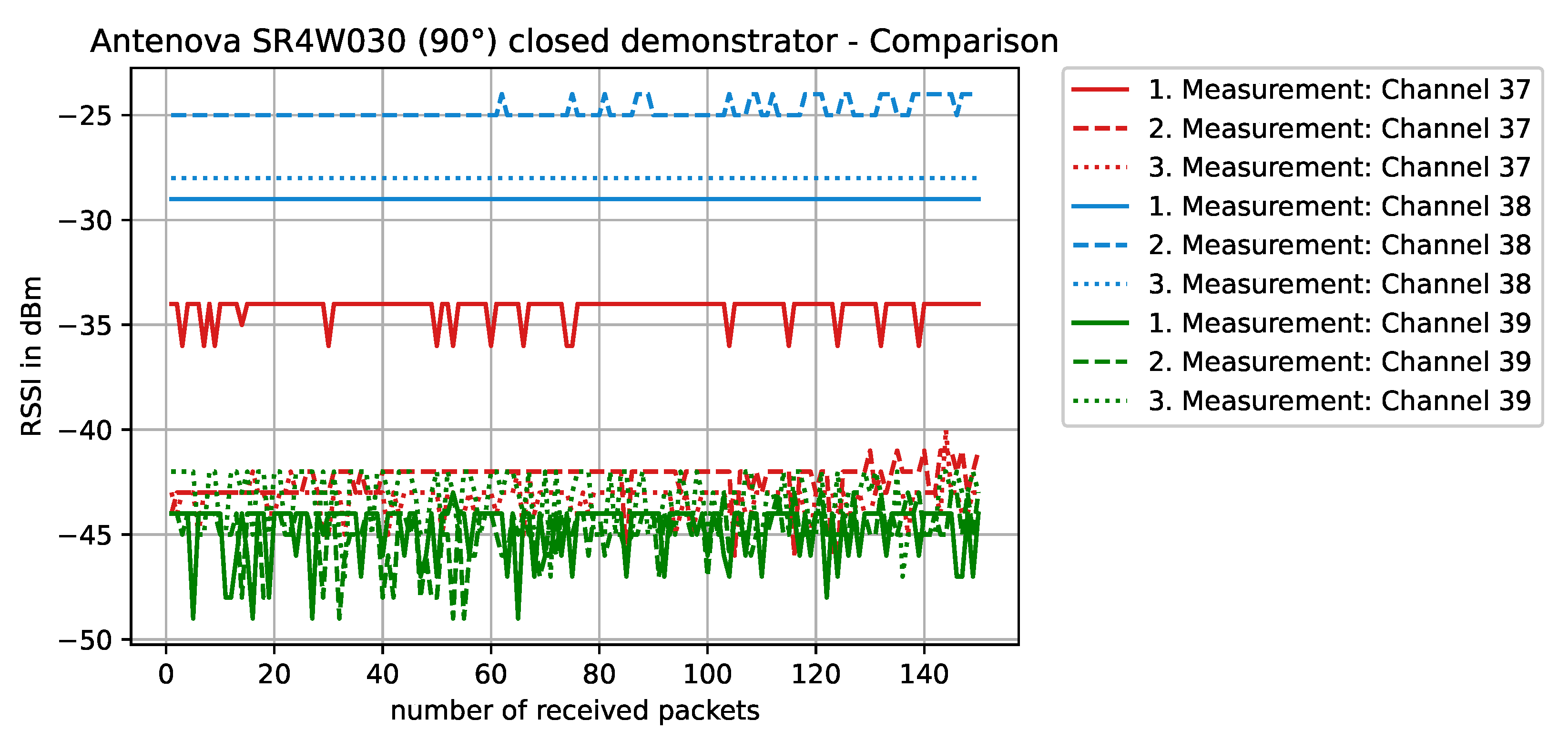
| Antenova SR4W030 | 90° rotation | −24/−36/−48 | 90° rotation | −31/−37/−45 | ||
| Kyocera AVX1000418 | −27/−32/−40 | −19/−25/−33 | −33/−37/−45 | −30/−44/−65 | −9.3/−13.5/−20.3 | −2.1/−3.5/−4.1 |
| Kyocera AVX1001932PT | −22/−32/−43 | −18/−26/−37 | −29/−39/−50 | −26/−37/−53 | −3.9/−7.7/−14.9 | −1.9/−3.1/−3.9 |
| Laird 001-0015 | −18/−33/−58 | −20/−35/−54 | −27/−41/−51 | −26/−38/−50 | −5.9/−10.8/−12.3 | −2.3/−3.6/−5.1 |
| Laird 001-0034 | −25/−29/−33 | −25/−27/−30 | −36/−41/−45 | −38/−43/−50 | −6.1/−9.2/−11.2 | n/a ** |
| Laird CAF94505 | −22/−26/−38 | −19/−25/−36 | −32/−38/−45 | −28/−37/−44 | −4.1/−6.5/−8.4 | −2.1/−2.4/−3.3 |
| Laird MAF94264 | −22/−36/−46 | −20/−30/−42 | −32/−43/−53 | −32/−42/−50 | −5.2/−7.5/−10.0 | −1.8/−2.1/−2.9 |
| Molex 47950 | −33/−36/−47 | −28/−32/−41 | −38/−44/−61 | −34/−43/−49 | – * | – * |
| Molex 146220 | −26/−35/−43 | −24/−35/−51 | −35/−44/−47 | −35/−43/−51 | −4.1/−6.9/−9.0 | −0.8/−1.3/−2.1 |
| Molex 204281 | −29/−37/−50 | −25/−35/−41 | −41/−45/−53 | −34/−44/−50 | n/a ** | n/a ** |
| Molex 206994 | −18/−32/−43 | −23/−35/−61 | −34/−48/−62 | −28/−45/−57 | −5.0/−8.9/−11.3 | −4.5/−5.8/−7.9 |
| Pulse Larsen W3334B0150 | −18/−27/−39 | −17/−30/−45 | −28/−40/−54 | −28/−36/−50 | – * | – * |
| Taoglas FXP70070053A | −17/−21/−27 | −19/−22/−30 | −29/−32/−41 | −26/−30/−41 | −3.2/−4.5/−6.3 | −1.1/−2.3/−3.4 |
| Taoglas FXP74070100A | −20/−33/−46 | −18/−36/−60 | −28/−39/−47 | −30/−41/−51 | −7.2/−9.6/−13.2 | −2.4/−3.3/−4.5 |
| Taoglas FXP75070045B | −26/−32/−45 | −29/−35/−46 | −36/−40/−50 | −31/−43/−55 | −6.8/−9.8/−14.7 | −2.1/−2.8/−3.7 |
| Taoglas FXP810070100C | −29/−33/−42 | −29/−33/−46 | −34/−47/−58 | −35/−46/−58 | −3.8/−5.6/−7.7 | −1.3/−2.2/−2.9 |
| Taoglas WCM010151W | −17/−19/−20 | −17/−19/−21 | −27/−30/−33 | −25/−32/−43 | −6.5/−14.8/−24.2 | −4.3/−7.4/−9.2 |
| Taoglas WCM010151W | 90° rotation | −17/−19/−25 | ||||
| TE Connectivity 2118059 | −22/−30/−40 | −18/−25/−33 | −29/−40/−52 | −25/−39/−53 | −7.8/−12.7/−19.9 | −3.5/−4.7/−5.9 |
| Yageo ANTX100P001 | −17/−23/−27 | −19/−25/−31 | −29/−33/−36 | −26/−30/−36 | −8.8/−9.9/−13.2 | −2.3/−3.1/−4.4 |
| Yageo ANTX100P111 | −17/−20/−28 | −17/−22/−33 | −24/−29/−33 | −24/−26/−30 | −6.2/−12.2/−23.1 | −4.3/−5.6/−7.2 |
| Yageo ANTX100P113 | −17/−24/−31 | −17/−25/−37 | −23/−32/−46 | −25/−30/−34 | −8.1/−11.3/−14.8 | −4.4/−5.2/−6.3 |
| GREEN—Best quality | ||||||
| YELLOW | ||||||
| ORANGE | ||||||
| RED—Worst quality | ||||||
| BLE (2.402–2.48 GHz) | VNA S-Parameter [dB]: min/avg/max | Simulation S-Parameter [dB]: min/avg/max | ||
|---|---|---|---|---|
| Antenna | NO-LS | O-LS | NO-LS | O-LS |
| Antenova SR4W030 | −8.1/−13.2/−21.9 | −3.4/−7.4/−12.0 | −8.3/−14.8/−23.2 | −5.1/−8.2/−9.4 |
| Kyocera AVX1000418 | −9.3/−13.5/−20.3 | −2.1/−3.5/−4.1 | −5.8/−8.4/−12.2 | −2.8/−3.4/−5.1 |
| Kyocera AVX1001932PT | −3.9/−7.7/−14.9 | −1.9/−3.1/−3.9 | −4.4/−7.8/−11.5 | −1.3/−1.7/−2.1 |
| Laird 001-0015 | −5.9/−10.8/−12.3 | −2.3/−3.6/−5.1 | −2.4/−4.6/−6.8 | −1.9/−2.7/−3.7 |
| Laird 001-0034 | −6.1/−9.2/−11.2 | na ** | na ** | na ** |
| Laird CAF94505 | −4.1/−6.5/−8.4 | −2.1/−2.4/−3.3 | −8.1/−9.5/−11.4 | −2.2/−2.5/−3.6 |
| Laird MAF94264 | −5.2/−7.5/−10.0 | −1.8/−2.1/−2.9 | *** | *** |
| Molex 47950 | na * | na * | na * | na * |
| Molex 146220 | −4.1/−6.9/−9.0 | −0.8/−1.3/−2.1 | −2.5/−3.7/−4.5 | −1.2/−1.7/−2.1 |
| Molex 204281 | na ** | na ** | na ** | na ** |
| Molex 206994 | −5.0/−8.9/−11.3 | −4.5/−5.8/−7.9 | −4.2/−6.7/−9.1 | −3.3/−4.7/−6.1 |
| Pulse Larsen W3334B0150 | na * | na * | na * | na * |
| Taoglas FXP70070053A | −3.2/−4.5/−6.3 | −1.1/−2.3/−3.4 | −6.2/−9.6/−12.2 | −1.8/−2.6/−3.2 |
| Taoglas FXP74070100A | −7.2/−9.6/−13.2 | −2.4/−3.3/−4.5 | −13.0/−18.1/−24.3 | −1.4/−1.9/−2.2 |
| Taoglas FXP75070045B | −6.8/−9.8/−14.7 | −2.1/−2.8/−3.7 | *** | *** |
| Taoglas FXP810070100C | −3.8/−5.6/−7.7 | −1.3/−2.2/−2.9 | −2.3/−4.2/−6.5 | −2.1/−2.3/−2.5 |
| Taoglas WCM010151W | −6.5/−14.8/−24.2 | −4.3/−7.4/−9.2 | −8.3/−12.4/−14.2 | −5.4/−7.4/−9.2 |
| TE Connectivity 2118059 | −7.8/−12.7/−19.9 | −3.5/−4.7/−5.9 | −8.9/−13.2/−16.8 | −6.9/−8.2/−9.8 |
| Yageo ANTX100P001 | −7.8/−12.7/−19.9 | −3.5/−4.7/−5.9 | *** | *** |
| Yageo ANTX100P111 | −6.2/−12.2/−23.1 | −4.3/−5.6/−7.2 | −12.2/−16.5/−19.6 | −5.2/−6.5/−8.3 |
| Yageo ANTX100P113 | −8.1/−11.3/−14.8 | −4.4/−5.2/−6.3 | −7.3/−10.5/−12.9 | −4.1/−4.9/−6.5 |
| Scenario | TX Antenna ** | Ray Length (min/Q1/Q2/Q3/max) [m] | Ray Power (min/Q1/Q2/Q3/max) [dBV/m] | Hits/Launched [%] |
|---|---|---|---|---|
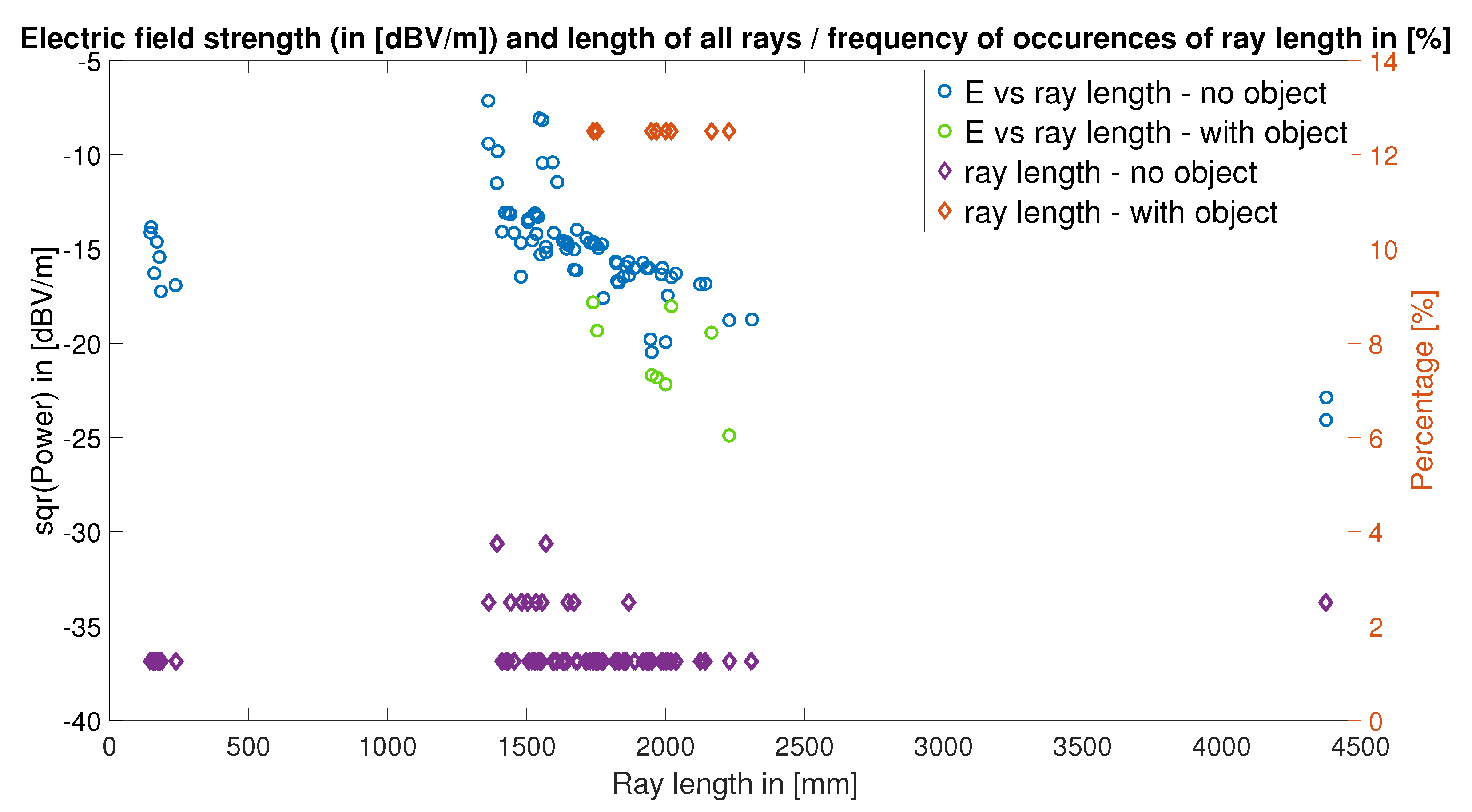
| Pos. 4—NO-LS | Antenova SR4W030 | 1.36/1.55/1.73/1.93/4.38 | −20.47/−16.35/−14.74/−13.11/−0.80 | 7.0% |
| Pos. 4—NO-LS | Laird 001-0015 | 1.37/1.52/1.71/1.90/2.21 | −27.44/−23.82/−22.33/−20.97/−12.45 | 3.2% |
| Pos. 4—O-LS | Antenova SR4W030 | 1.74/1.89/2.00/2.11/2.23 | −24.89/−21.33/−19.44/−18.04/−17.83 | 0.8% |
| Pos. 4—O-LS | Laird 001-0015 | n/a * | n/a * | 0.0% * |
| Pos. 3—NO-LS | Antenova SR4W030 | 1.30/1.55/1.89/2.36/4.42 | −18.03/−12.54/−9.47/−7.88/1.98 | 18.5% |
| Pos. 3—NO-LS | Laird 001-0015 | 1.29/1.56/1.94/2.24/4.21 | −17.32/−11.37/−8.35/−6.75/2.45 | 22.8% |
| ‘NO-LS’: No Object, Lid Shut | ‘O-LS’: With Object, Lid Shut | |||||||
|---|---|---|---|---|---|---|---|---|
| ID | Antenna | Rank | VNA-Based | EM-Simulation | Shift | VNA-Based | EM-Simulation | Shift |
| 1 | Antenova SR4W030 | 1 | 17 | 14 | −4 | 1 | 18 | −1 |
| 2 | Kyocera AVX1000418 | 2 | 20 | 1 | −1 | 17 | 1 | −1 |
| 3 | Kyocera AVX1001932PT | 3 | 1 | 20 | 1 | 11 | 17 | −3 |
| 4 | Laird 001-0015 | 4 | 2 | 18 | −3 | 20 | 20 | 0 |
| 5 | Laird 001-0034 ** | 5 | 18 | 17 | 1 | 21 | 21 | 0 |
| 6 | Laird CAF94505 | 6 | 3 | 21 | −3 | 18 | 11 | 5 |
| 7 | Laird MAF94264 *** | 7 | 21 | 2 | 1 | 4 | 2 | −1 |
| 8 | Molex 47950 * | 8 | 14 | 13 | 7 | 14 | 4 | −4 |
| 9 | Molex 146220 | 9 | 4 | 3 | −3 | 2 | 6 | 2 |
| 10 | Molex 204281 ** | 10 | 11 | 6 | −1 | 3 | 13 | −3 |
| 11 | Molex 206994 | 11 | 9 | 11 | −3 | 13 | 16 | 1 |
| 12 | Pulse Larsen W3334B0150 * | 12 | 6 | 4 | 2 | 6 | 14 | 3 |
| 13 | Taoglas FXP70070053A | 13 | 16 | 16 | 0 | 16 | 3 | 2 |
| 14 | Taoglas FXP74070100A | 14 | 13 | 9 | 6 | 9 | 9 | 0 |
| 15 | Taoglas FXP75070045B *** | 15 | 5 | 5 | 0 | 5 | 5 | 0 |
| 16 | Taoglas FXP810070100C | 16 | 7 | 7 | 0 | 7 | 7 | 0 |
| 17 | Taoglas WCM010151W | 17 | 8 | 8 | 0 | 8 | 8 | 0 |
| 18 | TE Connectivity 2118059 | 18 | 10 | 10 | 0 | 10 | 10 | 0 |
| 19 | Yageo ANTX100P001 *** | 19 | 12 | 12 | 0 | 12 | 12 | 0 |
| 20 | Yageo ANTX100P111 | 20 | 15 | 15 | 0 | 15 | 15 | 0 |
| 21 | Yageo ANTX100P113 | 21 | 19 | 19 | 0 | 19 | 19 | 0 |
Publisher’s Note: MDPI stays neutral with regard to jurisdictional claims in published maps and institutional affiliations. |
© 2022 by the authors. Licensee MDPI, Basel, Switzerland. This article is an open access article distributed under the terms and conditions of the Creative Commons Attribution (CC BY) license (https://creativecommons.org/licenses/by/4.0/).
Share and Cite
Kraus, D.; Diwold, K.; Pestana, J.; Priller, P.; Leitgeb, E. Towards a Recommender System for In-Vehicle Antenna Placement in Harsh Propagation Environments. Sensors 2022, 22, 6339. https://doi.org/10.3390/s22176339
Kraus D, Diwold K, Pestana J, Priller P, Leitgeb E. Towards a Recommender System for In-Vehicle Antenna Placement in Harsh Propagation Environments. Sensors. 2022; 22(17):6339. https://doi.org/10.3390/s22176339
Chicago/Turabian StyleKraus, Daniel, Konrad Diwold, Jesús Pestana, Peter Priller, and Erich Leitgeb. 2022. "Towards a Recommender System for In-Vehicle Antenna Placement in Harsh Propagation Environments" Sensors 22, no. 17: 6339. https://doi.org/10.3390/s22176339