Application of a Bayesian Network Based on Multi-Source Information Fusion in the Fault Diagnosis of a Radar Receiver

Abstract

A radar is an important part of an air defense and combat system. It is of great significance to military defense to improve the effectiveness of radar state monitoring and the accuracy of fault diagnosis during operation. However, the complexity of radar equipment’s structure and the uncertainty of the operating environment greatly increase the difficulty of fault diagnosis in real life situations. Therefore, a Bayesian network diagnosis method based on multi-source information fusion technology is proposed to solve the fault diagnosis problems caused by uncertain factors such as the high integration and complexity of the system during the process of fault diagnosis. Taking a fault of a radar receiver as an example, we study 2 typical fault phenomena and 21 fault points. After acquiring and processing multi-source information, establishing a Bayesian network model, determining conditional probability tables (CPTs), and finally outputting the diagnosis results. The results are convincing and consistent with reality, which verifies the effectiveness of this method for fault diagnosis in radar receivers. It realizes device-level fault diagnosis, which shortens the maintenance time for radars and improves the reliability and maintainability of radars. Our results have significance as a guide for judging the fault location of radars and predicting the vulnerable components of radars.

1. Introduction

With the continuous progress of modern science and technology, an endless variety of new weapons have changed modern combat [1]. In modern war, air attacks are often used as the main means of warfare. Now more than ever, gaining control of the air has become vitally important. Radars have thus become indispensable equipment in the air defense system of various countries.

A radar is an electronic device that can work all day and in all weather conditions [2]. Due to the demanding tasks and long operation time of radars, the equipment failure rate has increased markedly. A radar receiver is an important component of a radar system. It performs pre-selection, amplification, frequency conversion, filtering, demodulation, and digital processing on the echo signal received by the radar antenna while suppressing external interference clutter and internal noise so that the echo signal can maintain the target information as much as possible in order to conduct further specialized signal processing [3]. Once the radar receiver fails, the radar is not able to accurately detect the target, which affects the normal operation of the entire air defense system [4]. Therefore, it is of great significance to strengthen the condition monitoring of radar receivers, analyze and evaluate important parameters, diagnose faults in time, and quickly formulate solutions.

With the development of artificial intelligence technology and the improvement of signal processing accuracy, technologies such as wavelet transform [5,6], support vector machines [7,8], principal component analyses [9,10], artificial neural networks [11,12,13], and deep learning [14,15,16] have been widely used in the field of fault diagnosis. These methods are able to learn and mine historical data under certain functional constraints to discern the corresponding relationship of a data model and then approach the mapping mechanism implied in the system data to carry out fault detection and diagnosis [17]. Based on monitoring data from different sources and types, this method solves the problem of incomplete fault representation and has real-time capabilities. However, this method invariably depends on the accuracy of the mathematical model and the real-time nature of the data and is restricted by factors such as the number of data and the calculation efficiency of the model. In most cases, these models they are unable to explain their reasoning processes and results, and there are different degrees of defects in the treatment of uncertainty problems.

Bayesian networks, proposed by Judea pearl in 1988, have powerful uncertainty problem processing abilities and are widely used in computer intelligence science, industrial control, medical diagnosis, and other fields. Moreover, Bayesian network can effectively express and fuse multi-source information and have great advantages when identifying the faults caused by uncertainty and the correlation of complex equipment [18].

Traditional radar fault diagnosis is realized by built-in test equipment (BITE). BITE is distributed in each function module of the radar. It can detect faults in equipment components and identify the faulty components. The maintenance personnel can then replace the faulty parts to eliminate the fault. The diagnostic process of BITE is shown in Figure 1.

When using BITE technology for maintenance support, the average fault recovery time (MTBR) of a radar is less than 10 min, but this equipment comes with many shortcomings. BITE lacks the ability to detect and isolate intermittent faults. Moreover, due to the direct replacement of the faulty modules, the service life of the components is generally reduced, resulting in an increase of 10–20% in the manufacturing and maintenance cost of a radar [19]. How to accurately and quickly locate the fault point inside the component and build a circuit board-level or even device-level fault diagnosis system is an unsolved problem that is worthy of study.

However, due to the compact and complex structure of modern radars and the high internal integration of their components [20], if a bite circuit is embedded in the components, it will not only have great requirements in terms of space utilization but may also have a certain impact on the signals passing through the components. The echo signal reflected from the target received by a radar antenna is very weak, unstable, and cluttered [21]. The impact of bit circuit embedding on the echo signal cannot be ignored, which means that BITE embedded in the receiver component is not feasible.

In addition, there is no differentiation between fault phenomena and causes in the system operation. A fault often manifests itself in a variety of fault phenomena, and sometimes several faults will be reflected by only a single fault phenomenon. Therefore, the uncertainty between the fault phenomenon and the fault cause make fault diagnosis more complex [22].

In order to solve these problems, this paper proposes a Bayesian network fault diagnosis method based on multi-source information fusion technology. This method realizes intelligent fault detection and diagnosis in radar receiver and improves the service life of radar components. The contributions of this paper are summarized as follows:

• A variety of monitoring sensors are designed in the receiver. Based on multi-source information fusion technology, the prior diagnosis database and the real-time monitoring database reflected by the sensor are analyzed and fused to achieve the diversification, quantification, and standardization of the data.
• A Bayesian network fault diagnosis model is proposed and applied to the fault diagnosis analysis of a radar receiver. The analysis results show that this method is effective.
• In contrast to traditional BITE technology, our method can realize accurate device-level fault location and fault cause analysis and avoid the replacement of whole components, reducing the maintenance costs of radars.

The remainder of this paper is organized as follows. Section 2 introduces the fault diagnosis system of a radar receiver. Section 3 provides the sample data and calculation results. Section 4 presents an in-depth discussion of the calculation results. Finally, conclusions are drawn in Section 5.

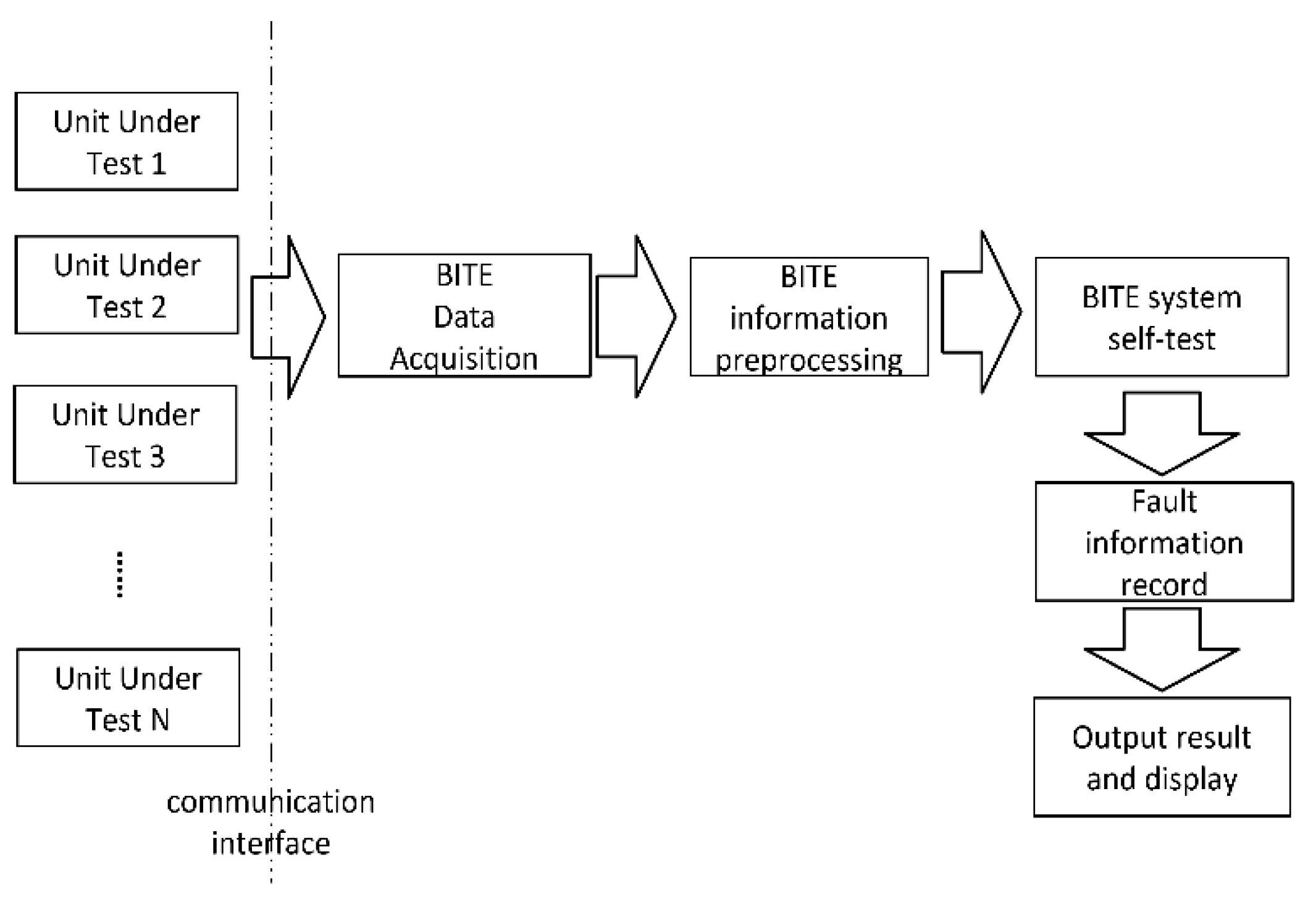
2. Fault Diagnosis System of Radar Receiver

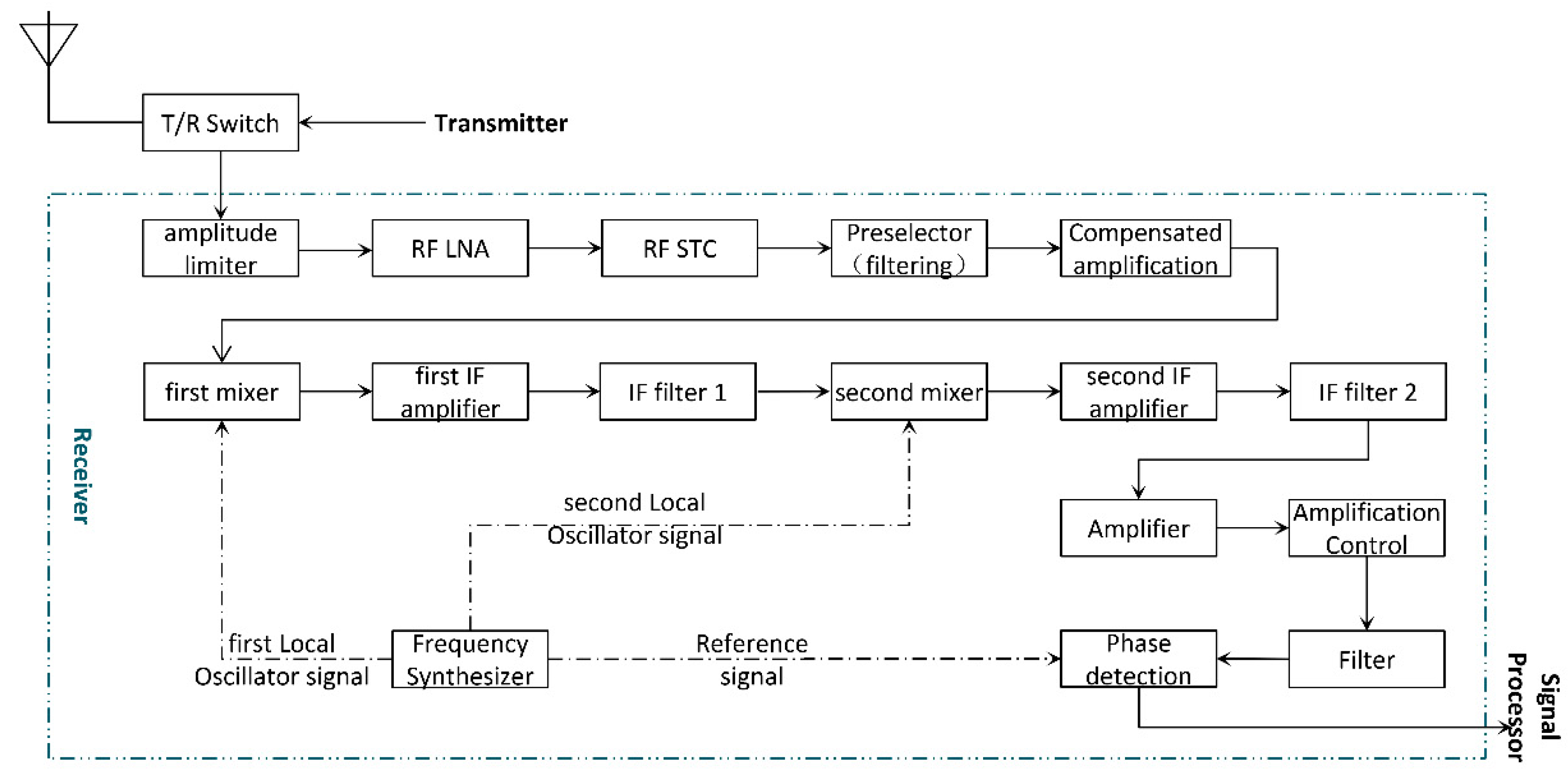
2.1. Radar Receiver

The input signal of the receiver is always very weak and needs to be amplified and filtered to meet professional signal processing requirements. Early radar receivers used multistage, high-frequency amplifiers to amplify the receive echo signals, which were called high-frequency amplification receivers [23]. Since then, superheterodyne receivers have become more widely used, which mainly rely on the fixed frequency intermediate frequency (IF) amplifier to amplify the signal. The basic structure of a superheterodyne receiver is shown in Figure 2.

A superheterodyne receiver is generally composed of a limiter, a radio frequency (RF) low noise amplifier (LNA), a sensitivity time control (STC) circuit, a RF filter, a mixer, an IF amplifier, an IF filter, a detection circuit, and a low-frequency power amplifier [24]. The echo signal received by the antenna enters the receiver through the transmitter/receiver (T/R) switch. The echo signal inherits the RF characteristics of the transmitted signal. The power of an echo signal is weak, but its frequency is high [25]. Therefore, the power of an echo signal needs to be amplified to meet the normal working power of the detector. However, the frequency of the echo signal needs to be down-converted into an IF signal. In practical radar receiver applications, especially when the working band is high and the bandwidth is wide, a secondary frequency conversion scheme is usually adopted. Once an IF signal that meets the requirements is obtained, the in-phase digital signal and quadrature digital signal are output through gain control and phase detection and sent to the digital signal processor [26]. The two local oscillator signals required for the mixer and the phase reference signal that are required for phase detection are generated by the frequency synthesizer.

2.2. Multi-Source Information Fusion Technology

The traditional fault diagnosis method only analyzes one or a small number of kinds of information from the machine state to extract information about the machine behavior. Practice has proven that although using one kind of information can sometimes identify faults in mechanical equipment, the diagnosis results obtained in many cases are not reliable. Due to the development of computers, signal processing, artificial intelligence, pattern recognition, and other technologies, a new fault diagnosis method based on multi-source information fusion technology has emerged [27].

Information fusion technology can be described as the automatic detection, association, estimation, and combination of multi-source data to obtain more accurate and reliable information or inferences. It is a global method of multi-dimensional data processing [28]. The fusion framework of multi-source information fusion technology is generally divided into three stages: data-level fusion, feature-level fusion, and decision-level fusion [29].

Data-level fusion is the direct fusion of the original data, which is mainly used for the fusion of data with relatively consistent information types, such as image analysis, signal processing, text data format conversion and so on. Data-level fusion maximizes the authenticity of the information, but its fault tolerance is weak. Additionally, the effect is not ideal for the fusion of information that includes many data types and complex relationships [30]. Feature-level fusion is used to conduct feature extraction from the information source and then to carry out association fusion on this basis. Feature-level fusion realizes the structural consistency of different types of information through feature extraction, retains ample information, provides support for later decision analysis, and improves real-time information processing ability, accuracy, and efficiency [31]. Decision-level fusion involves high-level fusion. Compared with data-level fusion and feature-level fusion, it has the greatest amount of information loss and the poorest accuracy, but it can process a wide range of data types with high flexibility, strong anti-interference ability, and good fault tolerance [32].

The multi-source information fusion fault diagnosis model used in our system is shown in Figure 3.

• Data Source

The data sources of the system are divided into prior diagnosis data sources and real-time data sources. The prior diagnosis data are mainly derived from expert experience, a case library, and historical monitoring data. The key points and conclusions of inspections, maintenance means, and maintenance steps summarized by professional maintenance technicians are used to compile the expert experience and case library, which are generally embodied in paper documents, electronic manuals, or oral experience inheritance. The historical detection data source is the operation data of the radar monitoring system or BITE since the radar has been operational. The BITE system of the radar is equipped with a single sensor, which is usually located inside the receiver in order to monitor the most important components in the receiver [33]. The operation data of the radar monitoring system or BITE only locate the fault at the level of the subsystem or the whole unit. The faults recorded in the expert experience and case library also have certain contingencies and cannot accurately reflect the current situation of the radar in real time [34]. If only a priori diagnosis data are used as the data source for the fault diagnostic model, it is unable to meet the requirements of fault diagnostic accuracy. Therefore, a variety of sensors are installed in the radar system to constantly monitor and inform the user of the status of the radar receiver.

An information processing method that uses multiple sensors to monitor the same specific target can overcome the uncertainty and limitations of a single sensor, obtain a consistent interpretation and description of the measured object, and realize the corresponding decision-making and estimation [35]. The type and number of sensors placed in the radar receiver can be determined according to the structure of the receiver and the parameter type of the monitored components.

Considering the complexity of the receiver’s high-frequency processing circuit and detection output circuit, as well as the variability of the environment, it can be added voltage sensors, current sensors, detection circuits, temperature sensors, humidity sensors, sound sensors, and cameras to monitor the voltage and current of the transmission path, the amplitude and phase of the signal, the sound of the internal action response in the components, and the temperature and humidity inside the receiver so as to achieve multi-directional and multi-dimension real-time monitoring and recording.

2.

Information Fusion

The original data collected from the data sources are diverse, so it is necessary to standardize the multi-source information before fusion.

It must carry out data standardization and format conversion on the a priori diagnostic data first, then convert them into a unified data format, and finally screen out useful information for correlation and calibration on the premise of consistent data types [36]. The data collected by various sensors may be waveforms, voltage values, current values, images, and so on. The data must be preprocessed to extract and identify the required information before fusion. Then the redundant, complementary, and conflicting information of the multiple sensors in the system is associated and calibrated by following certain rules. Finally, the information of the two data sources is fused to obtain a consistent description of the real situation of the measured object. This method provides more meaningful and valuable information for decision-making.

3.

Decision Discrimination

Effective information and decision theory are used to infer results [37]. Commonly used decision theories include the Kalman filter, the Dempster–Shafer evidence theory, expert knowledge systems, artificial neural networks, etc. Bayesian network reasoning is used in this paper. Bayesian networks have a strong ability to deal with uncertain problems. The construction of a Bayesian network consists of the determination of the network nodes, the directed correlation between the nodes, and the posterior probability. After reasoning through a Bayesian network, the final result of the fault diagnosis is output.

2.3. Bayesian Network

2.3.1. Brief Description

A Bayesian network is a directed graphic description based on a network structure that is the product of the integration of probability theory, graph theory, and decision theory [38].

It uses a structural directed graph to express the association relationship between the information elements and the influence node variables, uses the directed edge between nodes to connect the association relationship between elements, and uses conditional probability to express the influence degree of each information element.

Let $\mathrm{H}=\mathrm{X},\mathrm{L}$ denote a directed acyclic graph where $\mathrm{X}=\left\{X_1,X_2,\cdots ,X_n\right\}$ denotes the set of random variables and $\mathrm{L}$ denotes the set of edges of the Bayesian network, then the joint probability of $\mathrm{X}$ can be expressed as:

$$P\left(X_1,X_2,\cdots ,X_n\right)={{\displaystyle \prod }}_{i=1}^{n}P\left(X_i|Parents(X_i\right)=P\left(X_n|X_{n-1},\cdots ,X_1\right)P\left(X_2|X_1\right)P{X}_1$$

(1)

The basis of Bayesian network reasoning is the probability relationship between variables or events.

A Bayesian network can be regarded as the joint probability distribution of a group of random variables, from which reasoning and decision-making can be carried out [39]. All kinds of information related to fault diagnosis and maintenance decisions can be incorporated into a Bayesian network structure, which can handle it uniformly in the form of nodes and fuse different parts effectively according to the correlations between the information.

In addition, it can learn and reason under limited, incomplete, and uncertain information conditions and make reasonable and quantifiable decisions to maximize the decision efficiency [40].

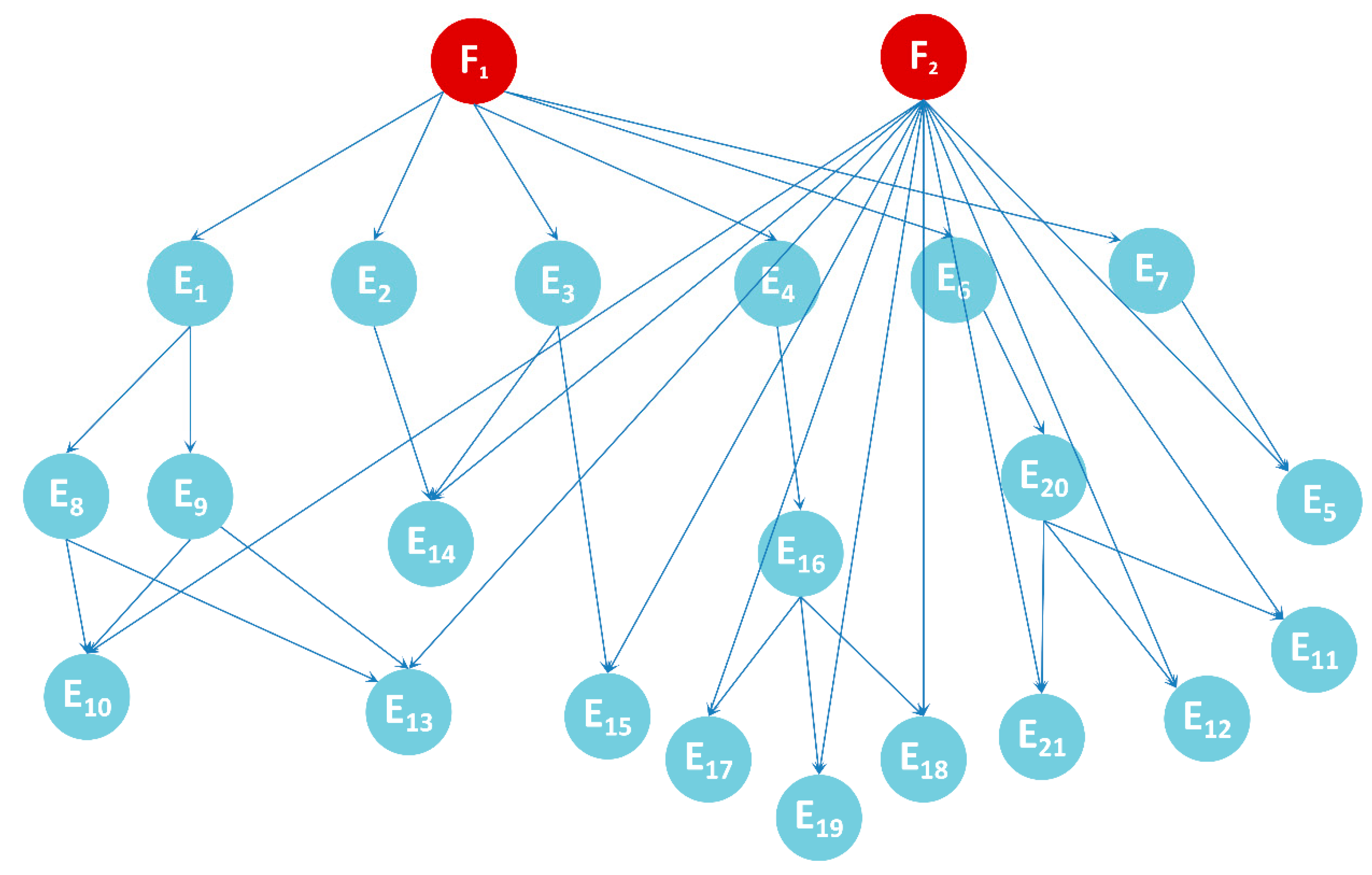
2.3.2. Determination of Bayesian Network

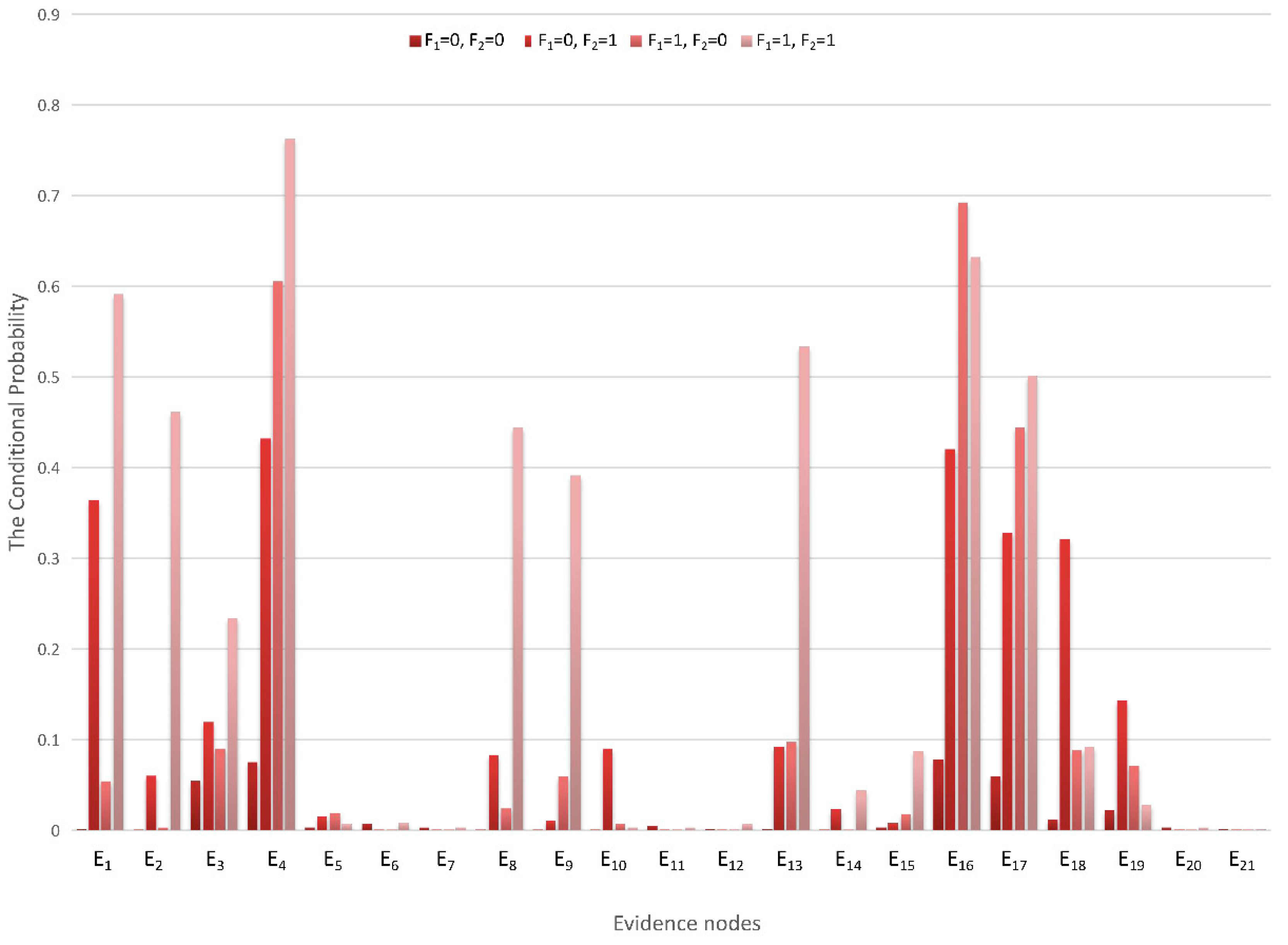
The main functions of the receiver are frequency conversion and phase detection [41]. There are many types of faults in these two functions. This paper takes the fault that the IF signal output obtained after the secondary mixing of the receiver is abnormal as an example to analyze the possible factors causing the fault.

Abnormal IF signal output indicates a variety of fault phenomena. The fault phenomena that may be detected include abnormal signal frequency, inconsistent multi-channel signal phase, inconsistent amplitude, low signal power, abnormal control voltage, high noise, high clutter, ineffective STC modulation, and so on. The corresponding fault points of these fault phenomena are shown in Figure 4.

The power supply is the energy source of the active devices in electronic circuits. The performance of the power supply directly affects the performance of electronic circuits. The power supply can be said to be the “heart” of electronic systems.

The frequency mixer, amplitude and phase corrector, amplitude limiter, frequency synthesizer, RF STC, power amplifier, and filter in the receiver all require electric energy, as well as a variety of power supplies with different voltages and capacities, to work normally.

The power converter is a special device in the radar receiver. It has two functions: voltage transformation and power supply. The external power supply enters the receiver, is transformed into the voltage values required by each component of the receiver through the power converter, and is then sent to each component to supply it with power. One power converter can convert the power supply to several voltage values, and the fault types of the power converter are also diverse. If a failure occurs in one voltage transformer branch of the power converter, the devices in the receiver that require a power supply from the transformer branch will not work. Once the power converter has a functional fault, there is no normal power supply for any of the electronic devices inside the receiver, meaning that the receiver will be in “paralysis”, as is shown in Figure 5.

By combining Figure 4 and Figure 5, the nodes and directed edges of the Bayesian network can be preliminarily determined so as to determine the Bayesian network model, as is shown in Figure 6.

F₁ and F₂ are two root nodes, which represent “abnormal IF signal output” and “power converter failure”, respectively. There are 21 causes that may lead to the F₁ phenomenon, which are represented by E₁–E₂₁. The F₂ phenomenon will make all components inoperative, resulting in the failure of the IF signal output and thus indirectly leading to the F₁ phenomenon. See

Table 1. Description of faults.

Nodes	Node Description	Monitoring Parameters
F1	Output IF signal is abnormal	Fault indicator of Receiver
F2	Power converter failure	Voltage

and

Table 2. Description of evidence nodes.

Nodes	Node Description	Monitoring Parameters
E1	Abnormal signal frequency	Frequency of Echo signal
E2	Inconsistent signal phase	Phase of signal Voltage
E3	Inconsistent signal amplitude	Amplitude of signal
E4	Low signal power	Power of signal
E5	RF STC failure	Amplitude of signal
E6	More clutter	Spectrum of signal
E7	Ineffective STC modulation	Amplitude of signal
E8	1st mixer inoperative	Frequency of signal
E9	2nd mixer inoperative	Frequency of signal
E10	Frequency synthesizer failure	No signal
E11	2nd IF filter failure	Spectrum of signal
E12	1st IF filter failure	Spectrum of signal
E13	Mixer failure	Voltage
E14	Amplitude and phase corrector failure	Amplitude and phase of signal
E15	Amplitude limiter failure	Amplitude of signal
E16	Power amplifier under power	Power of signal
E17	RF LNA failure	Power of signal
E18	2nd IF amplifier failure	Power of signal
E19	1st IF amplifier failure	Power of signal
E20	Insufficient filtering	Spectrum of signal
E21	Preselector failure	Spectrum of signal

for evidence definition and relevant information.

3. Results

Using the historical monitoring data of the radar, the conditional probability tables (CPTs) of all nodes can be determined in the fault diagnostic network. The prior probabilities of fault nodes F₁ and F₂ are shown in

Table 3. The prior probabilities of nodes F₁ and F₂.

Nodes	State (True/False)	P(Fx)
F1	1	P(F1) = 0.074
	0	P(F1) = 0.926
F2	1	P(F2) = 0.219
	0	P(F2) = 0.781

.

The parent node of the E₁, E₂, E₃, E₄, E₆, and E₇ events is F₁. The parent node of the E₅, E₁₀, E₁₁, E₁₂, E₁₃, E₁₄, E₁₅, E₁₇, E₁₈, E₁₉, and E₂₁ events is F₂. E₁ has the child nodes E₈, E₉, E₁₀, and E₁₃. If any of the child nodes fails, the fault phenomenon represented by E₁ is bound to occur.

The failure of E₁₀ and E₁₃ may be caused by F₂ power failure. Similarly, if E₁₇, E₁₈, or E₁₉ fails, E₁₆ and E₄ will occur, resulting in F₁ failure. By analogy, the posterior probabilities of other events are also extracted according to sample data processing and calculation. The results are shown in

Table 4. The conditional probabilities of evidence nodes E₁–E₂₁.

Nodes	F1	F2	E1	E2	E3	E4	E5	E6	E7
Probability	0	0	0.002	0.001	0.055	0.075	0.004	0.007	0.003
	0	1	0.364	0.060	0.120	0.432	0.015	0.001	0.001
	1	0	0.054	0.003	0.090	0.606	0.019	0.001	0.001
	1	1	0.592	0.462	0.234	0.763	0.007	0.008	0.004
Nodes	F1	F2	E8	E9	E10	E11	E12	E13	E14
Probability	0	0	0.001	0.001	0.001	0.005	0.002	0.002	0.001
	0	1	0.083	0.211	0.090	0.001	0.001	0.092	0.023
	1	0	0.024	0.059	0.007	0.001	0.001	0.098	0.001
	1	1	0.445	0.392	0.004	0.003	0.007	0.534	0.044
Nodes	F1	F2	E15	E16	E17	E18	E19	E20	E21
Probability	0	0	0.004	0.078	0.059	0.012	0.022	0.004	0.002
	0	1	0.009	0.421	0.328	0.322	0.143	0.001	0.001
	1	0	0.018	0.693	0.445	0.088	0.071	0.001	0.001
	1	1	0.087	0.632	0.501	0.092	0.028	0.003	0.002

.

With the calculations of the monitoring data samples and Bayesian network model, the CPTs can be denoted. Under different conditions of F₁ and F₂, the conditional probabilities of E₁–E₂₁ are different, and the posterior probabilities in the table can be transformed into a more intuitive chart form, as is shown in Figure 7.

4. Discussion

4.1. F₁ and F₂ Sub-Node Evidence

From the previous analysis, it can be seen that if the IF signal output is abnormal or the power converter fails, six fault phenomena will be directly caused; that is, the first layer child of nodes E₁, E₂, E₃, E₄, E₆, and E₇ events of F₁ and F₂. According to the CPTs, the relevant conditional probability distribution diagram can be obtained, which is shown in Figure 8.

In Figure 8, it can be seen that the event probability of node E₄ (low signal power) is the highest under any condition of F₁ and F₂.

Let $P_t$ be the power of the echo signal, $P_t$ be the power of the transmit signal, G be the receiving antenna gain, $\lambda$ be the transmitted electromagnetic wave length, $\sigma$ be the radar cross section, and R be the distance from the target to the radar. The Radar Equation can be obtained using the following equation:

$$P_r=\frac{P_t{G}^2\sigma {\lambda }^2}{{\left(4\pi \right)}^3{R}^4}$$

(2)

According to the radar equation, $P_r$ is inversely proportional to $R^4$. The farther the target that is detected, the weaker the power of the echo signal [42]. This is because the emitted electromagnetic wave will decay rapidly in the transmission process. The electromagnetic wave emitted by the radar is a radio frequency signal with great power, but the signal energy reflected by the target received by the radar is extremely weak and may be only 10⁻⁷–10⁻⁶ V. This signal can be received by the signal processor only after it is amplified to at least tens of volts. Therefore, whether the echo signal power can be amplified to a strength that the signal processor can recognize is one of the key methods of testing the performance of the receiver. The all-weather/all-day characteristics of the radar have higher requirements for the stability of the receiver power amplifier. The power gap between the echo signal received by the antenna and the IF signal transmitted to the signal processor is 10⁷–10⁸ orders of magnitude, which requires power amplifiers. Consequently, the failure of power amplifier efficiency to meet the requirements is the most likely cause of an unsatisfactory output signal from the receiver, which is consistent with the result of the maximum probability of node E₄ shown in Figure 8.

4.2. E₄ Sub-Node Evidence

The direct fault cause of E₄ (low signal power) evidence is E₁₆ (power amplifier under power). According to a previous circuit analysis, general superheterodyne receivers have the tertiary power amplifier RF LNA for the 1st IF amplifier and 2nd IF amplifier. If any of the three amplifiers fails, E₄ (low signal power) evidence will be observed. The power of the echo is weak, but it inherits the high frequency of the transmitted signal. The RF low-noise amplifier is the first station for echo signal amplification. It should not only be able to withstand high-frequency signals but also undertake power amplifier tasks, which are required to suppress the interference of noise to improve the signal-to-noise ratio. Compared with the 1st IF amplifier and 2nd IF amplifier, the RF LNA is the most vulnerable device in the receiver, and it has a higher probability of failure. E₄ has four sub-nodes, E₁₆–E₁₉, which correspond to power amplifier under power, RF LNA failure, 1st IF amplifier failure, and 2nd IF amplifier failure events, respectively. Their conditional probability distributions are shown in Figure 9.

In Figure 9, E₁₆ has the highest probability because it is the direct cause of the low power of the signal. E₁₇–E₁₉ are the child nodes of E_16. Among them, E₁₇ (RF LNA failure) has the highest probability, which is in line with the circuit analysis results.

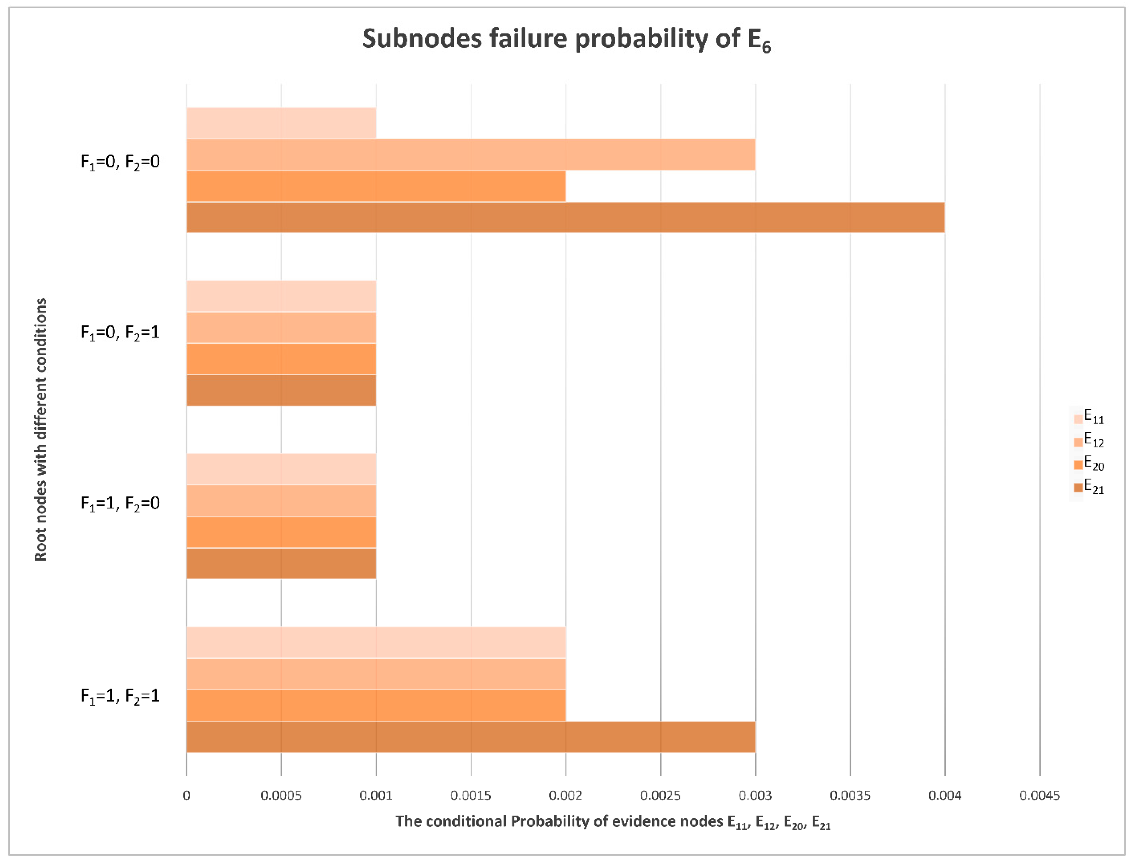
4.3. E₆ and E₇ Sub-Node Evidence

In addition to E₄ (low signal power), which is the most likely fault phenomenon, there may also be abnormal output frequency, inconsistent phase, inconsistent amplitude, abnormal control voltage, more clutter, ineffective STC modulation, etc. It can be seen from Figure 8 that, compared with other fault phenomena, the probabilities of E₆ (more clutter) and E₇ (ineffective STC modulation) are very low and can basically be ignored. It is indicated that the clutter suppression and STC control effect are the best and the possibility of failure is lowest in the receiver. The conditional probability distribution of an RF STC fault is shown in Figure 10, and the conditional probability distributions of the sub-nodes of E₆ (more clutter) are shown in Figure 11.

If the IF signal output is abnormal and the power converter has no faults, the probability of E₅ (RF STC failure) is the highest.

The direct cause of more clutter is E₂₀ (insufficient filtering) in the receiver. The filtering effect is basically subject to the three filters in the receiver. Under the same conditions, the failure probability of these three filters is almost the same, and because the probability of E₆ is very low, the failure probability of the filter can also be ignored.

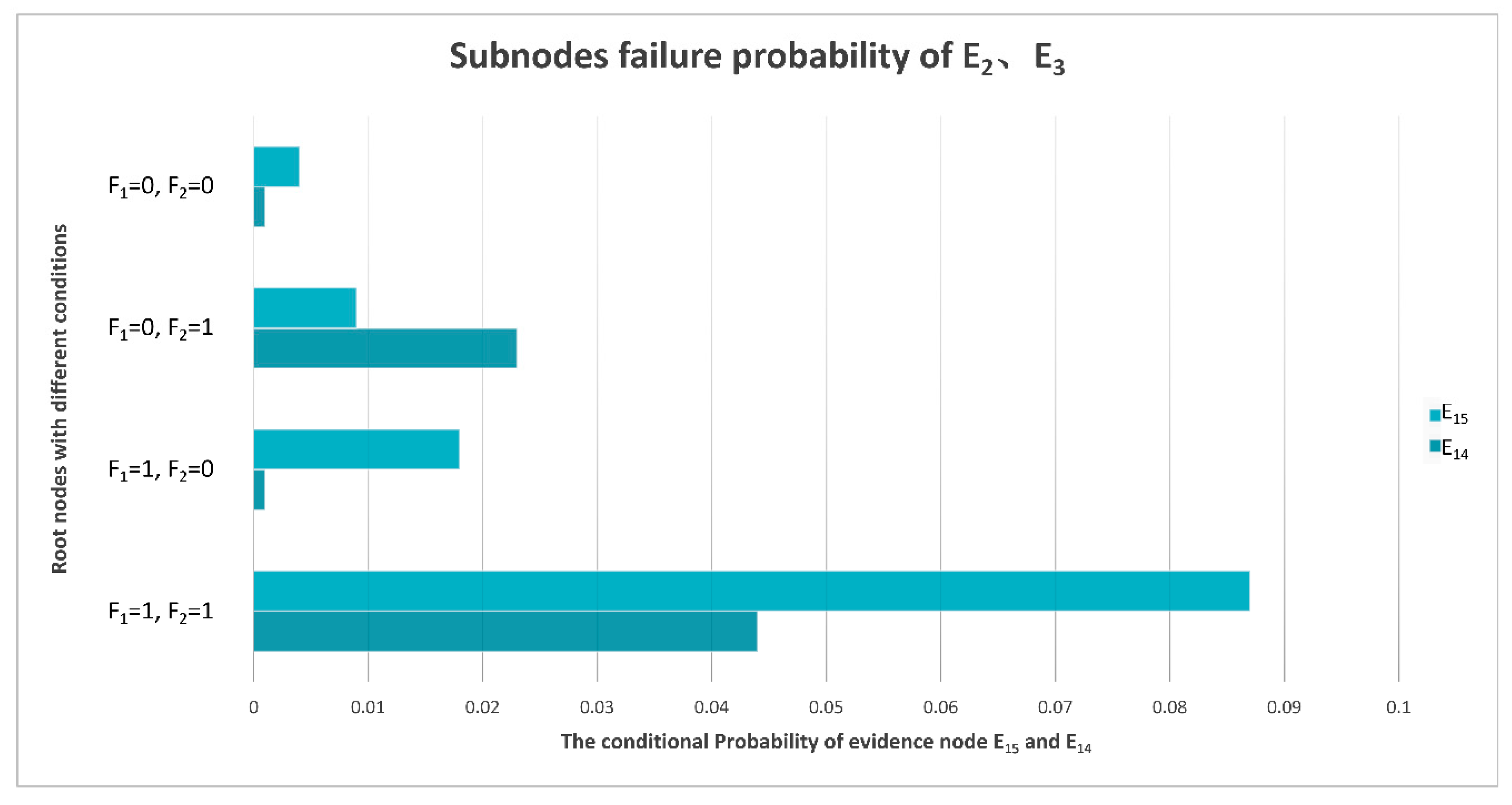
4.4. E₂ and E₃ Sub-Node Evidence

Generally speaking, the probability of an inconsistent phase or amplitude of the IF signal output by the receiver is not high. The probability of these two phenomena will increase only when the power converter fails, and the electronic components cannot work normally. The inconsistent phase and amplitude may be caused by the poor effect of the amplitude and phase corrector and amplitude limiter. The conditional probability distribution of E₂ and E₃ sub-nodes is shown in Figure 12.

In most cases, the probability of limiter failure is higher than that of other kinds of failures. When the power converter fails, the probability of amplitude and phase corrector failure increases.

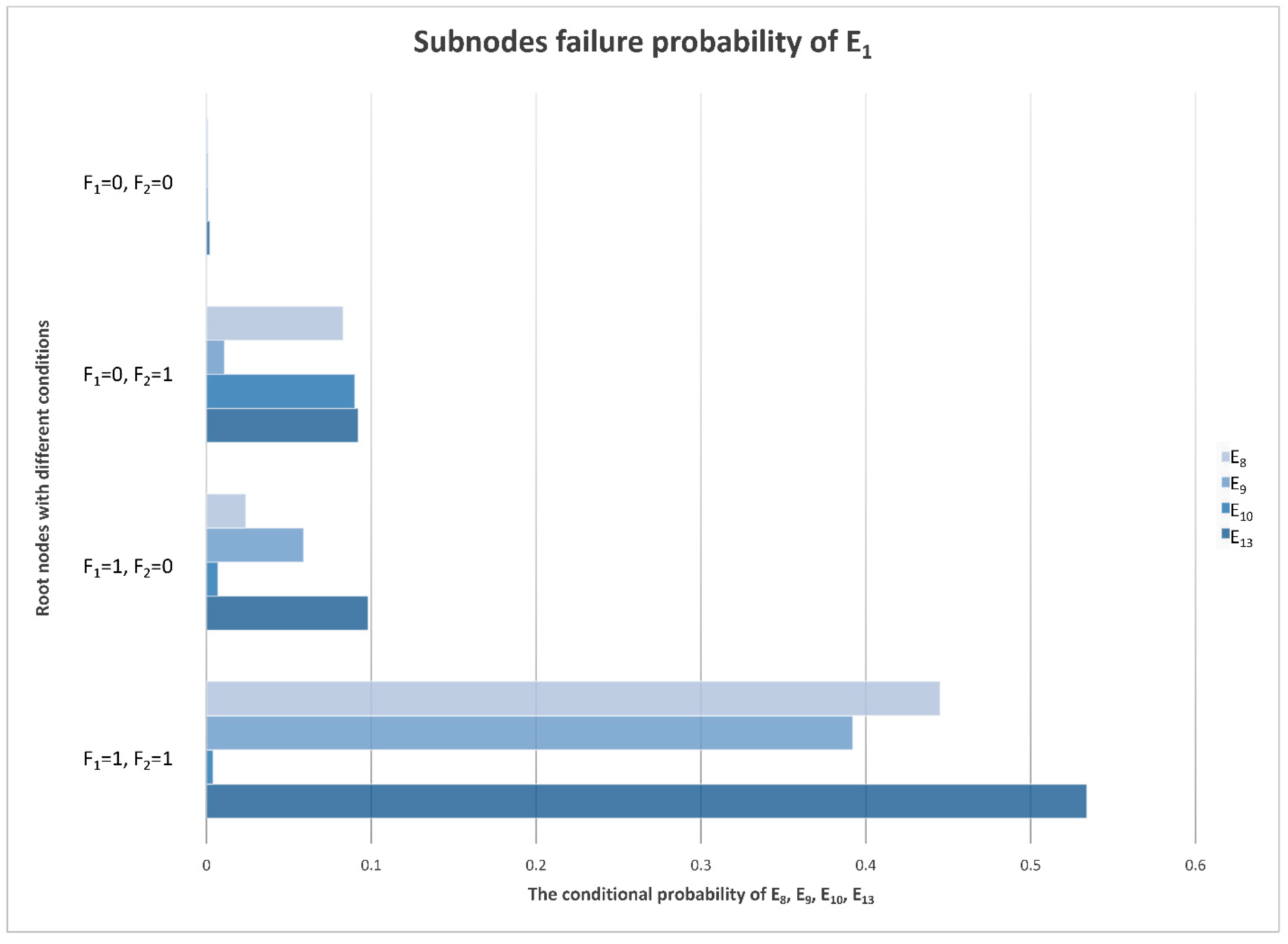
4.5. E₁ Sub-Node Evidence

In addition to amplifying the echo signal, the main task of the receiver is to reduce the frequency of the echo signal and convert the RF signal into an IF signal through down-conversion [43]. The abnormal frequency of the final IF output signal is uncommon. If the frequency is abnormal, it means that the mixing effect is not ideal; mixers and local oscillator signals are the factors that influence the mixing effect. The local oscillator signals come from the frequency synthesizer. The conditional probability distributions of the sub-nodes of E₁ (abnormal signal frequency) are shown in Figure 13.

In the mixing process of the receiver, if the local oscillator signals are abnormal, it will report a fault in the frequency synthesizer and will not enter the mixer without warning. Therefore, compared with the local oscillator signals, the failure probability of the mixer is higher. The mixer is also an electronic device and needs a power supply. In the case of a power converter failure, the failure probability of the mixer is higher.

5. Conclusions

This paper provides a Bayesian fault diagnosis method based on multi-source information fusion. This method determines the Bayesian network model by processing and fusing expert experience data, a case library, historical monitoring data, and data obtained from various sensors according to the relationship between fault phenomena and causes, as well as the circuit structure characteristics of the radar receiver. Then, by calculating the conditional probability of each node, the device that is most likely to cause the fault is output, which proves the effectiveness of this method. This fault diagnosis method optimizes the component level fault alarm (which is completed by BITE at the moment), locates the fault points at the device level, avoids the waste of resources caused by the replacement of a whole piece during radar maintenance, and improves the efficiency and cost ratio of the maintenance process. In the future, the method proposed in this paper will be applied to the status monitoring and fault diagnosis of radar subsystems, such as transmitters, antenna feeders, recording terminal, power supplies, and so on, and the stability and accuracy of this method will be further improved through data collection and analysis.

References

1. Liu, B. On the development of military radar and its role in modern war. Dual Use Technol. Prod. 2018, 190. [Google Scholar] [CrossRef]
2. Chen, L.; Shen, X.; Tian, Q. SAR technique and its application to geologic and seismic research. Earthquake 2003, 23, 29–35. [Google Scholar] [CrossRef]
3. Qiang, Q.; Deng, F. Research and Analysis of the Radar Receiver Noise Characteristic. Value Eng. 2012, 31, 187–188. [Google Scholar] [CrossRef]
4. Zhu, Z. Analysis of Different Radar Receivers. Mod. Radar 2010, 32, 84–86. [Google Scholar] [CrossRef]
5. Wang, P.; Lee, C.-M. Fault Diagnosis of a Helical Gearbox Based on an Adaptive Empirical Wavelet Transform in Combination with a Spectral Subtraction Method. Appl. Sci. 2019, 9, 1696. [Google Scholar] [CrossRef]
6. Jayakumar, K.; Thangavel, S. Industrial drive fault diagnosis through vibration analysis using wavelet transform. J. Vib. Control JVC 2017, 23, 2003–2013. [Google Scholar] [CrossRef]
7. Jha, R.K.; Swami, P.D. Fault diagnosis and severity analysis of rolling bearings using vibration image texture enhancement and multiclass support vector machines. Appl. Acoust. 2021, 182, 108243. [Google Scholar] [CrossRef]
8. Fan, Q.; Yu, F.; Xuan, M. Transformer fault diagnosis method based on improved whale optimization algorithm to optimize support vector machine. Energy Rep. 2021, 7, 856–866. [Google Scholar] [CrossRef]
9. Schmid, M.; Endisch, C. Online diagnosis of soft internal short circuits in series-connected battery packs using modified kernel principal component analysis. J. Energy Storage 2022, 53, 104815. [Google Scholar] [CrossRef]
10. Han, Y.; Liu, J.; Liu, F.; Geng, Z. An intelligent moving window sparse principal component analysis-based case based reasoning for fault diagnosis: Case of the drilling process. ISA Trans. 2021. [Google Scholar] [CrossRef]
11. Naganathan, G.S.; Senthilkumar, M.; Aiswariya, S.; Muthulakshmi, S.; Santhiya Riyasen, G.; Mamtha Priyadharshini, M. Internal fault diagnosis of power transformer using artificial neural network. Mater. Today Proc. 2021. [Google Scholar] [CrossRef]
12. Kumar, A.; Singh, A.P. Transistor level fault diagnosis in digital circuits using artificial neural network. Measurement 2016, 82, 384–390. [Google Scholar] [CrossRef]
13. Shao, M.; Zhu, X.; Cao, H.; Shen, H. An artificial neural network ensemble method for fault diagnosis of proton exchange membrane fuel cell system. Energy 2014, 67, 268–275. [Google Scholar] [CrossRef]
14. Elsisi, M.; Tran, M.; Mahmoud, K.; Mansour, D.A.; Lehtonen, M.; Darwish, M.M.F. Effective IoT-based deep learning platform for online fault diagnosis of power transformers against cyberattacks and data uncertainties. Measurement 2022, 190, 110686. [Google Scholar] [CrossRef]
15. Wang, Z.; Xia, H.; Zhang, J.; Annor-Nyarko, M.; Zhu, S.; Jiang, Y.; Yin, W. A deep transfer learning method for system-level fault diagnosis of nuclear power plants under different power levels. Ann. Nucl. Energy 2022, 166, 108771. [Google Scholar] [CrossRef]
16. Shahin, S.; Xiang, L.; Jay, L. Deep learning-based cross-sensor domain adaptation for fault diagnosis of electro-mechanical actuators. Int. J. Dyn. Control 2020, 8, 1054–1062. [Google Scholar] [CrossRef]
17. Wen, C.; Lv, F.; Bao, Z.; Liu, M. A Review of Data Driven-based Incipient Fault Diagnosis. Acta Autom. Sin. 2016, 42, 1285–1299. [Google Scholar] [CrossRef]
18. Ye, S. Analysis on BITE management technology of modern air traffic control radar. Manag. Obs. 2011, 6–7. [Google Scholar] [CrossRef]
19. Yuan, H. The Modern Design Method about the Radar Mechanical Structure. Electro-Mech. Eng. 2000, 8–10. [Google Scholar] [CrossRef]
20. Gabella, M. Variance of Fluctuating Radar Echoes from Thermal Noise and Randomly Distributed Scatterers. Atmosphere 2014, 5, 92–100. [Google Scholar] [CrossRef] [Green Version]
21. Lai, Y.; Li, X. Reasoning strategies in uncertain situations for fault diagnosis of complex device. J. Electron. Meas. Instrum. 2011, 25, 117–123. [Google Scholar] [CrossRef]
22. Zeng, J.; Teng, Z. Data processes method of single-sensor based on maximum entropy. J. Electron. Meas. Instrum. 2012, 26, 1096–1099. [Google Scholar] [CrossRef]
23. Qian, M.; Yang, G.; Zhang, Y.; Jiang, C. Design of multi-channel VHF superheterodyne receiver. Mod. Electron. Tech. 2019, 42, 1–4, 10. [Google Scholar] [CrossRef]
24. Tohidian, M.; Madadi, I.; Staszewski, R.B. A Fully Integrated Discrete-Time Superheterodyne Receiver. IEEE Trans. Very Large Scale Integr. (VLSI) Syst. 2017, 25, 635–647. [Google Scholar] [CrossRef]
25. Chen, X.; Zeng, X. Adaptive Processing of Phase Coded Waveform Echo. Radar Sci. Technol. 2012, 10, 99–102, 111. [Google Scholar] [CrossRef]
26. Dong, Q.; Zhang, P. Design of Digital Synthetic Aperture Radar Receiver. Chin. J. Electron Devices 2008, 31, 572–575. [Google Scholar] [CrossRef]
27. Chen, K.; Zhang, Z.; Long, J. Multisource Information Fusion: Key Issues, Research Progress and New Trends. Comput. Sci. 2013, 40, 6–13. [Google Scholar] [CrossRef]
28. Juan, G.-R.; Serrano, M.A.; Patricio, M.A.; Jesús, G.; Molina, J.M. Context-based scene recognition from visual data in smart homes: An Information Fusion approach. Pers. Ubiquitous Comput. 2011, 16, 835–857. [Google Scholar] [CrossRef]
29. Li, X.; Song, J.; Qu, B.; Tian, M.; Xu, C.; Song, X.; Cai, W. Fault diagnosis technology of hydraulic powered support based on multilevel data fusion technology. Coal Sci. Technol. 2016, 44, 154–159. [Google Scholar] [CrossRef]
30. He, G.; Huo, H.; Fang, T. Scene classification based on feature-level and decision-level fusion. J. Comput. Appl. 2016, 36, 1262–1266. [Google Scholar] [CrossRef]
31. Rachid, B. Robust human action recognition scheme based on high-level feature fusion. Multimed. Tools Appl. 2012, 69, 253–275. [Google Scholar] [CrossRef]
32. Begum, S.; Barua, S.; Ahmed, M.U. Physiological Sensor Signals Classification for Healthcare Using Sensor Data Fusion and Case-Based Reasoning. Sensors 2014, 14, 11770. [Google Scholar] [CrossRef] [PubMed]
33. Czwartacka, A.; Lukasik, W.; Cholewa, J.; Jakubovvski, M. A BITE subsystem for phased array transmit antenna control. In Proceedings of the 15th International Conference on Microwaves, Radar and Wireless Communications (MIKON-2004), Warsaw, Poland, 17–19 May 2004; pp. 915–918. [Google Scholar]
34. Qian, L.; Liu, R. Application of BP Network to Fault Diagnosis of Radar Frequency Source. J. Air Force Radar Acad. 2008, 22, 117–119, 124. [Google Scholar] [CrossRef]
35. Biao, W.; Kelei, F.; Wenzhong, Y.; Zhiyu, Z. Study on multiple targets tracking algorithm based on multiple sensors. Clust. Comput. 2018, 22, 13283–13291. [Google Scholar] [CrossRef]
36. Wang, B.; Zhang, Y.; Jia, J. Ship Perception Information Fusion of Electronic Chart and Radar Image Based on Deep Learning Theory. Mod. Radar 2021, 43, 44–50. [Google Scholar] [CrossRef]
37. Wang, Z.; Zhao, P. Applying Method of Multi-Source Information Fusion to Achieving Early Diagnosis of Aero-Engine Rotor Fault. J. Northwestern Polytech. Univ. 2009, 27, 326–329. [Google Scholar] [CrossRef]
38. Arjun, S.; Brian, S.; Jeremy, S.; Olivier, H.; Margaret, M. Bayesian additional evidence for decision making under small sample uncertainty. BMC Med. Res. Methodol. 2021, 21, 221. [Google Scholar] [CrossRef]
39. Medkour, M.; Khochmane, L.; Bouzaouit, A.; Bennis, O. Transformation of Fault Trees into Bayesian Networks Methodology for Fault Diagnosis. Mechanika 2017, 23, 891–899. [Google Scholar] [CrossRef]
40. Lijia, X.; Zhiliang, K. Study on Fault Diagnosis for Radar′s Transmitter Based on Bayesian Network. In Proceedings of the 2010 2nd International Conference on Information Science and Engineering, Hangzhou, China, 4–6 December 2010; pp. 1530–1533. [Google Scholar]
41. Diskus, C.G.; Stelzer, A.; Gamsjäger, C.; Fischer, A.; Lübke, K.; Kolmhofer, E. Six-Port Receiver and Frequency Measurement for Radar Applications at 35GHz. Subsurf. Sens. Technol. Appl. 2000, 1, 271–288. [Google Scholar] [CrossRef]
42. Hou, J. Discussion on Radar Equation. Mod. Def. Technol. 2020, 48, 1–4, 38. [Google Scholar]
43. Gustafsson, A.; Alfredsson, M.; Danestig, M.; Malmqvist, R.; Ouacha, A. A fully integrated radar receiver front end including an active tunable band pass filter and an image rejection mixer. In Proceedings of the Microwave Conference, 2000 Asia-Pacific, Sydney, NSW, Australia, 3–6 December 2000; pp. 99–102. [Google Scholar]
Figure 1. BITE diagnosis flow chat.
Sensors 22 06396 g001
Figure 2. Structure Diagram of a Superheterodyne Receiver.
Sensors 22 06396 g002
Figure 3. The multi-source information fusion fault diagnosis model.
Sensors 22 06396 g003
Figure 4. Relationship between abnormal IF signal fault phenomenon and fault points.
Sensors 22 06396 g004
Figure 5. Relationship diagram of power converter fault.
Sensors 22 06396 g005
Figure 6. Bayesian network model.
Sensors 22 06396 g006
Figure 7. Conditional probability distribution diagram.
Sensors 22 06396 g007
Figure 8. Conditional probability distribution diagram of the first layer sub-nodes.
Sensors 22 06396 g008
Figure 9. Conditional probability distribution diagram of E4’s sub-nodes.
Sensors 22 06396 g009
Figure 10. Conditional probability distribution diagram of E5’s sub-nodes.
Sensors 22 06396 g010
Figure 11. Conditional probability distribution diagram of E6’s sub-nodes.
Sensors 22 06396 g011
Figure 12. Conditional probability distribution diagram of sub-nodes of E2 and E3.
Sensors 22 06396 g012
Figure 13. Conditional probability distribution diagram of E1’s sub-nodes.
Sensors 22 06396 g013