
Machine Learning-Based Prediction of Specific Energy Consumption for Cut-Off Grinding

 , ,
, ,  ,
,
Abstract
:1. Introduction
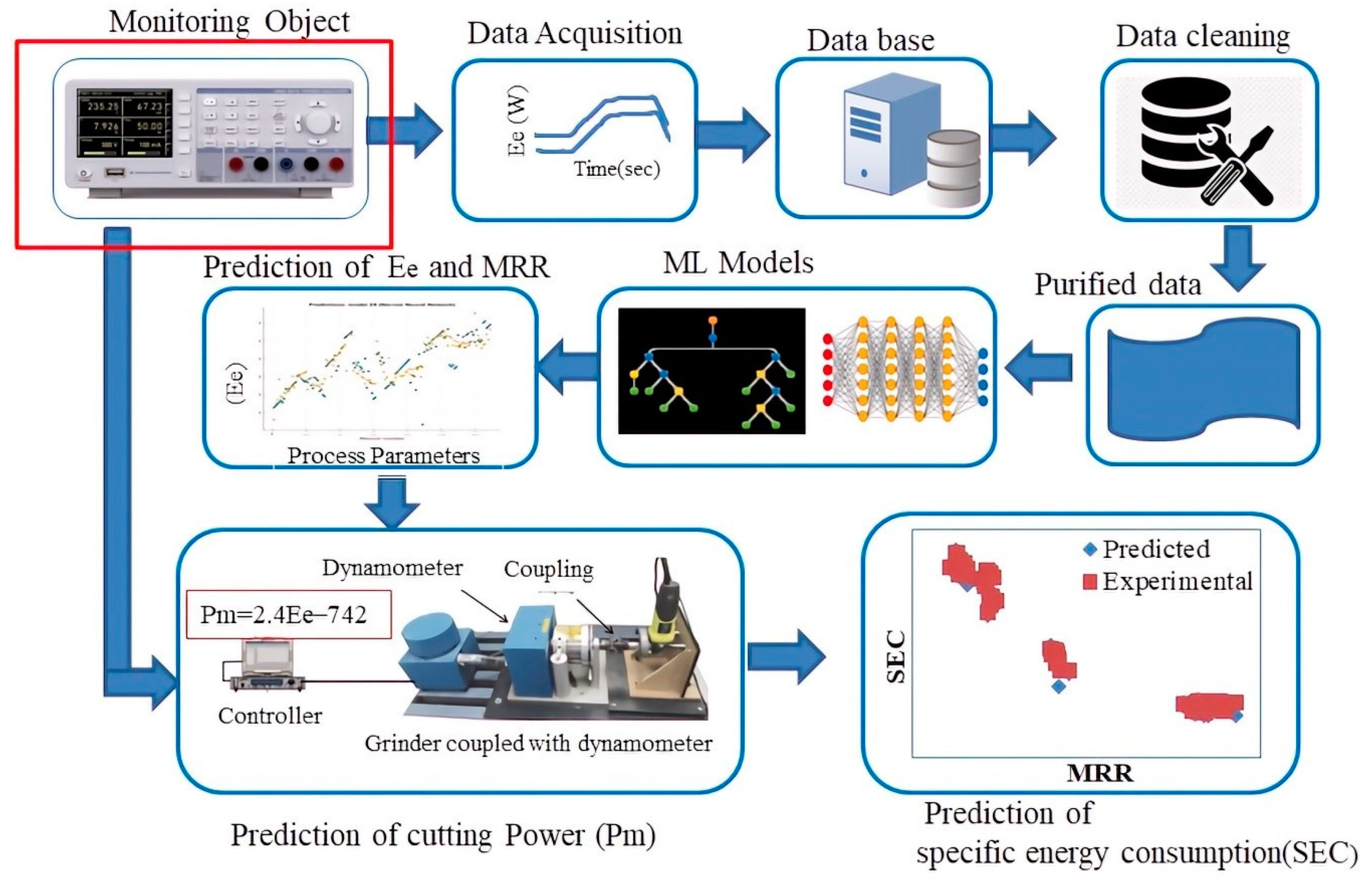
2. Methodology
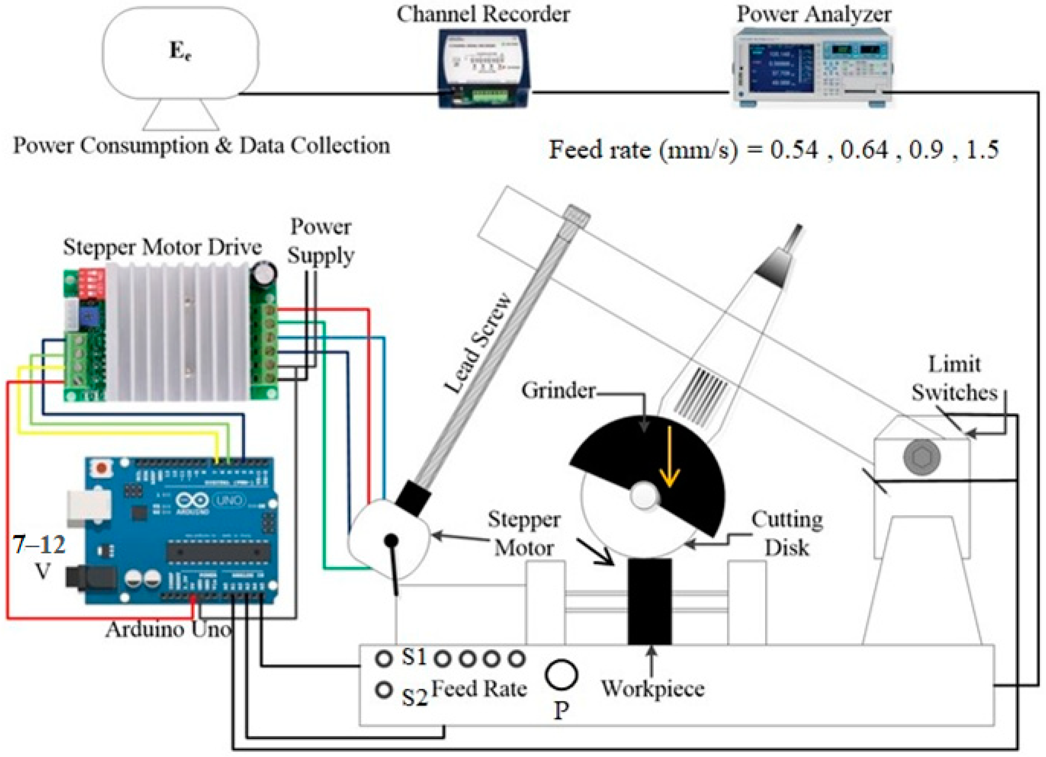
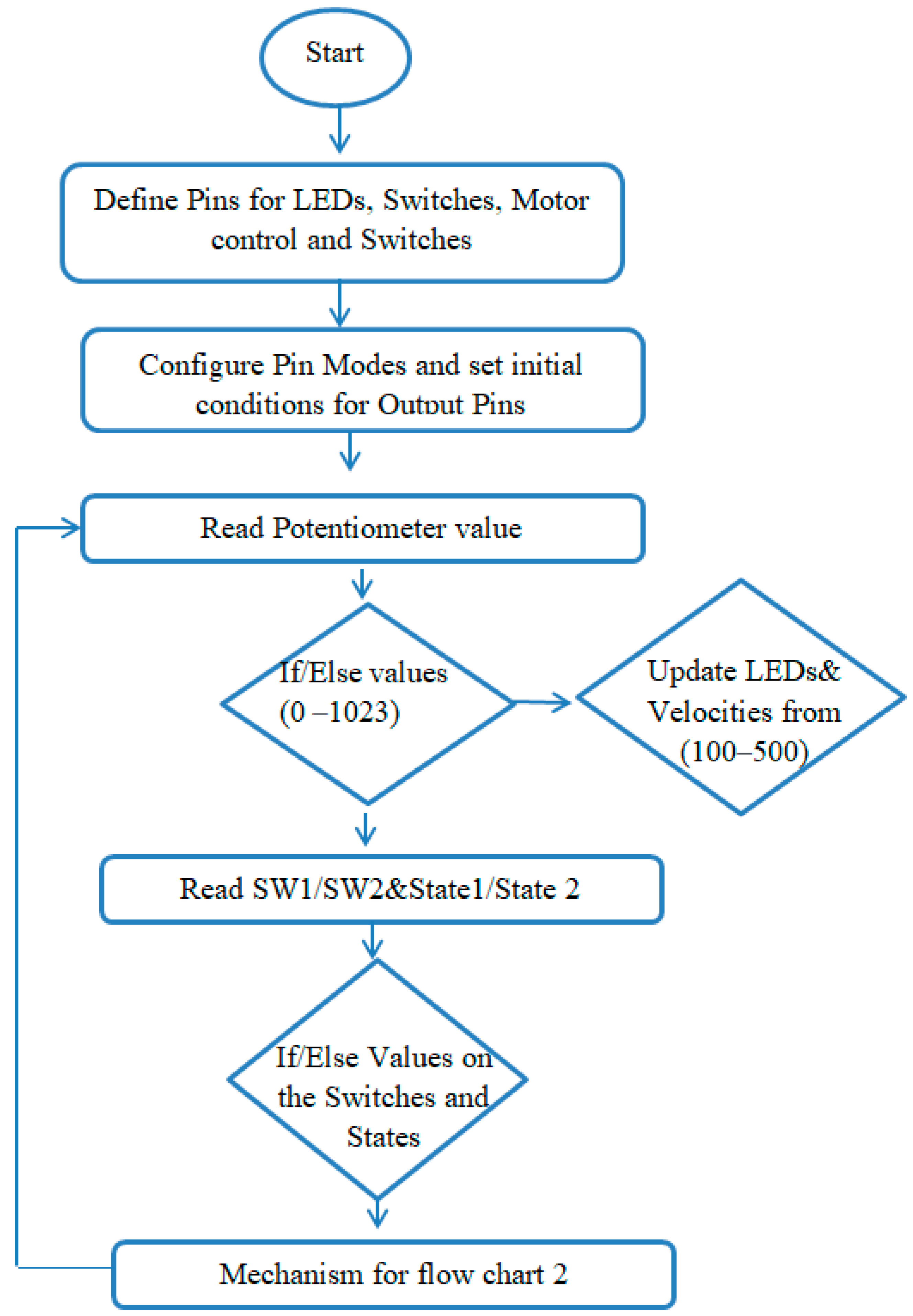
2.1. Design of Machine and Experimental Settings
2.2. Cutting Conditions
2.3. Data Acquisition
2.4. Data Processing and Machine Learning Models
2.4.1. Regression Trees
2.4.2. Gaussian Process Regression
2.4.3. Artificial Neural network
2.4.4. Performance Metrics
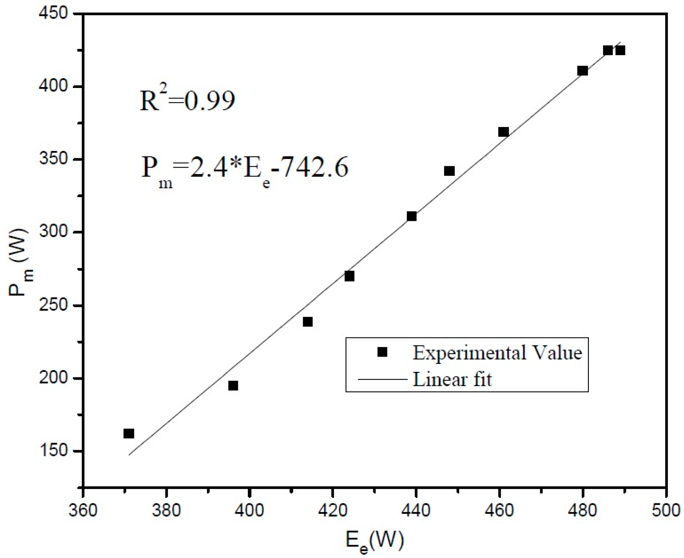
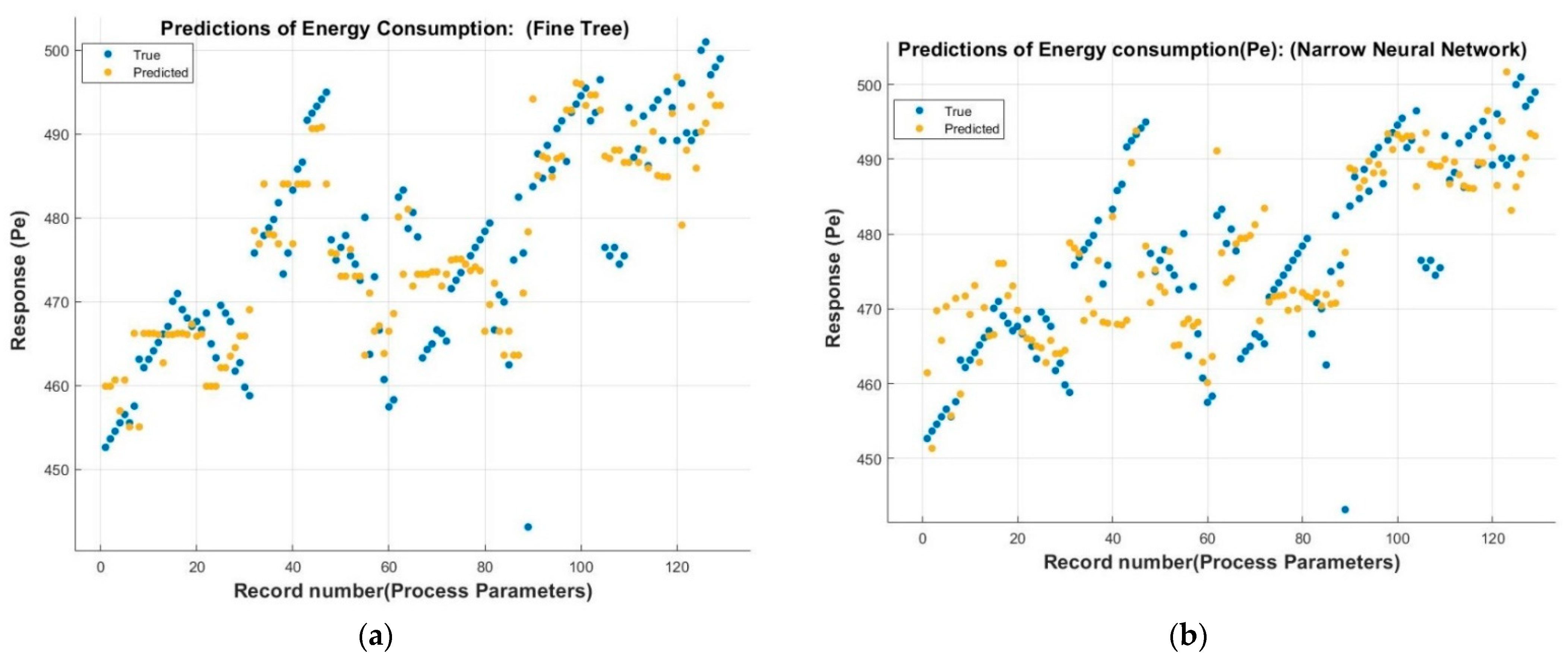
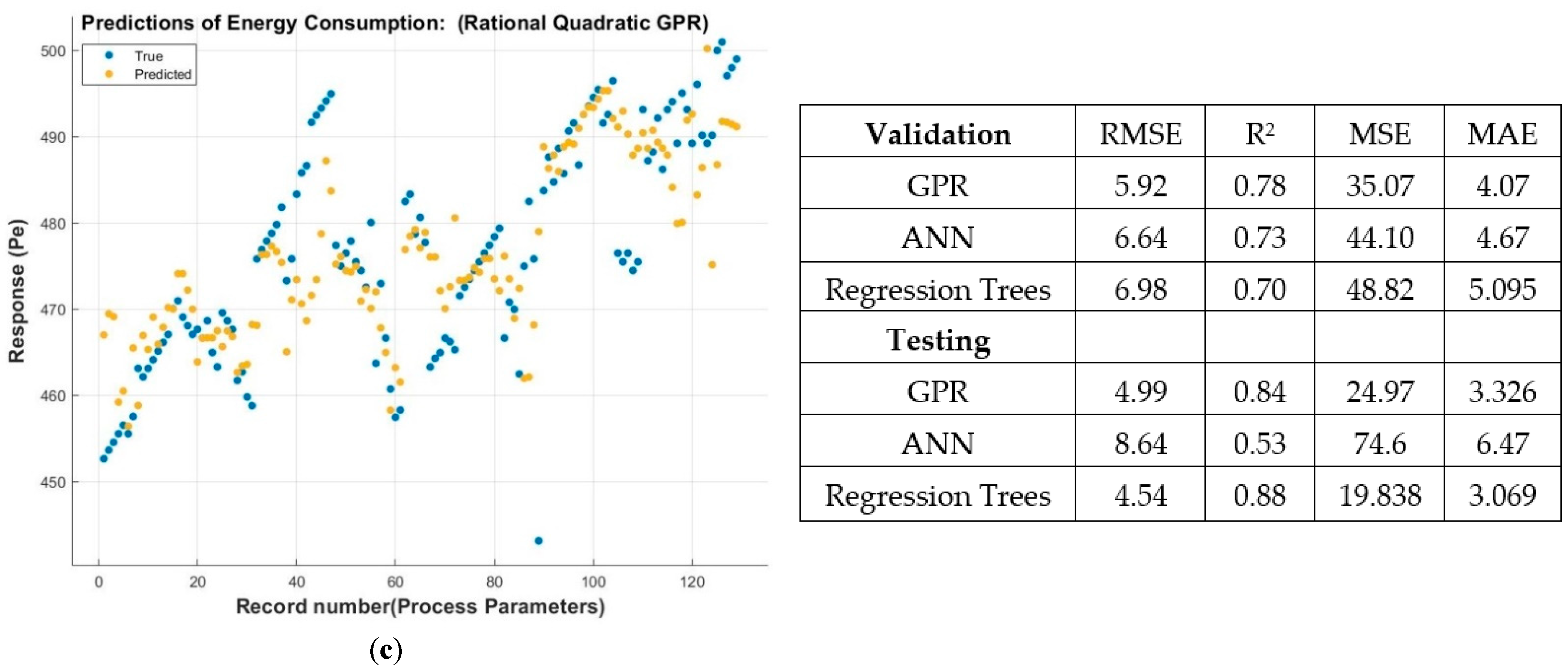
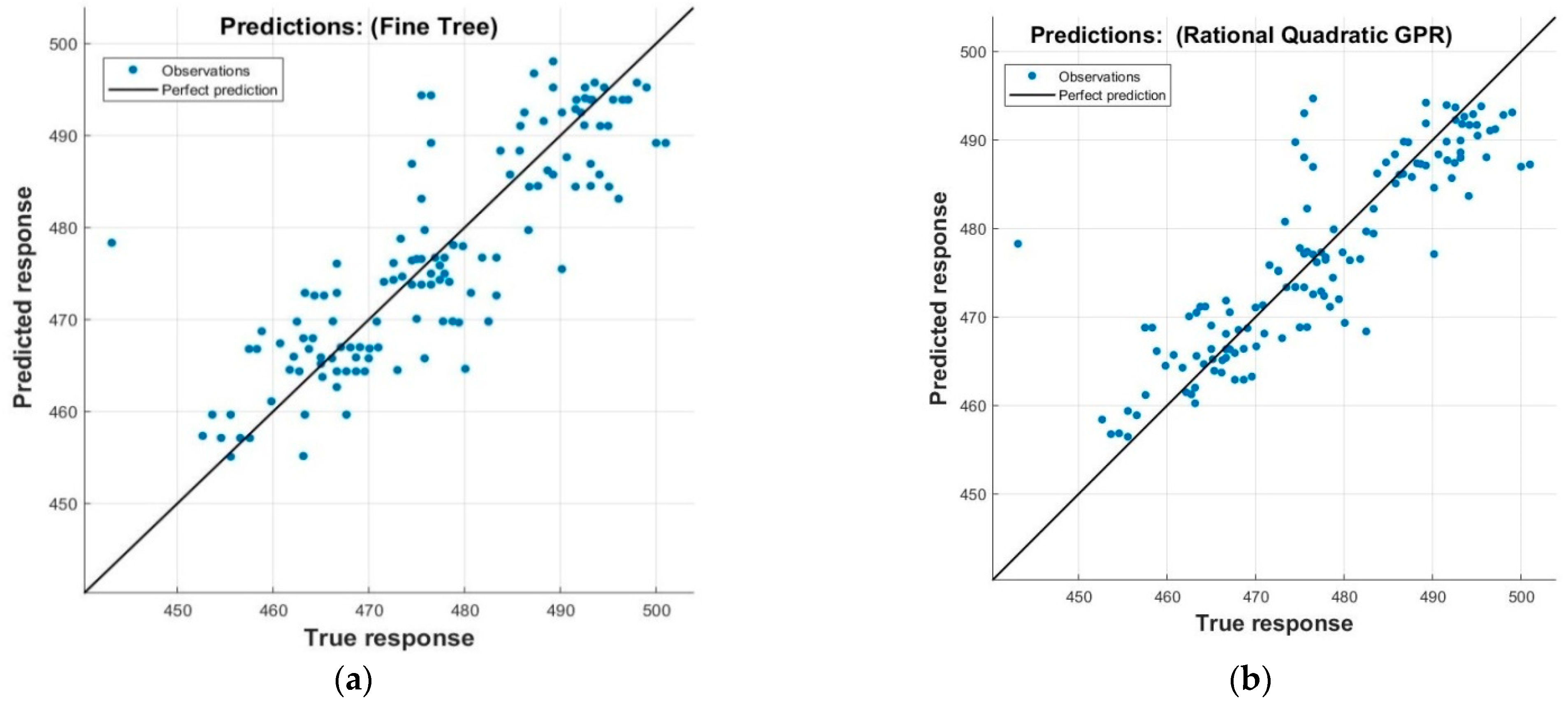
3. Results and Discussion
4. Conclusions
Author Contributions
Funding
Institutional Review Board Statement
Informed Consent Statement
Data Availability Statement
Conflicts of Interest
Appendix A

| Cutting Tool | Cutting Thickness (a) | Material Thickness (b) | Ac = a×b | Feed Rate (Vf) | MRR (Vf×a×b) | Pe (J) (Exp) | SEC (Exp) | SEC (Regression Trees) | SEC (ANN) | SEC (GPR) |
|---|---|---|---|---|---|---|---|---|---|---|
| 1.0 | 1.3 | 10.4 | 13.3 | 0.5 | 7.2 | 597 | 48.0 | 47.4 | 65.0 | 46.9 |
| 1.0 | 1.3 | 10.4 | 13.9 | 0.5 | 7.5 | 623 | 46.3 | 47.4 | 62.4 | 46.5 |
| 1.0 | 1.4 | 10.4 | 14.2 | 0.5 | 7.6 | 636 | 46.0 | 46.0 | 61.3 | 46.7 |
| 1.0 | 1.4 | 10.4 | 14.3 | 0.5 | 7.7 | 642 | 46.1 | 46.0 | 60.7 | 47.1 |
| 1.0 | 1.4 | 10.4 | 14.6 | 0.5 | 7.8 | 653 | 47.4 | 47.7 | 59.8 | 47.6 |
| 1.0 | 1.4 | 10.4 | 14.8 | 0.5 | 7.9 | 662 | 48.5 | 48.3 | 59.0 | 47.7 |
| 1.0 | 1.4 | 10.4 | 15.0 | 0.5 | 8.0 | 670 | 47.6 | 47.2 | 58.1 | 47.5 |
| 1.0 | 1.5 | 10.4 | 15.2 | 0.5 | 8.2 | 679 | 46.4 | 47.2 | 57.0 | 47.0 |
| 2.0 | 1.3 | 10.4 | 13.8 | 0.5 | 7.4 | 620 | 51.0 | 50.5 | 62.9 | 50.5 |
| 2.0 | 1.4 | 10.4 | 14.4 | 0.5 | 7.7 | 645 | 49.7 | 48.3 | 60.0 | 48.5 |
| 2.0 | 1.4 | 10.4 | 14.5 | 0.5 | 7.8 | 649 | 49.1 | 47.5 | 59.5 | 48.0 |
| 2.0 | 1.4 | 10.4 | 14.7 | 0.5 | 7.9 | 658 | 45.7 | 46.9 | 58.5 | 46.8 |
| 2.0 | 1.5 | 10.4 | 15.1 | 0.5 | 8.1 | 679 | 44.0 | 45.9 | 56.7 | 44.5 |
| 1.0 | 1.3 | 10.4 | 13.9 | 0.6 | 8.9 | 740 | 45.0 | 45.3 | 52.8 | 45.1 |
| 1.0 | 1.4 | 10.4 | 14.2 | 0.6 | 9.1 | 755 | 43.4 | 45.3 | 51.9 | 45.0 |
| 1.0 | 1.4 | 10.4 | 14.5 | 0.6 | 9.3 | 771 | 45.8 | 47.1 | 51.1 | 45.4 |
| 1.0 | 1.4 | 10.4 | 14.8 | 0.6 | 9.4 | 786 | 46.6 | 46.4 | 50.0 | 45.9 |
| 1.0 | 1.4 | 10.4 | 15.0 | 0.6 | 9.6 | 799 | 46.1 | 45.6 | 49.3 | 45.8 |
| 1.0 | 1.4 | 10.4 | 15.0 | 0.6 | 9.6 | 801 | 46.1 | 45.6 | 49.0 | 45.7 |
| 2.0 | 1.5 | 10.4 | 15.3 | 0.6 | 9.8 | 817 | 40.9 | 40.9 | 48.0 | 41.0 |
| 2.0 | 1.4 | 10.4 | 14.9 | 0.6 | 9.5 | 795 | 41.1 | 40.7 | 49.0 | 41.0 |
| 2.0 | 1.4 | 10.4 | 14.8 | 0.6 | 9.4 | 786 | 41.6 | 40.3 | 49.5 | 40.4 |
| 2.0 | 1.4 | 10.4 | 14.6 | 0.6 | 9.3 | 776 | 39.0 | 38.7 | 50.2 | 39.7 |
| 1.0 | 1.4 | 10.4 | 14.4 | 0.9 | 12.9 | 1075 | 32.2 | 31.6 | 36.9 | 32.2 |
| 1.0 | 1.4 | 10.4 | 14.5 | 0.9 | 13.0 | 1083 | 32.1 | 31.6 | 36.7 | 31.7 |
| 1.0 | 1.4 | 10.4 | 14.8 | 0.9 | 13.3 | 1106 | 30.4 | 30.8 | 36.1 | 29.8 |
| 1.0 | 1.4 | 10.4 | 15.0 | 0.9 | 13.4 | 1120 | 27.5 | 27.4 | 35.7 | 28.6 |
| 1.0 | 1.4 | 10.4 | 15.0 | 0.9 | 13.5 | 1127 | 27.6 | 27.4 | 35.5 | 28.1 |
| 1.0 | 1.5 | 10.4 | 15.3 | 0.9 | 13.8 | 1149 | 27.3 | 27.4 | 34.8 | 27.2 |
| 2.0 | 1.4 | 10.4 | 14.4 | 0.9 | 12.9 | 1077 | 30.1 | 30.5 | 36.8 | 30.7 |
| 2.0 | 1.4 | 10.4 | 14.4 | 0.9 | 12.9 | 1079 | 30.2 | 30.5 | 36.7 | 30.6 |
| 2.0 | 1.4 | 10.4 | 14.6 | 0.9 | 13.1 | 1091 | 30.8 | 30.5 | 36.4 | 30.0 |
| 2.0 | 1.4 | 10.4 | 14.8 | 0.9 | 13.3 | 1109 | 29.8 | 29.2 | 35.9 | 29.0 |
| 2.0 | 1.4 | 10.4 | 14.9 | 0.9 | 13.4 | 1113 | 31.1 | 29.2 | 35.8 | 28.7 |
| 1.0 | 1.4 | 10.4 | 14.5 | 1.5 | 21.5 | 1795 | 19.4 | 20.0 | 22.7 | 19.7 |
| 1.0 | 1.4 | 10.4 | 14.7 | 1.5 | 21.8 | 1818 | 19.4 | 19.0 | 22.5 | 19.6 |
| 1.0 | 1.4 | 10.4 | 14.9 | 1.5 | 22.1 | 1843 | 19.8 | 19.5 | 22.3 | 19.6 |
| 1.0 | 1.5 | 10.4 | 15.1 | 1.5 | 22.5 | 1878 | 19.5 | 19.7 | 21.9 | 19.5 |
| 1.0 | 1.5 | 10.4 | 15.2 | 1.5 | 22.7 | 1889 | 19.7 | 19.7 | 21.7 | 19.5 |
| 1.0 | 1.5 | 10.4 | 15.3 | 1.5 | 22.8 | 1902 | 19.2 | 19.4 | 21.6 | 19.4 |
| 2.0 | 1.4 | 10.4 | 14.8 | 1.5 | 22.0 | 1830 | 18.3 | 19.5 | 22.2 | 19.8 |
| 2.0 | 1.4 | 10.4 | 14.6 | 1.5 | 21.7 | 1807 | 18.4 | 19.3 | 22.5 | 19.9 |
| 2.0 | 1.4 | 10.4 | 14.3 | 1.5 | 21.3 | 1773 | 18.8 | 19.2 | 22.9 | 20.1 |
| 2.0 | 1.4 | 10.4 | 14.3 | 1.5 | 21.3 | 1777 | 20.0 | 20.9 | 22.8 | 20.1 |
| 2.0 | 1.4 | 10.4 | 14.1 | 1.5 | 21.0 | 1749 | 20.5 | 20.5 | 23.2 | 20.4 |
| 2.0 | 1.4 | 10.4 | 14.7 | 1.5 | 21.9 | 1821 | 20.4 | 20.2 | 22.3 | 19.8 |
| 2.0 | 1.5 | 10.4 | 15.7 | 1.5 | 23.4 | 1947 | 18.9 | 21.0 | 21.1 | 18.8 |
| 2.0 | 1.4 | 10.4 | 14.1 | 1.5 | 21.0 | 1754 | 21.3 | 20.8 | 23.1 | 20.3 |
| 2.0 | 1.3 | 10.4 | 13.8 | 1.5 | 20.6 | 1715 | 21.1 | 20.8 | 23.6 | 20.9 |
| 2.0 | 1.4 | 10.4 | 14.5 | 1.5 | 21.5 | 1792 | 20.1 | 21.2 | 22.6 | 19.9 |
| 2.0 | 1.4 | 10.4 | 15.0 | 1.5 | 22.3 | 1857 | 20.2 | 21.4 | 21.9 | 19.8 |
| 2.0 | 1.5 | 10.4 | 15.2 | 1.5 | 22.6 | 1883 | 20.1 | 21.4 | 21.6 | 19.7 |
References
- Papetti, A.; Menghi, R.; Di Domizio, G.; Germani, M.; Marconi, M. Resources value mapping: A method to assess the resource efficiency of manufacturing systems. Appl. Energy 2019, 249, 326–342. [Google Scholar] [CrossRef]
- Rahimifard, S.; Seow, Y.; Childs, T. Minimising Embodied Product Energy to support energy efficient manufacturing. CIRP Ann.-Manuf. Technol. 2010, 59, 25–28. [Google Scholar] [CrossRef]
- Rowe, W.B. Principles of Modern Grinding Technology; Elsevier: Amsterdam, The Netherlands, 2013. [Google Scholar]
- Yingjie, Z. Energy efficiency techniques in machining process: A review. Int. J. Adv. Manuf. Technol. 2014, 71, 1123–1132. [Google Scholar] [CrossRef]
- Awan, M.R.; Rojas, H.A.G.; Benavides, J.I.P.; Hameed, S. Experimental technique to analyze the influence of cutting conditions on specific energy consumption during abrasive metal cutting with thin discs. Adv. Manuf. 2021, 10, 260–271. [Google Scholar] [CrossRef]
- Komanduri, R.; Iyengar, S. Conventional and Super Abrasive Materials. In Encyclopedia of Materials: Science and Technology; Elsevier: Amsterdam, The Netherlands, 2001; pp. 1629–1651. [Google Scholar]
- Nelson, J.A.; Westrich, R.M. Abrasive Cutting in Metallography. In Metallographic Specimen Preparation; Springer: New York, NY, USA, 1974; pp. 41–54. [Google Scholar]
- Hahn, R.S. On the Nature of the Grinding Process. Available online: https://scholar.google.com/scholar?hl=en&as_sdt= (accessed on 26 March 2021).
- Singh, V.; Rao, P.V.; Ghosh, S. Development of specific grinding energy model. Int. J. Mach. Tools Manuf. 2012, 60, 1–13. [Google Scholar] [CrossRef]
- Sinha, M.K.; Paruchuri, V.R.; Kumar, P.; Ghosh, S.; Venkateswara Rao, P. An Improved Model for Specific Energy Estimation in Surface Grinding of Inconel 718 Functional surfaces View project Sustainable Manufacturing View project An Improved Model for Specific Energy Estimation in Surface Grinding of Inconel 718. In Proceedings of the COPEN 9 “International Conference on Precision, Meso, Micro and Nano Engineering”, Bombay, India, 10–12 December 2015. [Google Scholar]
- Durgumahanti, U.P.; Singh, V.; Rao, P.V. A New Model for Grinding Force Prediction and Analysis. Int. J. Mach. Tools Manuf. 2010, 50, 231–240. [Google Scholar] [CrossRef]
- Wuest, T.; Weimer, D.; Irgens, C.; Thoben, K.-D. Machine learning in manufacturing: Advantages, challenges, and applications. Prod. Manuf. Res. 2016, 4, 23–45. [Google Scholar] [CrossRef]
- Kant, G.; Cirp, K.S.-P. Undefined Predictive Modelling for Energy Consumption in Machining Using Artificial Neural Network; Elsevier: Amsterdam, The Netherlands, 2015. [Google Scholar]
- Borgia, S.; Pellegrinelli, S.; Bianchi, G.; Leonesio, M. A Reduced Model for Energy Consumption Analysis in Milling. Procedia CIRP 2014, 17, 529–534. [Google Scholar] [CrossRef]
- Park, J.; Law, K.H.; Bhinge, R.; Biswas, N.; Srinivasan, A.; Dornfeld, D.A.; Helu, M.; Rachuri, S. A Generalized Data-Driven Energy Prediction Model With Uncertainty for a Milling Machine Tool Using Gaussian Process. In Proceedings of the ASME 2015 International Manufacturing Science and Engineering Conference, Charlotte, NC, USA, 8–12 June 2015. [Google Scholar] [CrossRef]
- Liu, Z.; Guo, Y. A hybrid approach to integrate machine learning and process mechanics for the prediction of specific cutting energy. CIRP Ann. 2018, 67, 57–60. [Google Scholar] [CrossRef]
- Brillinger, M.; Wuwer, M.; Hadi, M.A.; Haas, F. Energy prediction for CNC machining with machine learning. CIRP J. Manuf. Sci. Technol. 2021, 35, 715–723. [Google Scholar] [CrossRef]
- Mirifar, S.; Kadivar, M.; Azarhoushang, B. First Steps through Intelligent Grinding Using Machine Learning via Integrated Acoustic Emission Sensors. J. Manuf. Mater. Process. 2020, 4, 35. [Google Scholar] [CrossRef]
- Sauter, E.; Sarikaya, E.; Winter, M.; Wegener, K. In-process detection of grinding burn using machine learning. Int. J. Adv. Manuf. Technol. 2021, 115, 2281–2297. [Google Scholar] [CrossRef]
- Arriandiaga, A.; Portillo, E.; Sánchez, J.A.; Cabanes, I.; Pombo, I. A new approach for dynamic modelling of energy consumption in the grinding process using recurrent neural networks. Neural Comput. Appl. 2015, 27, 1577–1592. [Google Scholar] [CrossRef]
- He, Y.; Wu, P.; Li, Y.; Wang, Y.; Tao, F.; Wang, Y. A generic energy prediction model of machine tools using deep learning algorithms. Appl. Energy 2020, 275, 115402. [Google Scholar] [CrossRef]
- Shaw, M.C.; Farmer, D.A.; Nakayama, K. Mechanics of the Abrasive Cutoff Operation. J. Manuf. Sci. Eng. Trans. ASME 1967, 89, 495–502. [Google Scholar] [CrossRef]
- Turchetta, S. Cutting force and diamond tool wear in stone machining. Int. J. Adv. Manuf. Technol. 2011, 61, 441–448. [Google Scholar] [CrossRef]
- Awan, M.R.; Rojas, H.A.G.; Benavides, J.I.P.; Hameed, S.; Hussain, A.; Egea, A.J.S. Specific energy modeling of abrasive cut off operation based on sliding, plowing, and cutting. J. Mater. Res. Technol. 2022, 18, 3302–3310. [Google Scholar] [CrossRef]
- Yurdakul, M.; Akdas¸, H. Prediction of specific cutting energy for large diameter circular saws during natural stone cutting. Int. J. Rock Mech. Min. Sci. 2012, 53, 38–44. [Google Scholar] [CrossRef]
- Stepper Motor or Servomotor: Which Should It Be? Available online: https://www.motioncontroltips.com/stepper-motor-servomotor/ (accessed on 9 January 2021).
- ONE+ 18V Cordless 4-1/2 in. Angle Grinder...-RYOBI Tools. Available online: https://www.ryobitools.com/products/details/33287139576 (accessed on 5 September 2022).
- 3MTM CubitronTM II Cut-Off Wheels|3M United States. Available online: https://www.3m.com/3M/en_US/p/d/b49000239/ (accessed on 1 September 2021).
- Dronco Attack 115 mm × 1.0 mm Inox Thin Metal Cutting Discs A60R-BF Pack of 25. Available online: https://www.fastco.co.uk/dronco-attack-115mm-x-1-0mm-inox-thin-metal-cutting-discs-a60r-bf-pack-of-25.html (accessed on 17 May 2021).
- 3M. 3M, “Cut and Grind Wheel.” 2020. Available online: https://www.3m.com/3M/en_US/metalworking-us/applications/cutting/ (accessed on 3 March 2020).
- Shaw, M. Energy Conversion in Cutting and Grinding*. CIRP Ann. 1996, 45, 101–104. [Google Scholar] [CrossRef]
- Sachsel, C.A.E.; Harry, G. Precision Abrasive Grinding in the 21st Century: Conventional, Ceramic, Semi Superabrasive and Superabrasive. 2010. Available online: https://books.google.es/books?id=3%=CBN%and%cubitron%are%the%same&f=false (accessed on 25 August 2021).
- García de Jalón, J. Kinematic and Dynamic Simulation of Multibody Systems the Real-Time Challenge. 1994. Available online: https://www.scribd.com/ (accessed on 10 July 2022).
- Carrizosa, E.; Molero-Río, C.; Romero Morales, D. Mathematical optimization in classification and regression trees. TOP 2021, 29, 5–33. [Google Scholar] [CrossRef]
- Kong, D.; Chen, Y.; Li, N. Gaussian process regression for tool wear prediction. Mech. Syst. Signal Process. 2018, 104, 556–574. [Google Scholar] [CrossRef]
- Cheng, M.; Jiao, L.; Yan, P.; Feng, L.; Qiu, T.; Wang, X.; Zhang, B. Prediction of surface residual stress in end milling with Gaussian process regression. Measurement 2021, 178, 109333. [Google Scholar] [CrossRef]
- Ficko, M.; Begic-Hajdarevic, D.; Husic, M.C.; Berus, L.; Cekic, A.; Klancnik, S. Prediction of Surface Roughness of an Abrasive Water Jet Cut Using an Artificial Neural Network. Materials 2021, 14, 3108. [Google Scholar] [CrossRef] [PubMed]
- Batako, A.D.L.; Morgan, M.N.; Rowe, B.W. High efficiency deep grinding with very high removal rates. Int. J. Adv. Manuf. Technol. 2012, 66, 1367–1377. [Google Scholar] [CrossRef]
- Marinescu, I.D.; Rowe, W.B.; Dimitrov, B.; Inasaki, I. Tribology of Abrasive Machining Processes; Elsevier: Amsterdam, The Netherlands, 2004. [Google Scholar]


| Material | 99.99% pure oxygen-free copper (OFC–C10100) |
| Cutting tool dimensions | 1 × 115 × 22 mm with a maximum speed of 80 m/s |
| Feed rate (mm/s) | 0.5–1.5 mm/s. Feed rate range can be changed. |
| Cutting thickness (a) Material thickness (b) | 1.3–1.5 mm 10.8 mm |
Publisher’s Note: MDPI stays neutral with regard to jurisdictional claims in published maps and institutional affiliations. |
© 2022 by the authors. Licensee MDPI, Basel, Switzerland. This article is an open access article distributed under the terms and conditions of the Creative Commons Attribution (CC BY) license (https://creativecommons.org/licenses/by/4.0/).
Share and Cite
Awan, M.R.; González Rojas, H.A.; Hameed, S.; Riaz, F.; Hamid, S.; Hussain, A. Machine Learning-Based Prediction of Specific Energy Consumption for Cut-Off Grinding. Sensors 2022, 22, 7152. https://doi.org/10.3390/s22197152
Awan MR, González Rojas HA, Hameed S, Riaz F, Hamid S, Hussain A. Machine Learning-Based Prediction of Specific Energy Consumption for Cut-Off Grinding. Sensors. 2022; 22(19):7152. https://doi.org/10.3390/s22197152
Chicago/Turabian StyleAwan, Muhammad Rizwan, Hernán A. González Rojas, Saqib Hameed, Fahid Riaz, Shahzaib Hamid, and Abrar Hussain. 2022. "Machine Learning-Based Prediction of Specific Energy Consumption for Cut-Off Grinding" Sensors 22, no. 19: 7152. https://doi.org/10.3390/s22197152
APA StyleAwan, M. R., González Rojas, H. A., Hameed, S., Riaz, F., Hamid, S., & Hussain, A. (2022). Machine Learning-Based Prediction of Specific Energy Consumption for Cut-Off Grinding. Sensors, 22(19), 7152. https://doi.org/10.3390/s22197152