
Computational Optimization of Image-Based Reinforcement Learning for Robotics


Abstract
:1. Introduction
- First, we consider model reduction techniques such as the one adopted in MobileNet architectures severely decreasing in the number of layers and parameters of the model [18].
- Second, we investigate the impact of input image resolution, as this parameter determines to a large extent the computational complexity both at training and inference times.
2. Materials and Methods
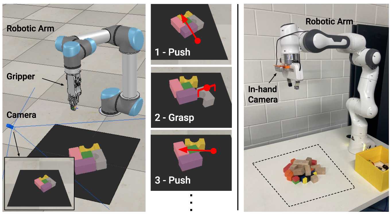
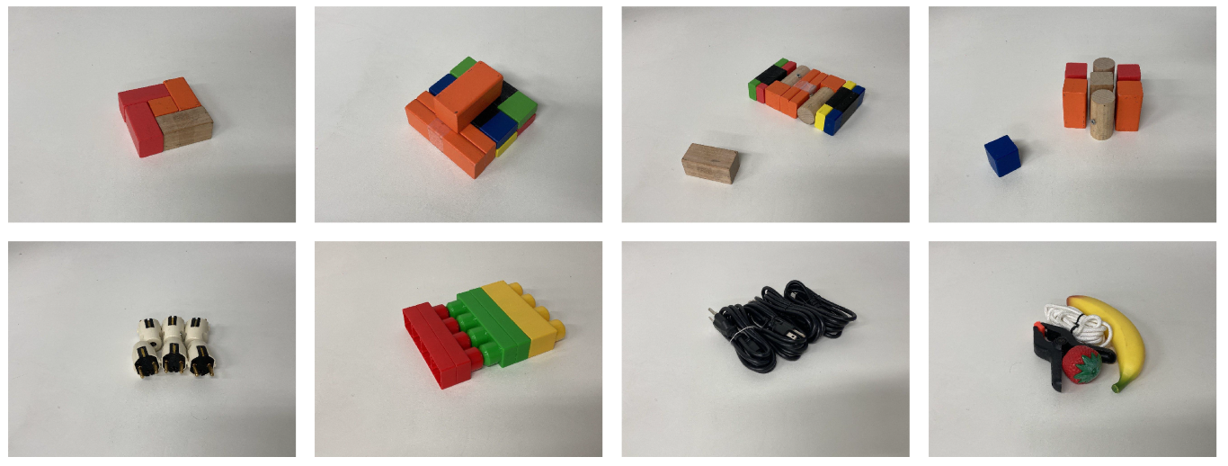
2.1. Robotic Setups
2.2. Problem Formulation
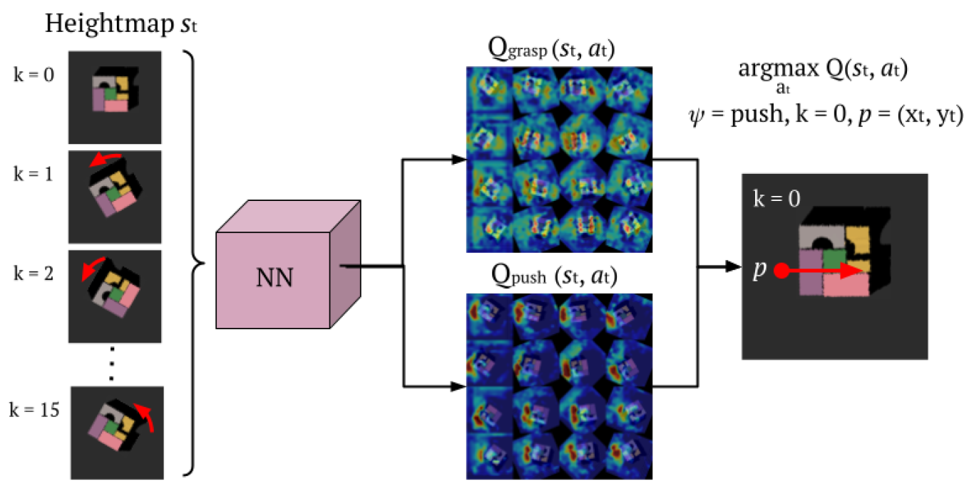
2.2.1. Actions
2.2.2. Rewards
2.3. Processing Pipeline
2.4. Training
2.5. Testing
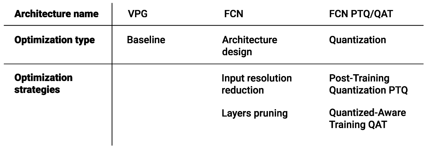
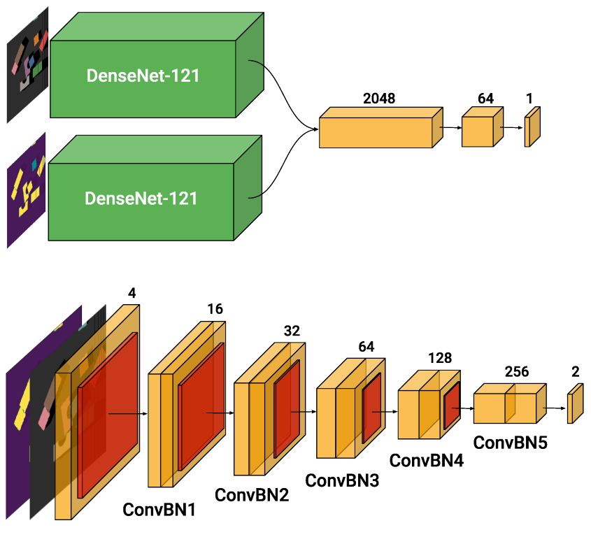
2.6. Architectures
2.6.1. Baseline
2.6.2. Single-FCN
2.7. Input Resolution
2.8. Quantization
2.8.1. Post-Training Quantization
- Fusing; Since we are considering a static model, it is beneficial to fold the batch normalization layers into the convolutional layer. Besides reducing the computational overhead of the additional scaling and offset, this prevents extra data movement.
- Calibration; The network is fed with random samples from the training dataset, for which we track the maximum and minimum values both at weight level and activation level. These values are instrumental for determining the maximum and minimum of the range r.
- Deployment; The weights of the model are finally quantized. At every forward pass, the input of the model is quantized and then fed to the network. The output of the model is then de-quantized to the initial floating-point notation.
2.8.2. Quantization-Aware Training
2.9. Closed-Loop Control
3. Results
3.1. Metrics
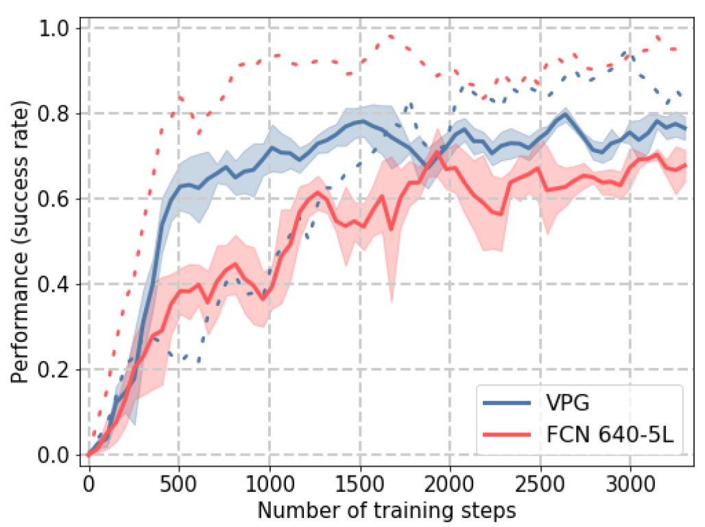
3.2. Training
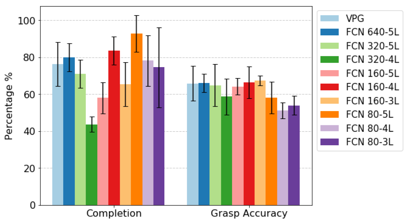
3.3. Testing
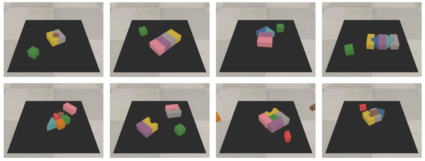
Simulation Environment
3.4. Computation Time
Real Environment
3.5. Closed Loop
4. Discussion
Supplementary Materials
Author Contributions
Funding
Institutional Review Board Statement
Informed Consent Statement
Data Availability Statement
Conflicts of Interest
References
- Popov, I.; Heess, N.; Lillicrap, T.; Hafner, R.; Barth-Maron, G.; Vecerik, M.; Lampe, T.; Tassa, Y.; Erez, T.; Riedmiller, M. Data-efficient Deep Reinforcement Learning for Dexterous Manipulation. arXiv 2017, arXiv:1704.03073. [Google Scholar]
- OpenAI; Akkaya, I.; Andrychowicz, M.; Chociej, M.; Litwin, M.; McGrew, B.; Petron, A.; Paino, A.; Plappert, M.; Powell, G.; et al. Solving Rubik’s Cube with a Robot Hand. arXiv 2019, arXiv:1910.07113. [Google Scholar] [CrossRef]
- Kalashnikov, D.; Irpan, A.; Pastor, P.; Ibarz, J.; Herzog, A.; Jang, E.; Quillen, D.; Holly, E.; Kalakrishnan, M.; Vanhoucke, V.; et al. QT-Opt: Scalable Deep Reinforcement Learning for Vision-Based Robotic Manipulation. arXiv 2018, arXiv:1806.10293. [Google Scholar]
- Pierson, H.A.; Gashler, M.S. Deep learning in robotics: A review of recent research. Adv. Robot. 2017, 31, 821–835. [Google Scholar] [CrossRef]
- LeCun, Y.; Bengio, Y.; Hinton, G. Deep Learning. Nature 2015, 521, 436–444. [Google Scholar] [CrossRef]
- Garcia, C.; Delakis, M. Convolutional face finder: A neural architecture for fast and robust face detection. Pattern Anal. Mach. Intell. IEEE Trans. 2004, 26, 1408–1423. [Google Scholar] [CrossRef]
- Ebert, F.; Dasari, S.; Lee, A.X.; Levine, S.; Finn, C. Robustness via retrying: Closed-loop robotic manipulation with self-supervised learning. In Proceedings of the 2nd Annual Conference on Robot Learning (CoRL 2018), Zurich, Switzerland, 29–31 October 2018; pp. 983–993. [Google Scholar]
- Obando-Ceron, J.S.; Castro, P.S. Revisiting Rainbow: Promoting more Insightful and Inclusive Deep Reinforcement Learning Research. arXiv 2021, arXiv:2011.14826. [Google Scholar]
- Boons, B.; Verhelst, M.; Karsmakers, P. Low power on-line machine monitoring at the edge. In Proceedings of the 2021 International Conference on Applied Artificial Intelligence (ICAPAI), Halden, Norway, 19–21 May 2021; pp. 1–8. [Google Scholar] [CrossRef]
- Zimmermann, C.; Welschehold, T.; Dornhege, C.; Burgard, W.; Brox, T. 3D human pose estimation in rgbd images for robotic task learning. In Proceedings of the 2018 IEEE International Conference on Robotics and Automation (ICRA), Brisbane, Australia, 21–25 May 2018; pp. 1986–1992. [Google Scholar]
- Colomé, A.; Torras, C. Closed-loop inverse kinematics for redundant robots: Comparative assessment and two enhancements. IEEE/ASME Trans. Mechatron. 2014, 20, 944–955. [Google Scholar] [CrossRef]
- Zeng, A.; Song, S.; Welker, S.; Lee, J.; Rodriguez, A.; Funkhouser, T. Learning Synergies between Pushing and Grasping with Self-supervised Deep Reinforcement Learning. In Proceedings of the IEEE/RSJ International Conference on Intelligent Robots and Systems (IROS), Madrid, Spain, 1–5 October 2018. [Google Scholar]
- Károly, A.I.; Elek, R.N.; Haidegger, T.; Széll, K.; Galambos, P. Optical flow-based segmentation of moving objects for mobile robot navigation using pre-trained deep learning models. In Proceedings of the 2019 IEEE International Conference on Systems, Man and Cybernetics (SMC), Bari, Italy, 6–9 October 2019; pp. 3080–3086. [Google Scholar]
- Peters, M.E.; Ruder, S.; Smith, N.A. To tune or not to tune? Adapting pretrained representations to diverse tasks. arXiv 2019, arXiv:1903.05987. [Google Scholar]
- De Coninck, E.; Verbelen, T.; Van Molle, P.; Simoens, P.; Dhoedt, B. Learning robots to grasp by demonstration. Robot. Auton. Syst. 2020, 127, 103474. [Google Scholar] [CrossRef]
- Chen, J.; Ran, X. Deep Learning With Edge Computing: A Review. Proc. IEEE 2019, 107, 1655–1674. [Google Scholar] [CrossRef]
- Murshed, M.G.S.; Murphy, C.; Hou, D.; Khan, N.; Ananthanarayanan, G.; Hussain, F. Machine Learning at the Network Edge: A Survey. ACM Comput. Surv. 2022, 54, 170. [Google Scholar] [CrossRef]
- Howard, A.G.; Zhu, M.; Chen, B.; Kalenichenko, D.; Wang, W.; Weyand, T.; Andreetto, M.; Adam, H. MobileNets: Efficient Convolutional Neural Networks for Mobile Vision Applications. arXiv 2017, arXiv:1704.04861. [Google Scholar]
- Nagel, M.; Fournarakis, M.; Amjad, R.A.; Bondarenko, Y.; van Baalen, M.; Blankevoort, T. A White Paper on Neural Network Quantization. arXiv 2021, arXiv:2106.08295. [Google Scholar]
- Banner, R.; Nahshan, Y.; Hoffer, E.; Soudry, D. Post-Training 4-Bit Quantization of Convolution Networks for Rapid-Deployment. arXiv 2019, arXiv:1810.05723. [Google Scholar]
- Leroux, S.; Vankeirsbilck, B.; Verbelen, T.; Simoens, P.; Dhoedt, B. Training Binary Neural Networks With Knowledge Transfer. Neurocomputing 2019, 396, 534–541. [Google Scholar] [CrossRef]
- Raghuraman, K. Quantizing deep convolutional networks for efficient inference: A whitepaper. arXiv 2018, arXiv:1806.08342. [Google Scholar]
- Rohmer, E.; Singh, S.P.N.; Freese, M. V-REP: A versatile and scalable robot simulation framework. In Proceedings of the 2013 IEEE/RSJ International Conference on Intelligent Robots and Systems, Tokyo, Japan, 3–7 November 2013; pp. 1321–1326. [Google Scholar] [CrossRef]
- Van de Maele, T.; Verbelen, T.; Çatal, O.; De Boom, C.; Dhoedt, B. Active Vision for Robot Manipulators Using the Free Energy Principle. Front. Neurorobotics 2021, 15, 642780. [Google Scholar] [CrossRef]
- Mnih, V.; Kavukcuoglu, K.; Silver, D.; Rusu, A.A.; Veness, J.; Bellemare, M.G.; Graves, A.; Riedmiller, M.; Fidjeland, A.K.; Ostrovski, G.; et al. Human-level control through deep reinforcement learning. Nature 2015, 518, 529–533. [Google Scholar] [CrossRef]
- Schaul, T.; Quan, J.; Antonoglou, I.; Silver, D. Prioritized Experience Replay. arXiv 2016. [Google Scholar] [CrossRef]
- Huang, G.; Liu, Z.; van der Maaten, L.; Weinberger, K.Q. Densely Connected Convolutional Networks. In Proceedings of the 2017 IEEE Conference on Computer Vision and Pattern Recognition (CVPR), Honolulu, HI, USA, 21–26 July 2017. [Google Scholar]
- Ioffe, S.; Szegedy, C. Batch Normalization: Accelerating Deep Network Training by Reducing Internal Covariate Shift. In Proceedings of the 32nd International Conference on International Conference on Machine Learning, Lille, France, 6–11 July 2015; Volume 37, pp. 448–456. [Google Scholar]
- Krishnan, S.; Lam, M.; Chitlangia, S.; Wan, Z.; Barth-Maron, G.; Faust, A.; Reddi, V.J. QuaRL: Quantization for Sustainable Reinforcement Learning. arXiv 2021, arXiv:1910.01055. [Google Scholar]
- Paszke, A.; Gross, S.; Massa, F.; Lerer, A.; Bradbury, J.; Chanan, G.; Killeen, T.; Lin, Z.; Gimelshein, N.; Antiga, L.; et al. PyTorch: An Imperative Style, High-Performance Deep Learning Library. In Advances in Neural Information Processing Systems 32: Annual Conference on Neural Information Processing Systems 2019, NeurIPS 2019, 8–14 December 2019, Vancouver, BC, Canada; Wallach, H., Larochelle, H., Beygelzimer, A., d’Alché-Buc, F., Fox, E., Garnett, R., Eds.; Curran Associates, Inc.: Red Hook, NY, USA, 2019; pp. 8024–8035. [Google Scholar]
- Yoshua Bengio, N.L.; Courville, A. Estimating or propagating gradients through stochastic neurons for conditional computation. arXiv 2013, arXiv:1308.3432. [Google Scholar]
- Kaspar, M.; Osorio, J.D.M.; Bock, J. Sim2Real Transfer for Reinforcement Learning without Dynamics Randomization. In Proceedings of the 2020 IEEE/RSJ International Conference on Intelligent Robots and Systems (IROS), Las Vegas, NV, USA, 24 October 2020–24 January 2021. [Google Scholar]
- Zhao, W.; Queralta, J.P.; Westerlund, T. Sim-to-Real Transfer in Deep Reinforcement Learning for Robotics: A Survey. In Proceedings of the 2020 IEEE Symposium Series on Computational Intelligence (SSCI), Canberra, Australia, 1–4 December 2020. [Google Scholar]


| Resolution | 5 Layer Blocks (5L) | 4 Layer Blocks (4L) | 3 Layer Blocks (3L) |
|---|---|---|---|
| 640 × 640 | 3.49 G | - | - |
| 320 × 320 | 1.14 G | 2.43 G | - |
| 160 × 160 | 616.66 M | 872.66 M | 1.4 G |
| 80 × 80 | 532.18 M | 550.1 M | 616.66 M |
| Methods | Grasp Accuracy % | Action Efficiency % | Completion % |
|---|---|---|---|
| FCN 160-4L | 66.4 ± 8.5 | 47.3 ± 5.2 | 83.6 ± 7.6 |
| FCN 160-4L PTQ | 65.3 ± 2.9 | 51.4 ± 6.5 | 85.4 ± 10.4 |
| Methods | Grasp Accuracy % | Action Efficiency % | Completion % |
|---|---|---|---|
| FCN 160-4L | 56.4 | 50.0 | 100.0 |
| FCN 160-4L PTQ | 62.0 | 58.3 | 100.0 |
| FCN 160-4L QAT | 57.2 | 49.3 | 100.0 |
| Methods | Grasp Accuracy % | Action Efficiency % | Completion % |
|---|---|---|---|
| FCN 160-4L | 61.5 | 50.0 | 100.0 |
| FCN 160-4L PTQ | 63.9 | 56.8 | 100.0 |
| FCN 160-4L QAT | 64.9 | 53.2 | 100.0 |
Publisher’s Note: MDPI stays neutral with regard to jurisdictional claims in published maps and institutional affiliations. |
© 2022 by the authors. Licensee MDPI, Basel, Switzerland. This article is an open access article distributed under the terms and conditions of the Creative Commons Attribution (CC BY) license (https://creativecommons.org/licenses/by/4.0/).
Share and Cite
Ferraro, S.; Van de Maele, T.; Mazzaglia, P.; Verbelen, T.; Dhoedt, B. Computational Optimization of Image-Based Reinforcement Learning for Robotics. Sensors 2022, 22, 7382. https://doi.org/10.3390/s22197382
Ferraro S, Van de Maele T, Mazzaglia P, Verbelen T, Dhoedt B. Computational Optimization of Image-Based Reinforcement Learning for Robotics. Sensors. 2022; 22(19):7382. https://doi.org/10.3390/s22197382
Chicago/Turabian StyleFerraro, Stefano, Toon Van de Maele, Pietro Mazzaglia, Tim Verbelen, and Bart Dhoedt. 2022. "Computational Optimization of Image-Based Reinforcement Learning for Robotics" Sensors 22, no. 19: 7382. https://doi.org/10.3390/s22197382
APA StyleFerraro, S., Van de Maele, T., Mazzaglia, P., Verbelen, T., & Dhoedt, B. (2022). Computational Optimization of Image-Based Reinforcement Learning for Robotics. Sensors, 22(19), 7382. https://doi.org/10.3390/s22197382