

A Novel and Non-Invasive Approach to Evaluating Soil Moisture without Soil Disturbances: Contactless Ultrasonic System


Abstract
:1. Introduction
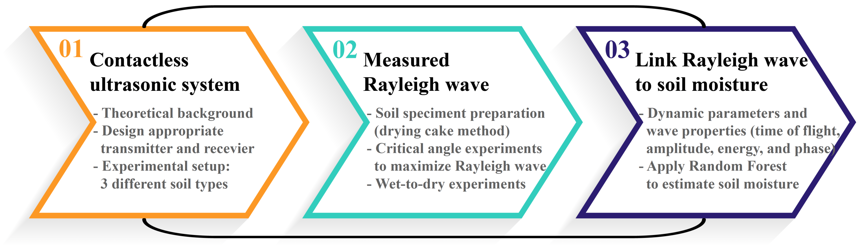
2. Method
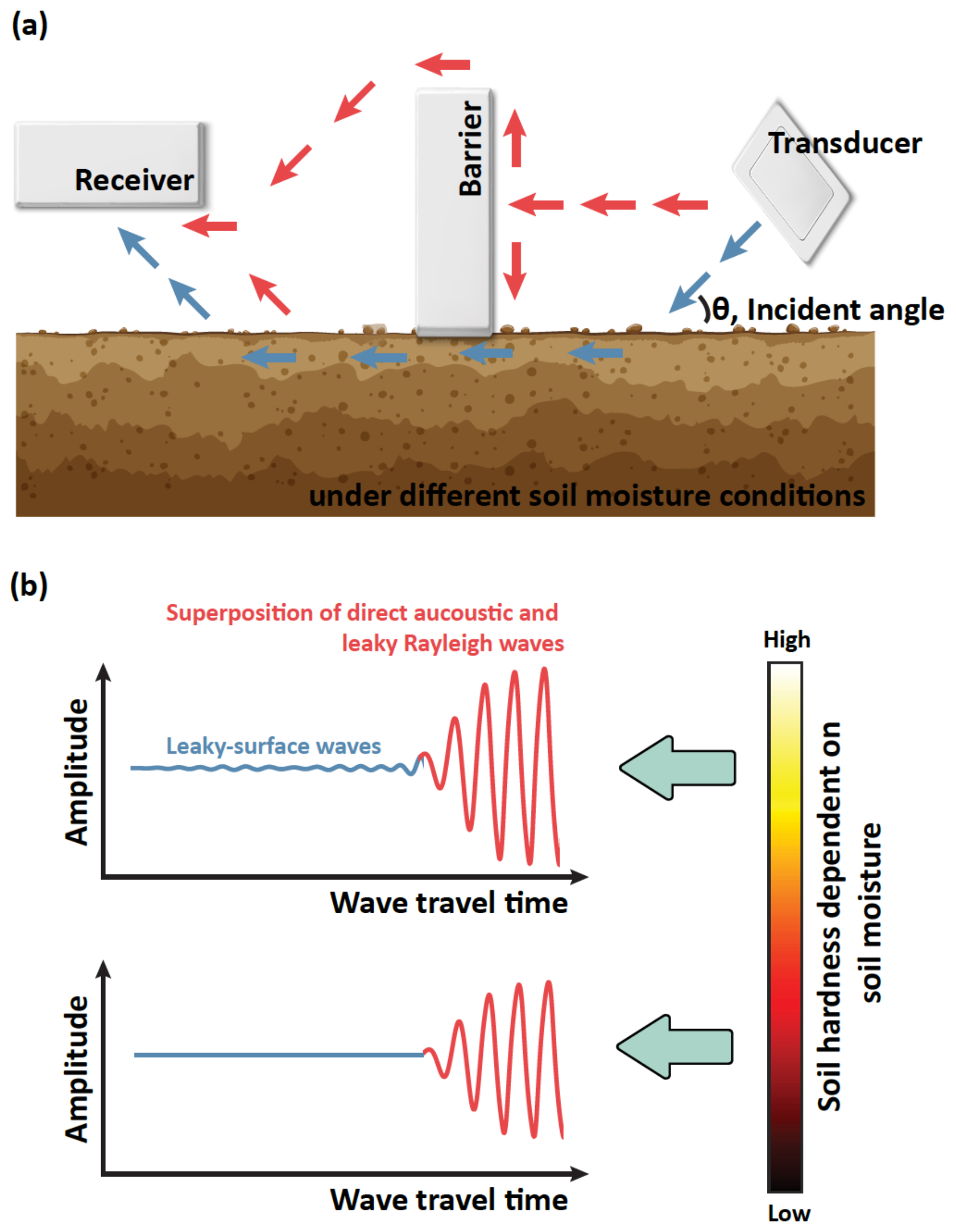
2.1. Theoretical Background of Rayleigh Wave
2.2. Contactless Ultrasonic System
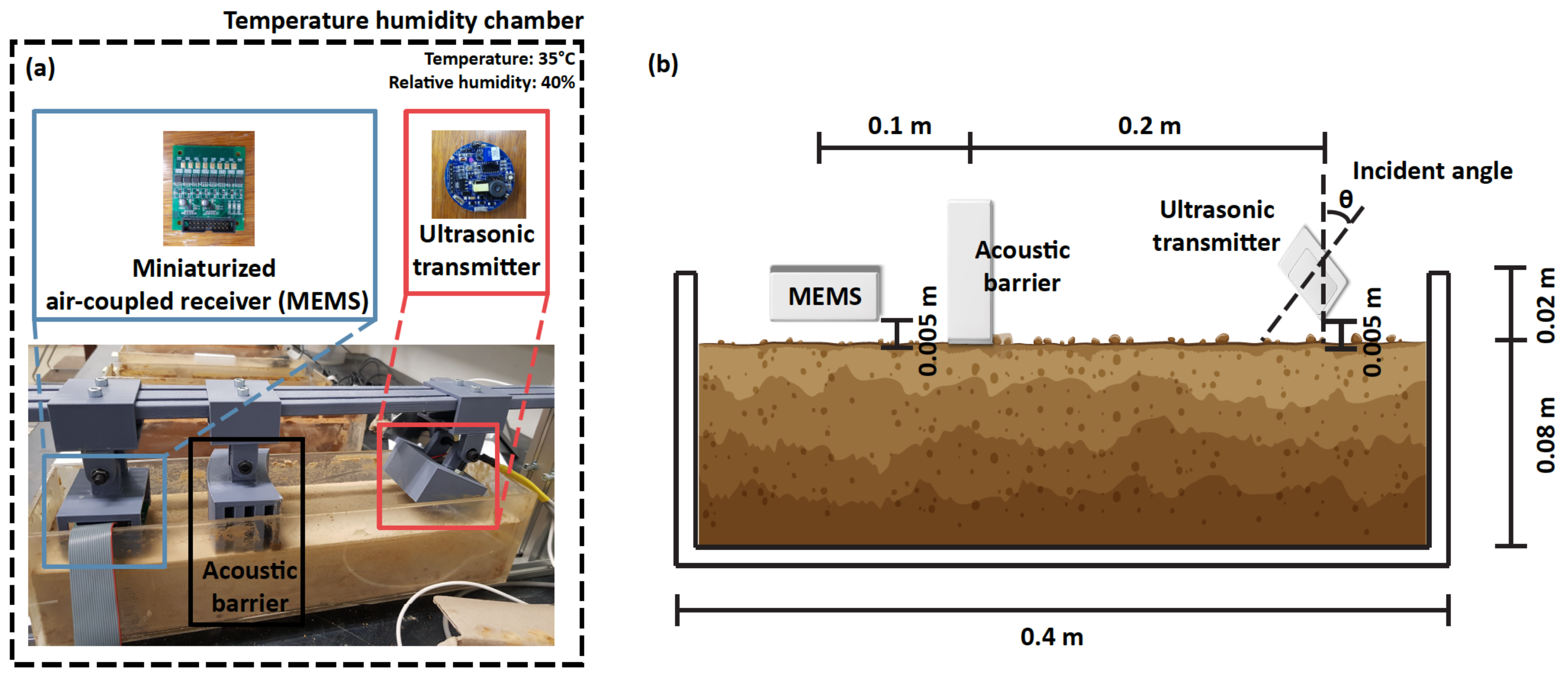
2.3. Experimental Setup
2.4. Random Forests
3. Results
3.1. Critical Angle Experiment
3.2. Dynamic Parameters Dependent on Soil Moisture
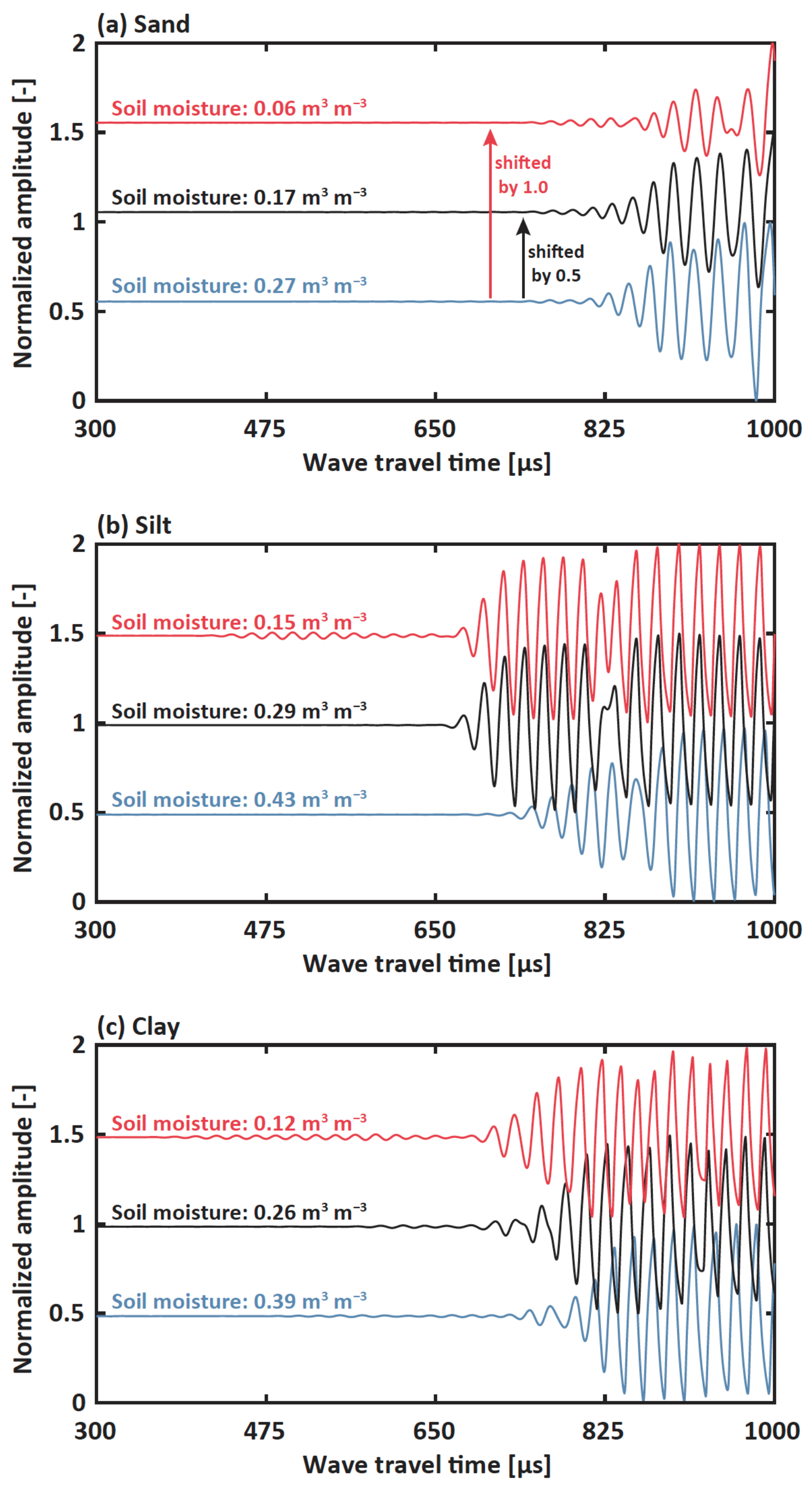
3.3. Wave Properties Dependent on Soil Moisture
3.4. Soil Moisture Prediction Using Random Forests
4. Discussion
5. Conclusions
- The ultrasonic system developed in this study was able to clearly detect the changes in surface soil moisture through the excitation and reception of leaky Rayleigh waves.
- Strong relationships were identified between the energy and amplitude of leaky Rayleigh waves and soil moisture for the three tested soil types (sand, silt, and clay).
- The proposed deep learning approach showed the accurate and robust estimations of soil moisture using the dynamic parameters and wave properties of the observed leaky Rayleigh waves for the validation and test datasets, regardless of the soil texture and soil moisture contents (R ≥ 0.98, RMSE ≤ 0.0089 m m).
Author Contributions
Funding
Institutional Review Board Statement
Informed Consent Statement
Data Availability Statement
Conflicts of Interest
References
- Sung, S.G.; Lee, I.M.; Cho, G.C.; Reddi, L.N. Estimation of soil-water characteristics using liquid limit state. Géotechnique 2006, 55, 569–573. [Google Scholar] [CrossRef]
- Simms, P.H.; Yanful, E.K. Predicting soil–water characteristic curves of compacted plastic soils from measured pore-size distributions. Géotechnique 2002, 52, 269–278. [Google Scholar] [CrossRef]
- Wang, C.; Fu, B.; Zhang, L.; Xu, Z. Soil moisture-plant interactions: An ecohydrological review. Front. Soils Sediments 2019, 19, 1–9. [Google Scholar] [CrossRef]
- Daly, E.; Porporato, A. A Review of Soil Moisture Dynamics: From Rainfall Infiltration to Ecosystem Response. Environ. Eng. Sci. 2005, 22, 9–24. [Google Scholar] [CrossRef]
- Drewry, D.T.; Kumar, P.; Long, S.; Bernacchi, C.; Liang, X.Z.; Sivapalan, M. Ecohydrological responses of dense canopies to environmental variability: 1. Interplay between vertical structure and photosynthetic pathway. J. Geophys. Res. 2010, 115, G04002. [Google Scholar] [CrossRef]
- Cepuder, P.; Nolz, R. Irrigation management by means of soil moisture sensortechnologies. J. Water Land Dev. 2007, 11, 79–90. [Google Scholar] [CrossRef]
- Millan, S.; Casadesus, J.; Campillo, C.; Monino, M.J.; Prieto, M.H. Using Soil Moisture Sensors for Automated Irrigation Scheduling in a Plum Crop. Water 2019, 11, 2061. [Google Scholar] [CrossRef]
- Porporato, A.; D’Odorico, P.; Laio, F.; Rodriguez-Iturbe, I. Hydrologic controls on soil carbon and nitrogen cycles. I. Modeling scheme. Adv. Water Resour. 2003, 26, 45–58. [Google Scholar] [CrossRef]
- Woo, D.K.; Quijano, J.C.; Kumar, P.; Chaoka, S.; Bernacchi, C.J. Threshold dynamics in soil carbon storage for bioenergy crops. Environ. Sci. Technol. 2014, 48, 12090–12098. [Google Scholar] [CrossRef]
- Woo, D.K.; Kumar, P. Impacts of Subsurface Tile Drainage on Age–Concentration Dynamics of Inorganic Nitrogen in Soil. Water Resour. Res. 2019, 55, 1470–1789. [Google Scholar] [CrossRef]
- Reiners, W.A. Carbon Dioxide Evolution from the Floor of Three Minnesota Forests. Ecology 1968, 49, 471–483. [Google Scholar] [CrossRef]
- Raich, J.W.; Schlesinger, W.H. The global carbon dioxide flux in soil respiration and its relationship to vegetation and climate. Tellus B Chem. Phys. Meteorol. 1992, 44, 81–99. [Google Scholar] [CrossRef]
- Hillel, D. Introduction to Soil Physics; Academic Press: Orlando, FL, USA, 1982. [Google Scholar] [CrossRef]
- Robinson, D.A.; Campbell, C.S.; Hopmans, J.W.; Hornbuckle, B.K.; Jones, S.B.; Knight, R.; Ogden, F.; Selker, J.; Wendroth, O. Soil Moisture Measurement for Ecological and Hydrological Watershed-Scale Observatories: A Review. Vadose Zone J. 2008, 7, 358–389. [Google Scholar] [CrossRef]
- SU, S.L.; Singh, D.; Shojaei Baghini, M. A critical review of soil moisture measurement. Measurement 2014, 54, 92–105. [Google Scholar] [CrossRef]
- Jackson, P.; Northmore, K.; Meldrum, P.; Gunn, D.; Hallam, J.; Wambura, J.; Wangusi, B.; Ogutu, G. Non-invasive moisture monitoring within an earth embankment—A precursor to failure. NDT E Int. 2002, 35, 107–115. [Google Scholar] [CrossRef]
- Sayde, C.; Gregory, C.; Gil-Rodriguez, M.; Tufillaro, N.; Tyler, S.; van de Giesen, N.; English, M.; Cuenca, R.; Selker, J.S. Feasibility of soil moisture monitoring with heated fiber optics. Water Resour. Res. 2010, 46, W06201. [Google Scholar] [CrossRef]
- Pires, L.F.; Bacchi, O.O.; Reichardt, K. Soil water retention curve determined by gamma-ray beam attenuation. Soil Tillage Res. 2005, 82, 89–97. [Google Scholar] [CrossRef]
- Fityus, S.; Wells, T.; Huang, W. Water Content Measurement in Expansive Soils Using the Neutron Probe. Geotech. Test. J. 2011, 34, 102828. [Google Scholar] [CrossRef]
- Klotzsche, A.; Jonard, F.; Looms, M.C.; van der Kruk, J.; Huisman, J. Measuring Soil Water Contentwith Ground Penetrating Radar:A Decade of Progress. Vadose Zone J. 2018, 17, 180052. [Google Scholar] [CrossRef] [Green Version]
- Wu, K.; Gabriela Arambulo, R.; Zajc, M.; Jacquemin, E.; Clement, M.; Coster, A.D.; Lambot, S. A new drone-borne GPR for soil moisture mapping. Remote Sens. Environ. 2019, 235, 111456. [Google Scholar] [CrossRef]
- Coutinho, R.M.; Sousa, A.; Santos, F.; Cunha, M. Contactless Soil Moisture Mapping Using InexpensiveFrequency-Modulated Continuous Wave RADAR forAgricultural Purposes. Appl. Sci. 2022, 12, 5471. [Google Scholar] [CrossRef]
- Binley, A.; Winship, P.; West, L.J.; Pokar, M.; Middleton, R. Sea-sonal variation of moisture content in unsaturated sandstone inferred from borehole radar and resistivity profiles. J. Hydrol. 2002, 267, 160–172. [Google Scholar] [CrossRef]
- Zhang, X.; Davidson, E.A.; Mauzerall, D.L.; Searchinger, T.D.; Dumas, P.; She, Y. Managing nitrogen for sustainable development. Nature 2015, 528, 51–59. [Google Scholar] [CrossRef] [PubMed]
- Sharma, R.K.; Gupta, A.K. Continuous wave acoustic method for determination of moisture content in agricultural soil. Comput. Electron. Agric. 2010, 73, 105–111. [Google Scholar] [CrossRef]
- Flammer, I.; Blum, A.; Leiser, A.; Germann, P. Acoustic assessment of flow patterns in unsaturated soil. J. Appl. Geophys. 2001, 46, 115–128. [Google Scholar] [CrossRef]
- Oelze, M.L.; O’Brien, W.D.; Darmody, R.G. Measurement of Attenuation and Speed of Sound in Soils. Soil Sci. Soc. Am. J. 2002, 66, 788–796. [Google Scholar] [CrossRef]
- Lo, W.C.; Yeh, C.L.; Tsai, C.T. Effect of soil texture on the propagation and attenuation of acoustic wave at unsaturated conditions. J. Hydrol. 2007, 338, 273–284. [Google Scholar] [CrossRef]
- Chimenti, D.E. Review of air-coupled ultrasonic materials characterization. Ultrasonics 2014, 54, 1804–1816. [Google Scholar] [CrossRef]
- Lin, S.; Ashlock, J.; Li, B. Direct estimation of shear-wave velocity profiles from surface wave investigation of geotechnical sites. Géotechnique 2021, 1–9. [Google Scholar] [CrossRef]
- Lin, W.; Mao, W.; Liu, A.; Koseki, J. Application of an acoustic emission source-tracing method to visualise shear banding in granular materials. Géotechnique 2021, 71, 925–936. [Google Scholar] [CrossRef]
- Zamen, S.; Dehghan-Niri, E.; Al-Beer, H.; Lindahl, J.; Hassen, A.A. Characterization of nonlinear ultrasonic waves behavior while interacting with poor interlayer bonds in large-scale additive manufactured materials. NDT E Int. 2022, 127, 102602. [Google Scholar] [CrossRef]
- Hong, J.; Kim, R.; Hoon, C.; Chooi, H. Evaluation of stiffening behavior of concrete based on contactless ultrasonic system and maturity method. Constr. Build. Mater. 2020, 262, 120717. [Google Scholar] [CrossRef]
- Hong, J.; Choi, H. Monitoring Hardening Behavior of Cementitious Materials Using Contactless Ultrasonic Method. Sensors 2021, 21, 3421. [Google Scholar] [CrossRef]
- Viktorov, I.A. Rayleigh and Lamb Waves; Springer: Berlin/Heidelberg, Germany, 1967. [Google Scholar]
- Declercq, N.F.; Lamkanfi, E. Study by means of liquid side acoustic barrier of the influence of leaky Rayleigh waves on bounded beam reflection. Appl. Phys. Lett. 2008, 93, 054103. [Google Scholar] [CrossRef]
- Lamkanfi, E.; Declercq, N.F.; Paepegem, W.V.; Degrieck, J. Numerical study of Rayleigh wave transmission through an acoustic barrier. J. Apllied Phys. 2009, 105, 114902. [Google Scholar] [CrossRef]
- Soil Survey Staff. Keys to Soil Taxonomy; USDA Natural Resources Conservation Service: Washington, DC, USA, 2010. [Google Scholar]
- van Genuchten, M.T. A cloased-form equation for predicting the hydraulic conductivity of unsaturated soils. Soil Sci. Soc. Am. J. 1980, 44, 892–898. [Google Scholar] [CrossRef]
- Kramer, P.; Boyer, J. Water Relations of Plants and Soils; New York Academic Press: New York, NY, USA, 1983. [Google Scholar]
- Essien, U.E.; Akankpo, A.; Igboekwe, M. Poisson’s Ratio of Surface Soils and Shallow Sediments Determined from Seismic Compressional and Shear Wave Velocities. Int. J. Geosci. 2014, 5, 1540–1546. [Google Scholar] [CrossRef]
- Payan, M.; Khoshini, M.; Chenari, R.J. Elastic Dynamic Young’s Modulus and Poisson’s Ratio of Sand-Silt Mixtures. J. Mater. Civ. Eng. 2019, 32, 04019314. [Google Scholar] [CrossRef]
- Graff, K.F. Wave Motion in Elastic Solids; Dover Publications, Inc.: New York, NY, USA, 1975. [Google Scholar]
- Lu, N.; Kaya, M. A Drying Cake Method for Measuring Suction-Stress Characteristic Curve, Soil-Water-Retention Curve, and Hydraulic Conductivity Function. Geotech. Test. J. 2013, 36, 20120097. [Google Scholar] [CrossRef]
- Breiman, L. Random Forests. Mach. Learn. 2001, 45, 5–32. [Google Scholar] [CrossRef]
- Fellman, J.B.; Buma, B.; Hood, E.; Edwards, R.T.; D’Amore, D.V. Linking LiDAR with streamwater biogeochemistry in coastaltemperate rainforest watersheds. Can. J. Fish. Aquat. Sci. 2017, 74, 801–811. [Google Scholar] [CrossRef]
- Guo, X.; Bian, Z.; Wang, S.; Wang, Q.; Zhang, Y.; Zhou, J.; Lin, L. Prediction of the spatial distribution of soil arthropods using a random forest model: A case study in Changtu County, Northeast China. Agric. Ecosyst. Environ. 2020, 292, 106818. [Google Scholar] [CrossRef]
- Perie, C.; de Blois, S. Dominant forest tree species are potentially vulnerable to climate change over large portions of their range even at high latitudes. PeerJ 2016, 4, e2218. [Google Scholar] [CrossRef]
- Rather, T.A.; Kumar, S.; Khan, J.A. Using machine learning to predict habitat suitability of sloth bears at multiple spatial scales. Ecol. Process. 2021, 10, 48. [Google Scholar] [CrossRef]
- Tongal, H.; Booij, M.J. Simulation and forecasting of streamflows using machine learning models coupled with base flow separation. J. Hydrol. 2018, 564, 266–282. [Google Scholar] [CrossRef]
- Pham, L.T.; Luo, L.; Finley, A. Evaluation of random forests for short-term daily streamflow forecasting in rainfall- and snowmelt-driven watersheds. Hydrol. Earth Syst. Sci. 2021, 25, 2997–3015. [Google Scholar] [CrossRef]
- Desai, S.; Ouarda, T.B. Regional hydrological frequency analysis at ungauged sites with random forest regression. J. Hydrol. 2020, 594, 125861. [Google Scholar] [CrossRef]
- Bagheri, A.R.; Ghaedi, M.; Hajati, S.; Ghaedi, A.M.; Goudarzid, A.; Asfarama, A. Random forest model for the ultrasonic-assisted removal of chrysoidine G by copper sulfide nanoparticles loaded on activated carbon; response surface methodology approach. RSC Adv. 2015, 5, 59335–59343. [Google Scholar] [CrossRef]
- Farinas, M.D.; Jimenez-Carretero, D.; Sancho-Knapik, D.; Peguero-Pina, J.J.; Gil-Pelegrin, E.; Alvarez-Arenas, T.G. Instantaneous and non-destructive relative water content estimation from deep learning applied to resonant ultrasonic spectra of plant leaves. Plant Methods 2019, 15, 218. [Google Scholar] [CrossRef]
- Rodriguez-Galiano, V.F.; Chica-Rivas, M. Evaluation of different machine learning methods for land cover mapping of a Mediterranean area using multi-seasonal Landsat images and Digital Terrain Models. Int. J. Digit. Earth 2014, 7, 492–509. [Google Scholar] [CrossRef]
- Lay, T.; Wallace, T.C. Chapter 4—Surface Waves and Free Oscillations. Int. Geophys. 1995, 58, 116–172. [Google Scholar] [CrossRef]
- Lee, K.; Kim, J.; Lee, C.; Yoon, C.; Choi, J. A Study on the P Wave Arrival Time Determination Algorithm of Acoustic Emission (AE) Suitable for P Waves with Low Signal-to-Noise Ratios. Tunn. Undergr. Space 2011, 21, 249–358. [Google Scholar]
- de Mahieu, A.; Ponette, Q.; Mounir, F.; Lambot, S. Using GPR to analyze regeneration success of cork oaks in the Maamora forest (Morocco). NDT E Int. 2020, 115, 102297. [Google Scholar] [CrossRef]
- Pandey, P.; Lynch, K.; Sivakumar, V.; Solan, B.; Tripathy, S.; Nanda, S.; Donohue, S. Measurements of permeability of saturated and unsaturated soils. Géotechnique 2021, 71, 170–177. [Google Scholar] [CrossRef]
- Sharma, K.; Irmak, S.; Kukal, M.S. Propagation of soil moisture sensing uncertainty into estimation of total soil water, evapotranspiration and irrigation decision-making. Agric. Water Manag. 2021, 243, 106454. [Google Scholar] [CrossRef]
- Yu, L.; Gao, W.; Shamshiri, R.R.; Tao, S.; Ren, Y.; Zhang, Y.; Su, G. Review of research progress on soil moisture sensor technology. Int. J. Agric. Biol. Eng. 2021, 14, 32–42. [Google Scholar] [CrossRef]
- Kitic, G.; Crnojevic-Bengin, V. A sensor for the measurement of the moisture of undisturbed soil samples. Sensors 2013, 13, 1692–1705. [Google Scholar] [CrossRef]
- Datta, S.; Taghvaeian, S.; Ochsner, T.E.; Moriasi, D.; Gowda, P.; Steiner, J.L. Performance Assessment of Five Different Soil Moisture Sensors under Irrigated Field Conditions in Oklahoma. Sensors 2018, 18, 3786. [Google Scholar] [CrossRef]
- de Jong, S.M.; Heijenk, R.A.; Nijland, W.; van der Meijde, M. Monitoring Soil Moisture Dynamics Using Electrical Resistivity Tomography under Homogeneous Field Conditions. Sensors 2020, 20, 5313. [Google Scholar] [CrossRef]
- Mainsant, G.; Jongmans, D.; Chambon, G.; Larose, E.; Baillet, L. Shear-wave velocity as an indicator for rheological changes in clay materials: Lessons from laboratory experiments. Geophys. Res. Lett. 2012, 39, L193601. [Google Scholar] [CrossRef]
- Harba, P.; Pilecki, Z. Assessment of time-spatial changes of shear wave velocities of flysch formation prone to mass movements by seismic interferometry with the use of ambient noise. Landslides 2017, 14, 1225–1233. [Google Scholar] [CrossRef]
- Hussain, Y.; Cardenas-Soto, M.; Moreira, C.; Rodriguez-Rebolledo, J.; Hamza, O.; Prado, R.; Martinez-Carvajal, H.; Dou, J. Variation in Rayleigh wave ellipticity as a possible indicator of earthflow mobility: A case study of Sobradinho landslide compared with pile load testing. Earth Sci. Res. J. 2020, 24, 141–151. [Google Scholar] [CrossRef]
- Mohseni, S.; Payan, M.; Chenari, R.J. Soil-structure interaction analysis in natural heterogeneous deposits using random field theory. Innov. Infrastruct. Solut. 2018, 3, 62. [Google Scholar] [CrossRef]
- Woo, D.K.; Riley, W.J.; Wu, Y. More Fertilizer and Impoverished Roots Required for Improving Wheat Yields and Profits under Climate Change. Field Crop. Res. 2020, 249, 107756. [Google Scholar] [CrossRef]
- Adomako, M.O.; Xue, W.; Roiloa, S.; Zhang, Q.; Du, D.L.; Yu, F.H. Earthworms Modulate Impacts of Soil Heterogeneity on Plant Growth at Different Spatial Scales. Front. Plant Sci. 2021, 12, 735495. [Google Scholar] [CrossRef]
- Sharma, M.D. Rayleigh wave at the surface of a general anisotropic poroelastic medium: Derivation of real secular equation. Proc. R. Soc. A Math. Phys. Eng. Sci. 2018, 471, 20170589. [Google Scholar] [CrossRef]
- Kaur, I.; Lata, P. Rayleigh wave propagation in transversely isotropic magneto-thermoelastic medium with three-phase-lag heat transfer and diffusion. Int. J. Mech. Mater. Eng. 2019, 14, 12. [Google Scholar] [CrossRef]
- Sarris, G.; Haslinger, S.G.; Huthwaite, P.; Nagy, P.B.; Lowe, M.J.S. Attenuation of Rayleigh waves due to surface roughness. J. Acoust. Soc. Am. 2021, 149, 4298. [Google Scholar] [CrossRef]


| Specimen Type | Particle Size | P-Wave Speed | Incident Angle | Porosity |
|---|---|---|---|---|
| Sand | 2.0 to 0.05 mm | 837∼1907 m s | 9.5 | 0.3 |
| Silt | 0.05 to 0.002 mm | 528∼1552 m s | 18.5 | 0.42 |
| Clay | Less than 0.002 mm | 355∼1488 m s | 22 | 0.4 |
Publisher’s Note: MDPI stays neutral with regard to jurisdictional claims in published maps and institutional affiliations. |
© 2022 by the authors. Licensee MDPI, Basel, Switzerland. This article is an open access article distributed under the terms and conditions of the Creative Commons Attribution (CC BY) license (https://creativecommons.org/licenses/by/4.0/).
Share and Cite
Woo, D.K.; Do, W.; Hong, J.; Choi, H. A Novel and Non-Invasive Approach to Evaluating Soil Moisture without Soil Disturbances: Contactless Ultrasonic System. Sensors 2022, 22, 7450. https://doi.org/10.3390/s22197450
Woo DK, Do W, Hong J, Choi H. A Novel and Non-Invasive Approach to Evaluating Soil Moisture without Soil Disturbances: Contactless Ultrasonic System. Sensors. 2022; 22(19):7450. https://doi.org/10.3390/s22197450
Chicago/Turabian StyleWoo, Dong Kook, Wonseok Do, Jinyoung Hong, and Hajin Choi. 2022. "A Novel and Non-Invasive Approach to Evaluating Soil Moisture without Soil Disturbances: Contactless Ultrasonic System" Sensors 22, no. 19: 7450. https://doi.org/10.3390/s22197450
APA StyleWoo, D. K., Do, W., Hong, J., & Choi, H. (2022). A Novel and Non-Invasive Approach to Evaluating Soil Moisture without Soil Disturbances: Contactless Ultrasonic System. Sensors, 22(19), 7450. https://doi.org/10.3390/s22197450