
Requirements for Automotive LiDAR Systems

 , ,
, ,
Abstract
:1. Introduction
2. State of the Art
2.1. Current Requirements for Automotive LiDAR Systems
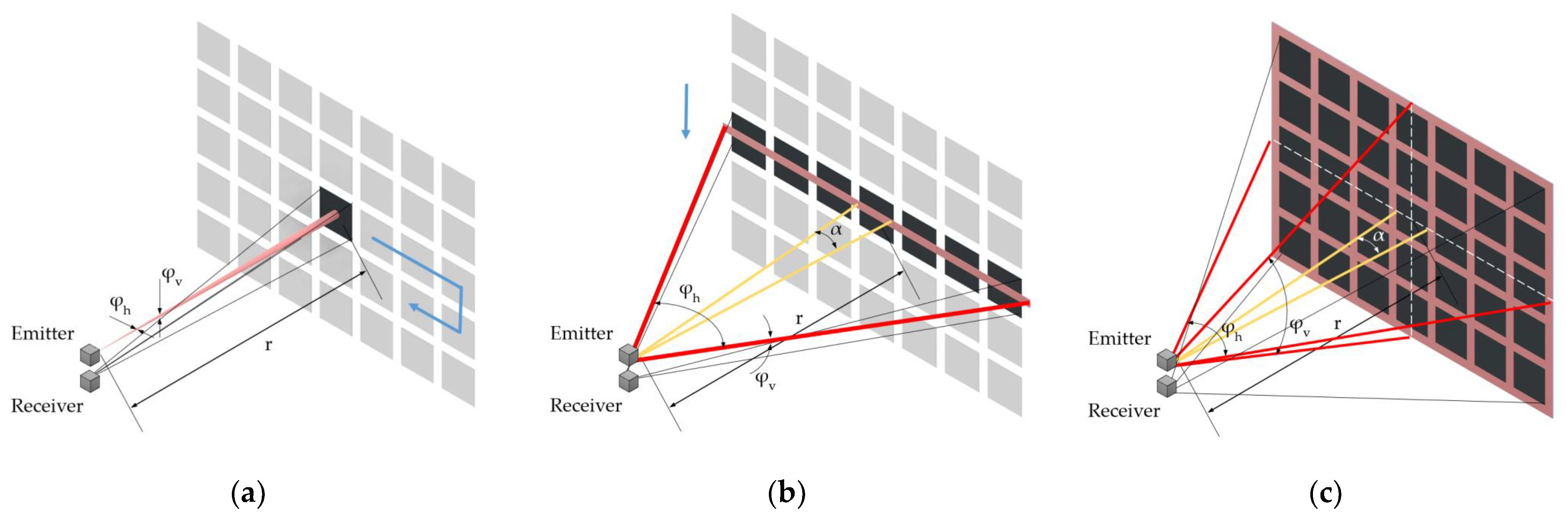
2.2. Functional Principle and Principal Components of LiDAR Systems
3. Range Equation for Different Radiation Patterns
4. Investigation of the Requirements for LiDAR Systems
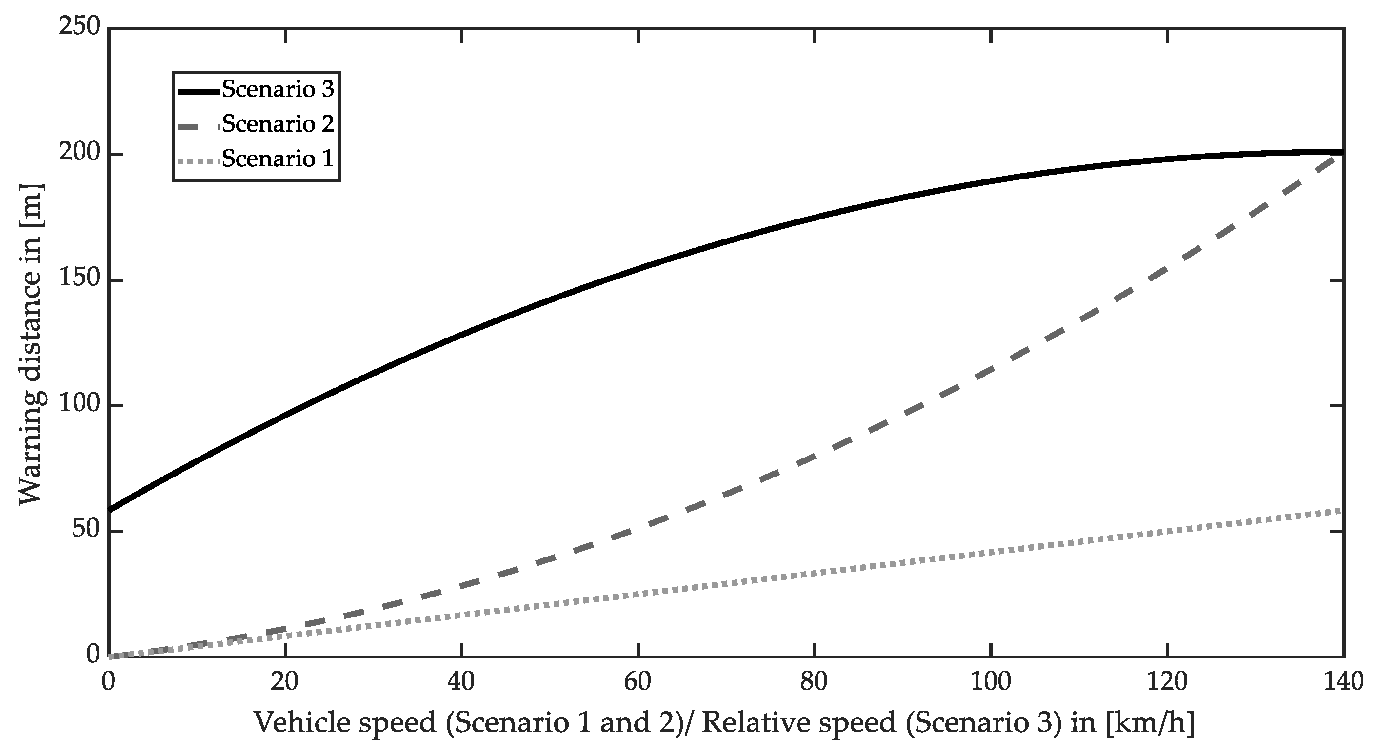
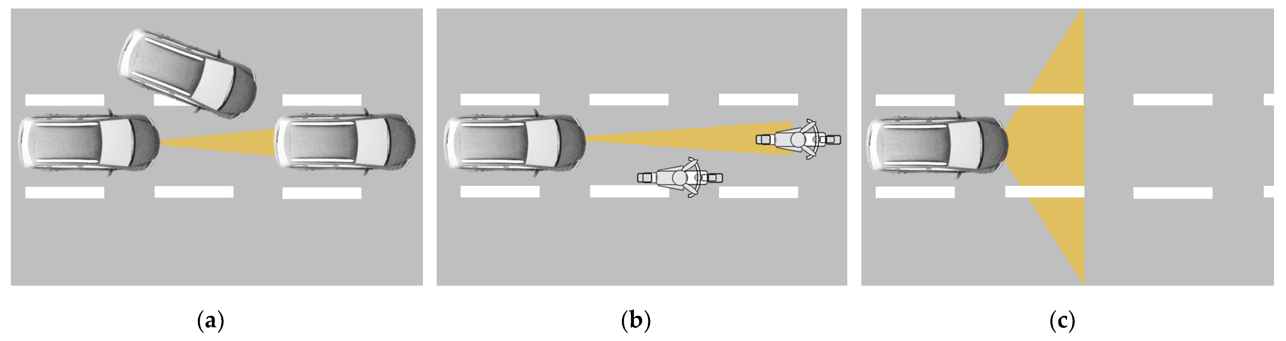
4.1. Detection Range of the ADAS Applications
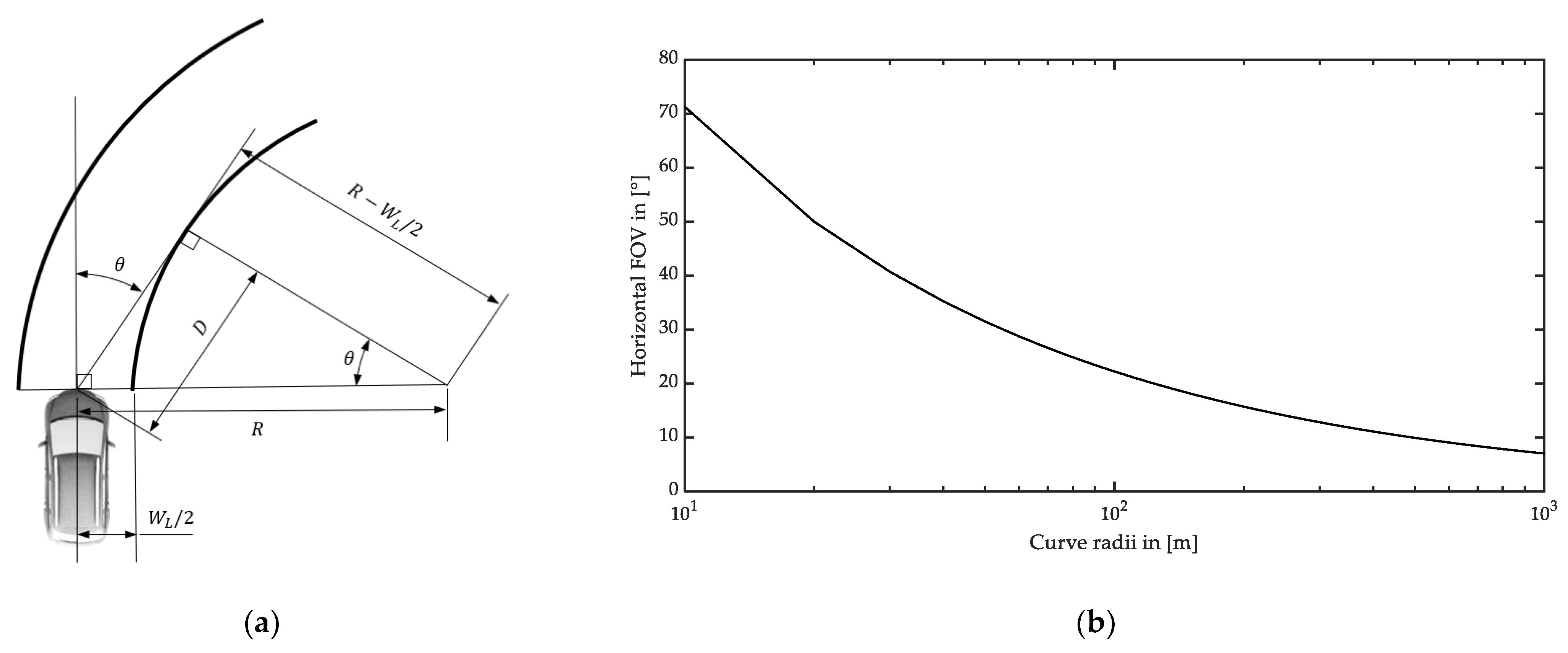
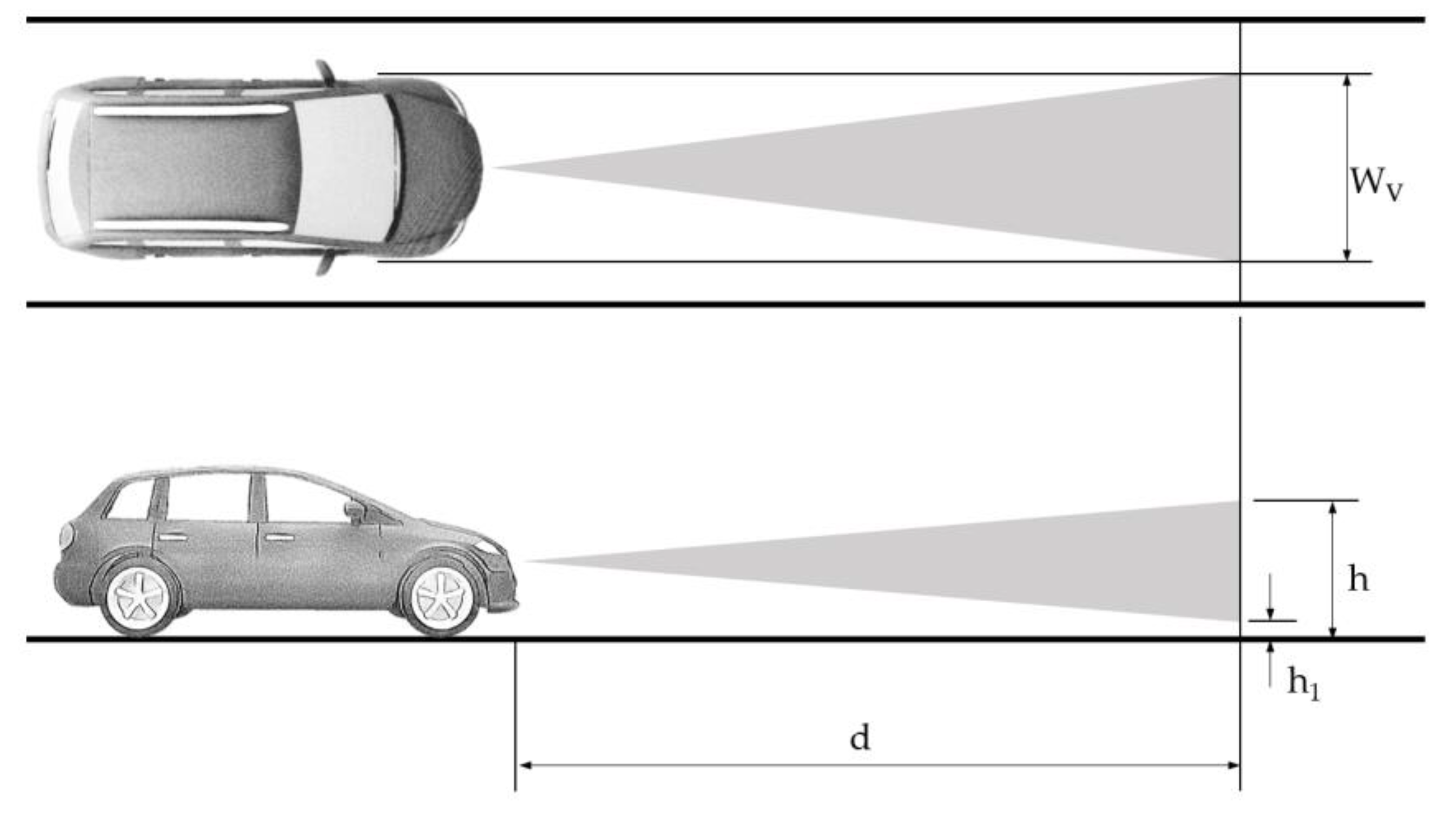
4.2. Field of View Requirements for ADAS
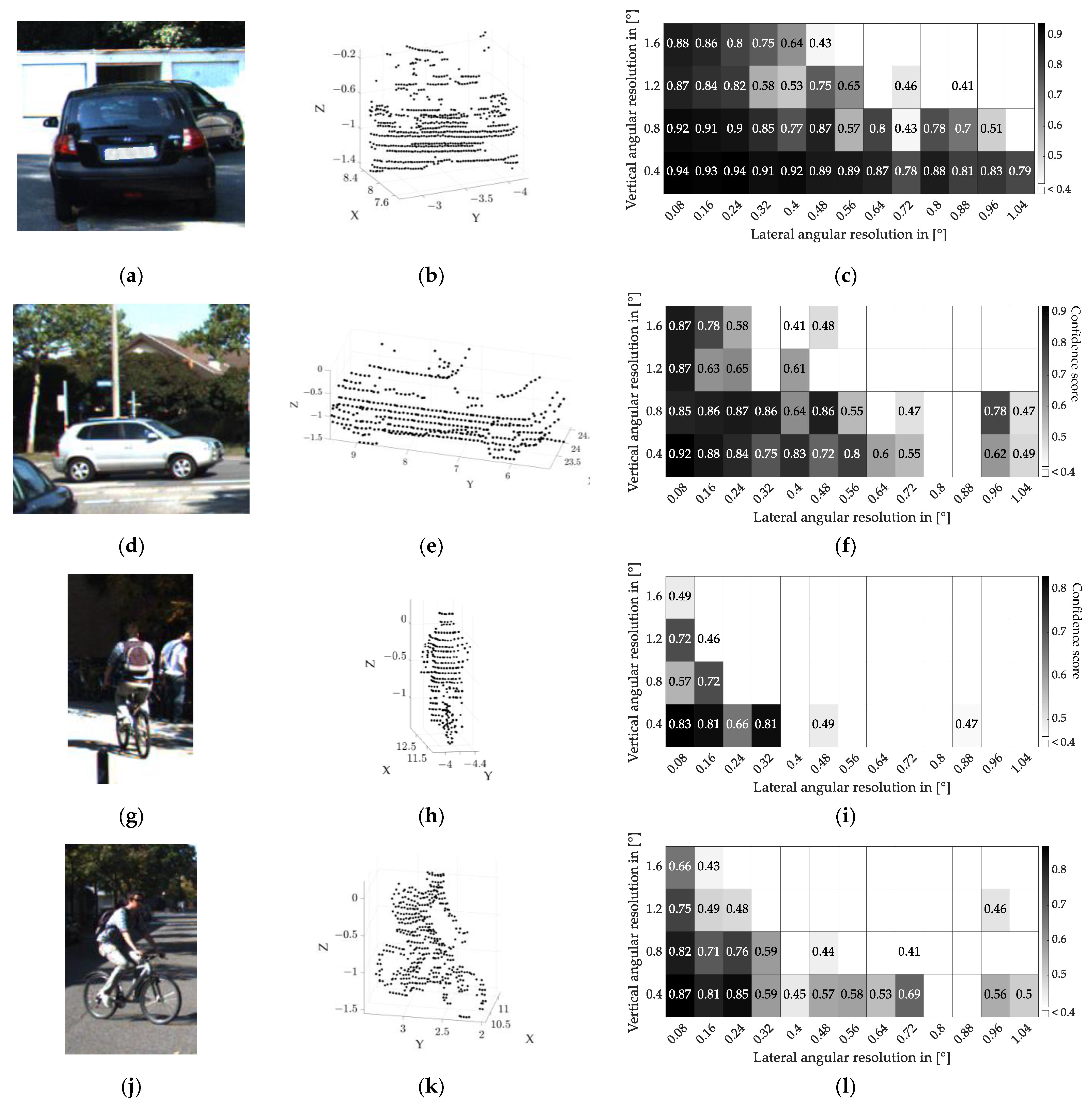
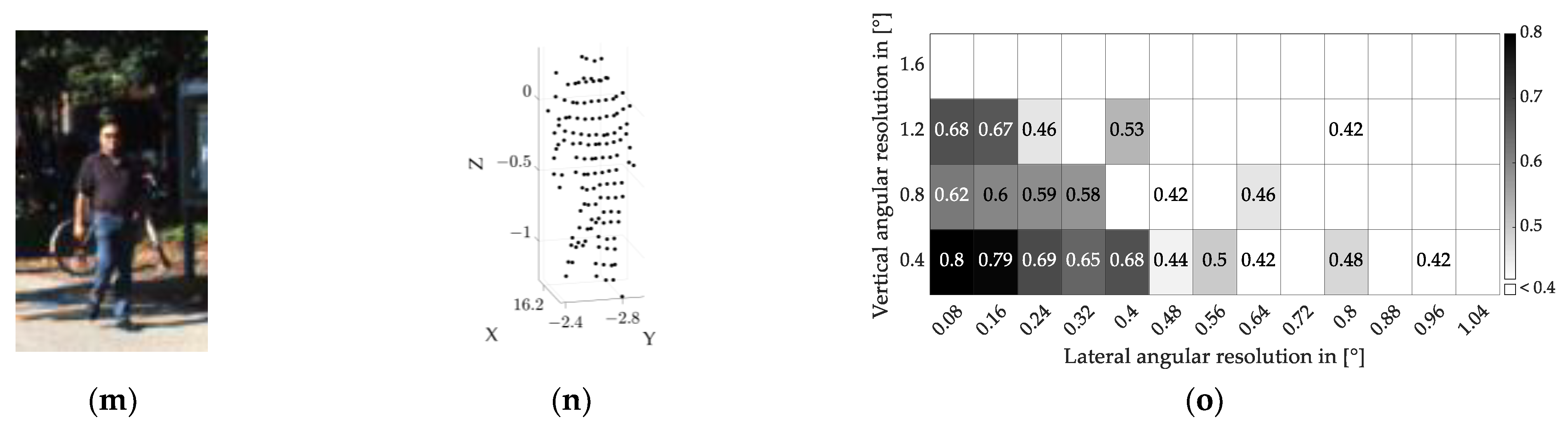
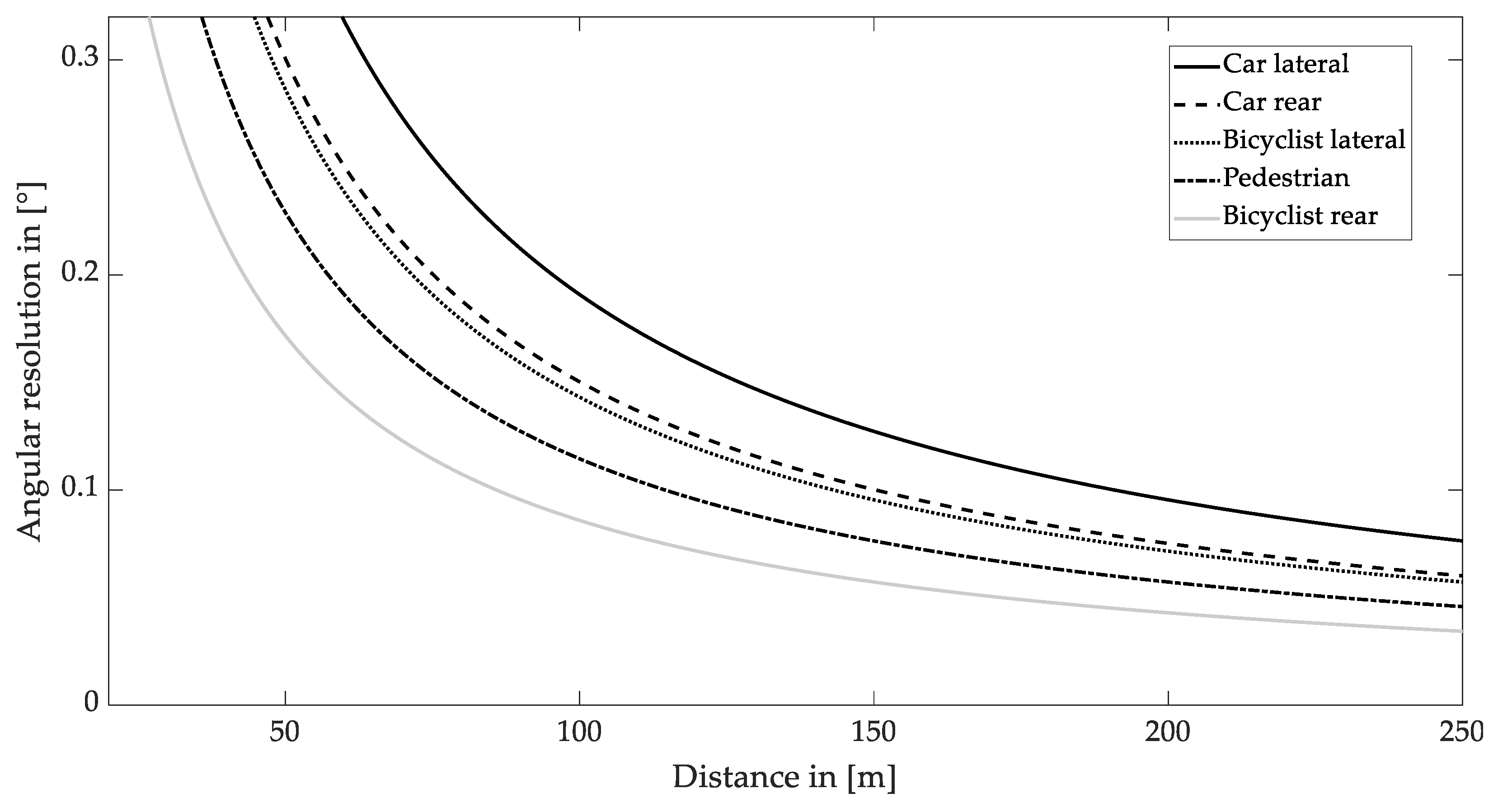
4.3. Angular Resolution Requirements
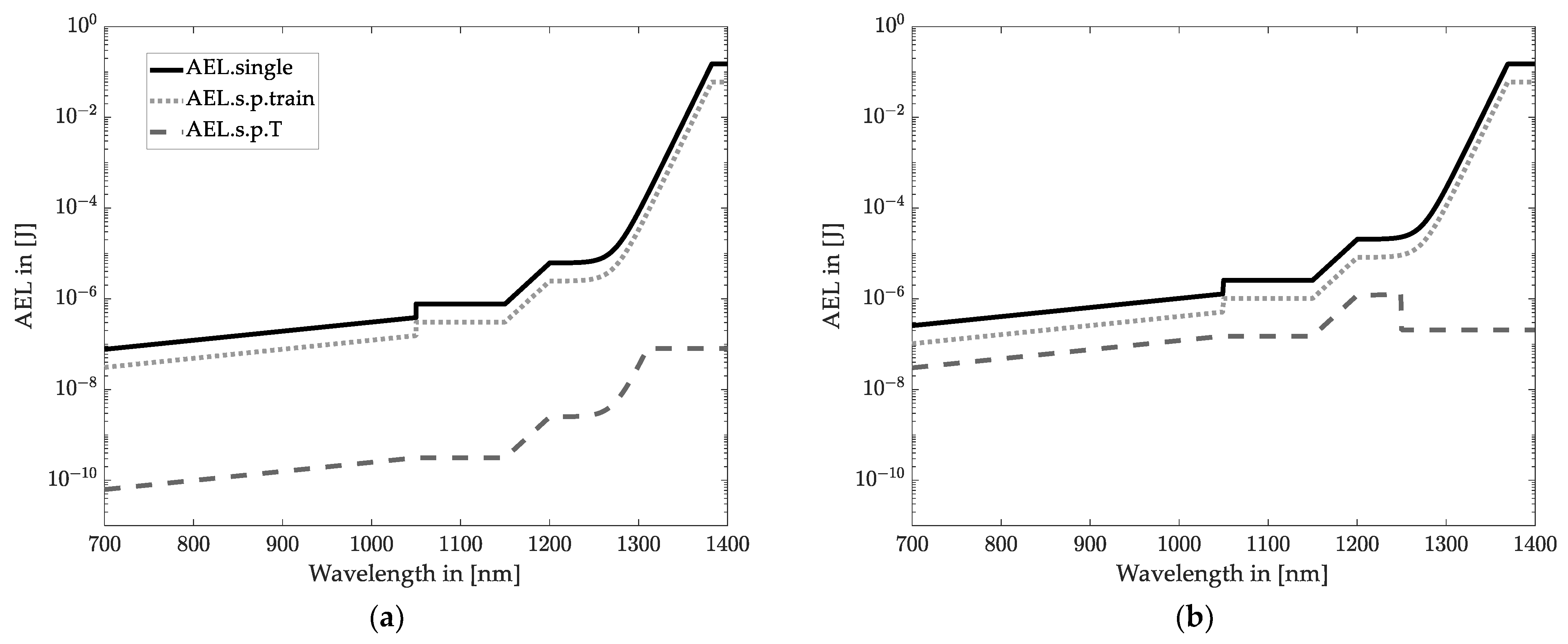
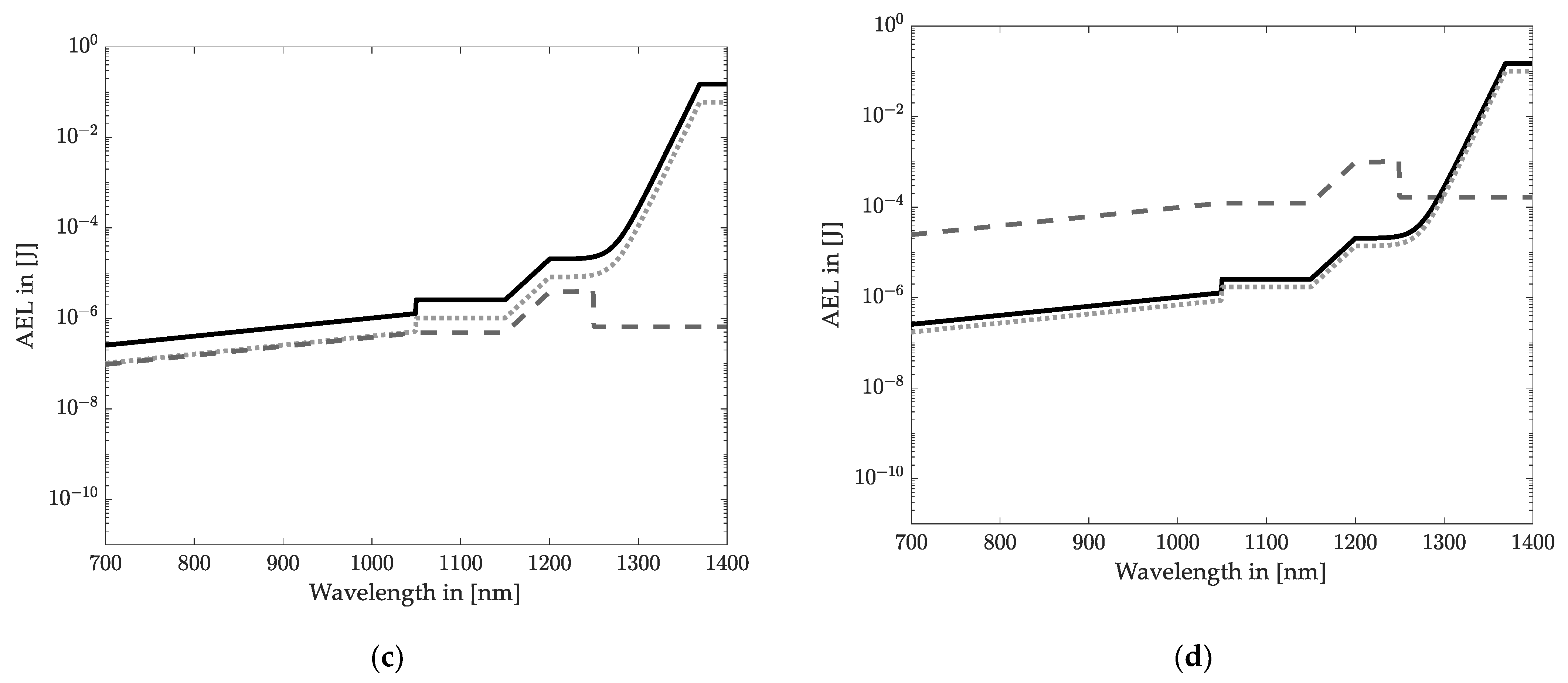
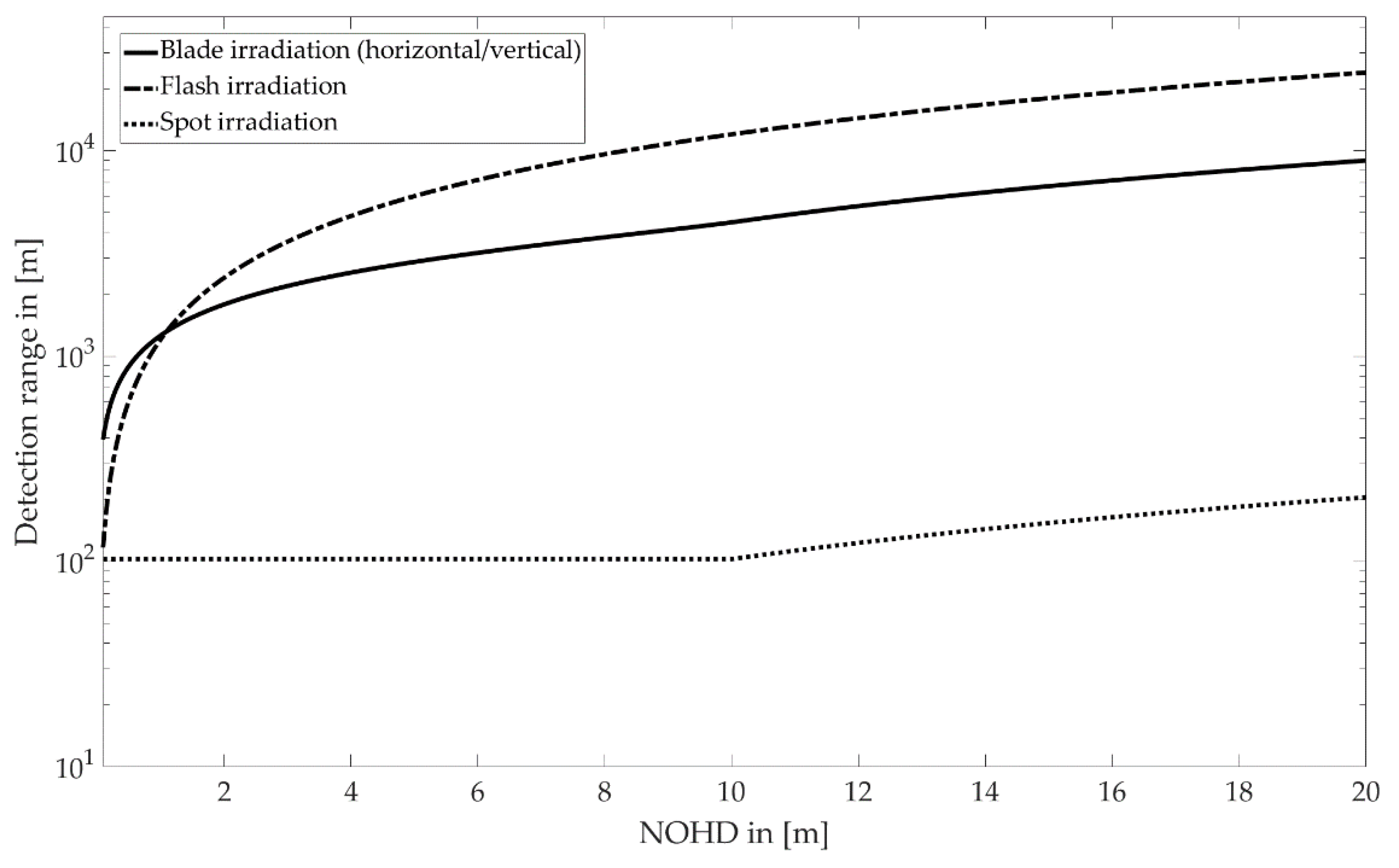
4.4. Laser Safety and Comparison of the Detection Range
- Wavelength;
- Pulse duration;
- Frame rate;
- Number of pulses per frame;
- Laser beam divergence.
- The maximum AEL for a single pulse (AEL.single);
- The average power for a pulse train (AEL.s.p.T) of an emission duration T;
- The AEL for a single pulse multiplied by a correction factor C5 (AEL.s.p.train).
- Pixel number: 815 × 255;
- Frame rate: 30 Hz;
- Beam divergence in spot scanning LiDAR systems: <1.5 mrad;
- Single pulse duration: 5 ns;
- Number of light sources for each pattern: 1.
- Laser wavelength: 905 nm.
- Laser divergence angle:
- ○
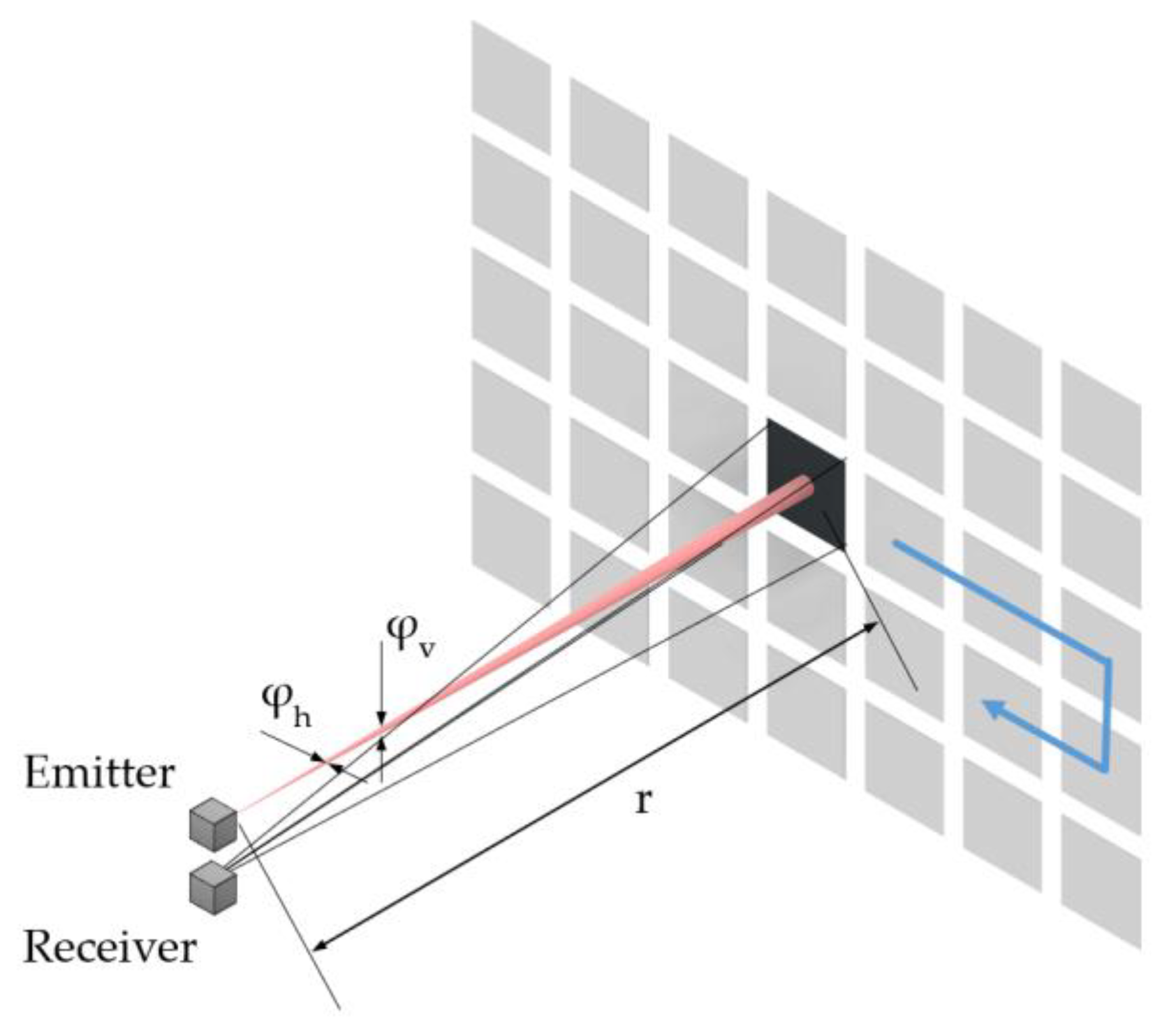
- spot scanning: 0.04° × 0.04° (equals the resolution requirement);
- ○
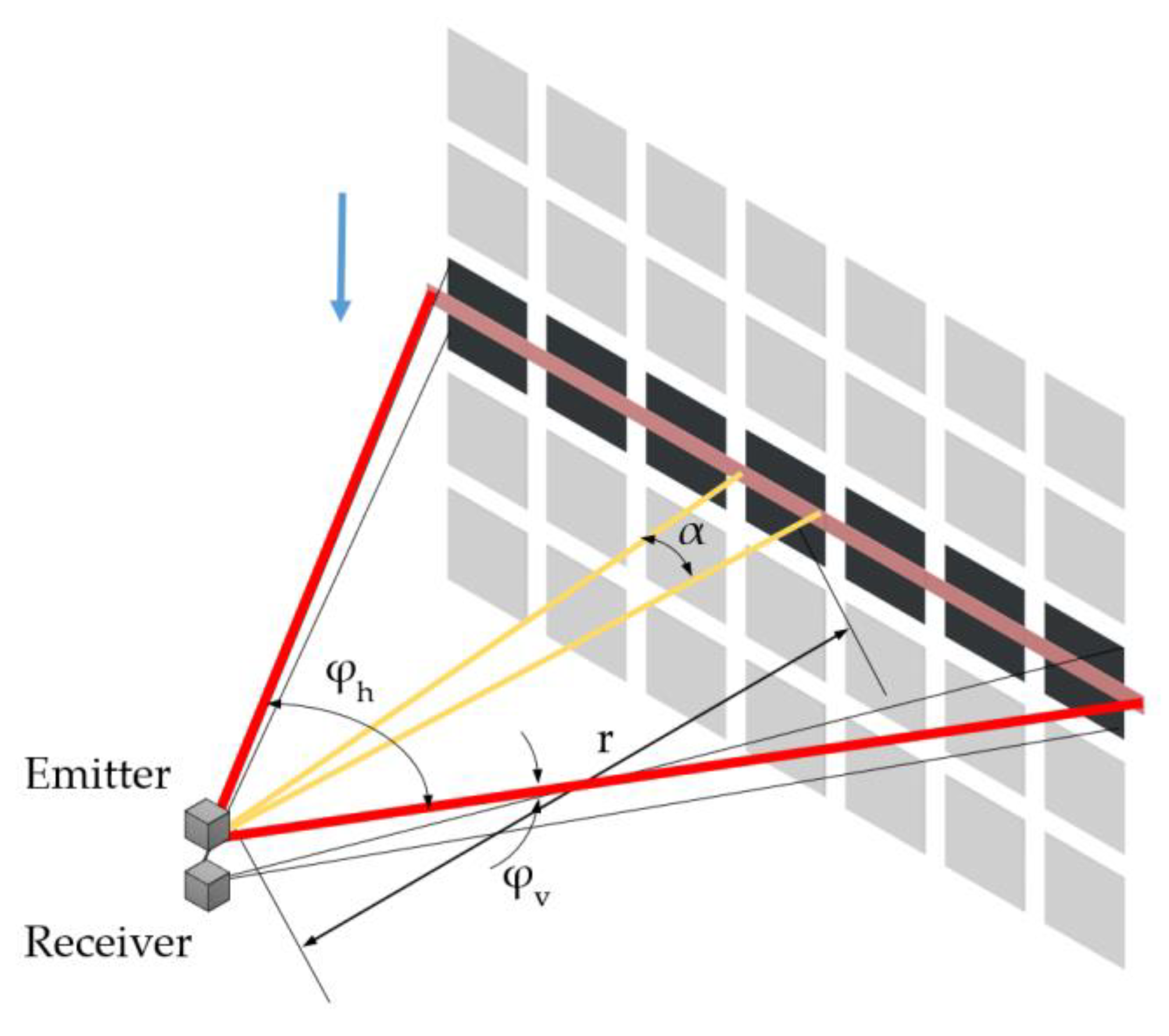
- blade irradiation, horizontal scanning: 0.04° × 10.2°;
- ○
- blade irradiation, vertical scanning: 32.6° × 0.04°;
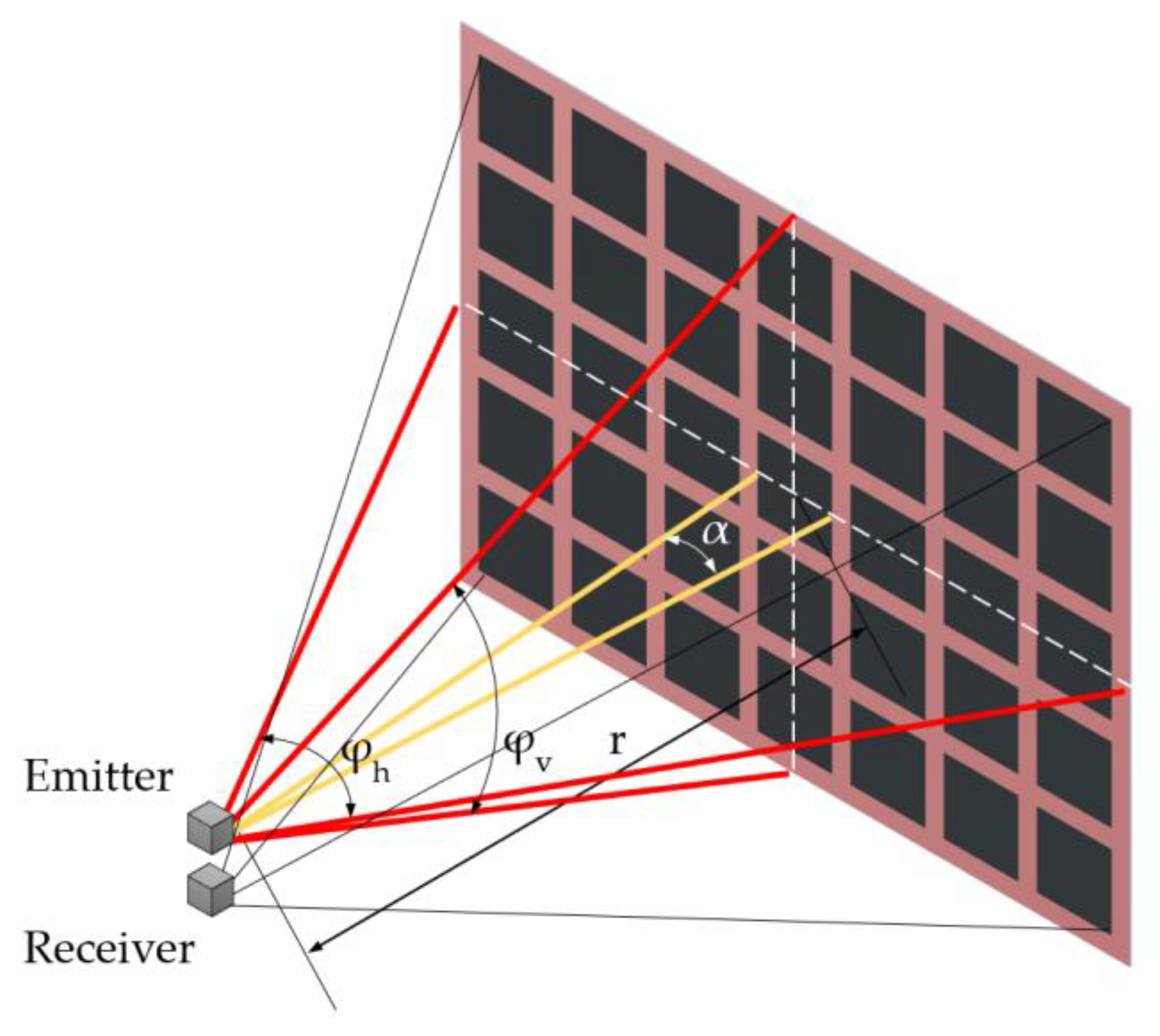
- ○
- flash irradiation: 32.6° × 10.2° (equals the FOV).
- Optical efficiency of the emitter: 90%.
- Optical efficiency of the detector: 90%.
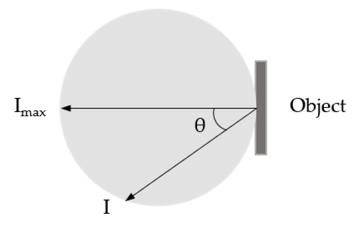
- Reflectivity of the object: 10% with Lambertian scattering characteristic (Section 3).
- Aperture of detector optical system: Ø 25.4 mm (1′′).
- Pupil diameter: Ø 7 mm.
- Atmospheric attenuation and scattering: neglected.
- Pixel gap: neglected.
- Intensity distribution of the emitter: homogeneous, K = 1.
5. Discussion
6. Conclusions
Author Contributions
Funding
Institutional Review Board Statement
Informed Consent Statement
Data Availability Statement
Acknowledgments
Conflicts of Interest
Appendix A
Appendix A.1. Lambertian Backscatter

Appendix A.2. Spot Irradiation

Appendix A.3. Blade Irradiation

Appendix A.4. Flash Irradiation

References
- Hecht, J. LiDAR for self-driving cars. Opt. Photonics News 2018, 29, 26–33. [Google Scholar] [CrossRef]
- Stann, B.L.; Dammann, J.F.; Giza, M.M.; Jian, P.S.; Lawler, W.B.; Nguyen, H.M.; Sadler, L.C. MEMS-scanned ladar sensor for small ground robots. In Laser Radar Technology and Applications XV; International Society for Optics and Photonics: Orlando, FL, USA, 2010; Volume 7684, p. 76841E. [Google Scholar] [CrossRef]
- Chung, S.; Abediasl, H.; Hashemi, H. A Monolithically Integrated Large-Scale Optical Phased Array in Silicon-on-Insulator CMOS. IEEE J. Solid-State Circuits 2018, 53, 275–296. [Google Scholar] [CrossRef]
- Halterman, R.; Bruch, M. Velodyne HDL-64E lidar for unmanned surface vehicle obstacle detection. In Unmanned Systems Technology XII; International Society for Optics and Photonics: Orlando, FL, USA, 2010; Volume 7692, p. 76920D. [Google Scholar] [CrossRef]
- Hao, Q.; Tao, Y.; Cao, J.; Cheng, Y. Development of pulsed-laser three-dimensional imaging flash lidar using APD arrays. Microw. Opt. Technol. Lett. 2021, 63, 2492–2509. [Google Scholar] [CrossRef]
- Warren, M.E. Automotive LIDAR technology. In Proceedings of the 2019 Symposium on VLSI Circuits, Kyoto, Japan, 9–14 June 2019; IEEE: New York, NY, USA, 2019; pp. C254–C255. [Google Scholar] [CrossRef]
- Wang, D.; Watkins, C.; Xie, H. MEMS mirrors for LiDAR: A review. Micromachines 2020, 11, 456. [Google Scholar] [CrossRef]
- Poulton, C.V.; Byrd, M.J.; Russo, P.; Timurdogan., E.; Khandaker., M.; Vermeulen., D.; Watts, M.R. Long-range LiDAR and free-space data communication with high-performance optical phased arrays. IEEE J. Sel. Top. Quantum Electron. 2019, 25, 1–8. [Google Scholar] [CrossRef]
- Zhao, F.; Jiang, H.; Liu, Z. Recent development of automotive LiDAR technology, industry and trends. In Proceedings of the Eleventh International Conference on Digital Image Processing, Guangzhou, China, 10–13 May 2019; Volume 11179, p. 111794A. [Google Scholar] [CrossRef]
- Yeong, D.J.; Velasco-Hernandez, G.; Barry, J.; Walsh, J. Sensor and sensor fusion technology in autonomous vehicles: A review. Sensors 2021, 21, 2140. [Google Scholar] [CrossRef]
- Xu, F.; Qiao, D.; Xia, C.; Song, X.; Zheng, W.; He, Y.; Fan, Q. A semi-coaxial MEMS LiDAR design with independently adjustable detection range and angular resolution. Sens. Actuators A Phys. 2021, 326, 112715. [Google Scholar] [CrossRef]
- Hsu, C.P.; Li, B.; Rivas, B.S.; Gohil, A.; Chan, P.H.; Moore, A.D.; Donzella, V. A review and perspective on optical phased array for automotive LiDAR. IEEE J. Sel. Top. Quantum Electron. 2020, 27, 8300416. [Google Scholar] [CrossRef]
- Takashima, Y.; Hellman, B. Review paper: Imaging lidar by digital micromirror device. Opt. Rev. 2020, 27, 400–408. [Google Scholar] [CrossRef]
- Raj, T.; Hashim, F.H.; Huddin, A.B.; Ibrahim, M.F.; Hussain, A. A Survey on LiDAR Scanning Mechanisms. Electronics 2020, 9, 741. [Google Scholar] [CrossRef]
- IEC 60825-1; Safety of Laser Products—Part 1: Equipment Classification and Requirements. IEC: Geneva, Switzerland, 2014.
- Royo, S.; Ballesta-Garcia, M. An Overview of Lidar Imaging Systems for Autonomous Vehicles. Appl. Sci. 2019, 9, 4093. [Google Scholar] [CrossRef] [Green Version]
- Dummer, M.; Johnson, K.; Rothwell, S.; Tatah, K.; Hibbs-Brenner, M. The role of VCSELs in 3D sensing and LiDAR. In Optical Interconnects XXI; International Society for Optics and Photonics: Orlando, FL, USA, 2021; Volume 11692, p. 116920C. [Google Scholar] [CrossRef]
- Eichler, H.J.; Eichler, J. Laser: Bauformen, Strahlführung, Anwendungen; Springer: Berlin/Heidelberg, Germany, 2015; p. 370. [Google Scholar] [CrossRef]
- McManamon, P.F.; Banks, P.S.; Beck, J.D.; Fried, D.G.; Huntington, A.S.; Watson, E.A. Comparison of flash LiDAR detector options. Opt. Eng. 2017, 56, 031223. [Google Scholar] [CrossRef] [Green Version]
- McManamon, P.F. Field Guide to LiDAR; SPIE Press: Bellingham, WA, USA, 2015; ISBN 9781628416541. [Google Scholar]
- Pulikkaseril, C.; Lam, S. Laser eyes for driverless cars: The road to automotive LIDAR. In Proceedings of the Optical Fiber Communication Conference, San Diego, CA, USA, 3–7 March 2019; Optical Society of America: San Diego, CA, USA, 2019; pp. 1–4. [Google Scholar] [CrossRef]
- Villa, F.; Severini, F.; Madonini, F.; Zappa, F. SPADs and SiPMs Arrays for Long-Range High-Speed Light Detection and Ranging (LiDAR). Sensors 2021, 21, 3839. [Google Scholar] [CrossRef] [PubMed]
- Kloppenburg, G.; Wolf, A.; Lachmayer, R. High-resolution vehicle headlamps: Technologies and scanning prototype. Adv. Opt. Technol. 2016, 5, 147–155. [Google Scholar] [CrossRef] [Green Version]
- Ley, P.P.; Lachmayer, R. Imaging and non-imaging illumination of DLP for high resolution headlamps. In Emerging Digital Micromirror Device Based Systems and Applications XI; International Society for Optics and Photonics: San Francisco, CA, USA, 2019; Volume 10932, p. 109320O. [Google Scholar] [CrossRef]
- Kutila, M.; Pyykönen, P.; Ritter, W.; Sawade, O.; Schäufele, B. Automotive LIDAR sensor development scenarios for harsh weather conditions. In Proceedings of the 2016 IEEE 19th International Conference on Intelligent Transportation Systems (ITSC), Rio de Janeiro, Brazil, 1–4 November 2016; pp. 265–270. [Google Scholar] [CrossRef]
- Wolf, A.; Kloppenburg, G.; Danov, R.; Lachmayer, R. DMD Based Automotive Lighting Unit. In Proceedings of the DGaO Proceedings, Hannover, Germany, 17–21 May 2016. [Google Scholar] [CrossRef]
- Knöchelmann, M.; Wolf, A.; Kloppenburg, G.; Lachmayer, R. Aktiver Scheinwerfer mit DMD-Technologie zur Erzeugung vollständiger Lichtverteilungen. VDI Ber. 2018, 2323, 61–78. [Google Scholar] [CrossRef]
- Li, Y.; Wolf, A.; Lachmayer, R. Laser LCoS High-Resolution Headlamp. In Spatially, Temporally and Spectrally Adapted Light for Applications; TEWISS: Garbsen, Germany, 2020; pp. 33–35. ISBN 978-3-95900-424-4. [Google Scholar]
- ISO 15623:2013; Intelligent Transport Systems—Forward Vehicle Collision Warning Systems—Performance Requirements and test Procedures. International Organization for Standardization: Geneva, Switzerland, 2013.
- Gotzig, H.; Geduld, G.O. LIDAR-sensorik. In Handbuch Fahrerassistenzsysteme; ATZ/MTZ-Fachbuch; Springer Vieweg: Wiesbaden, Germany, 2015; pp. 317–334. [Google Scholar] [CrossRef]
- Thakur, R. Scanning LIDAR in Advanced Driver Assistance Systems and Beyond: Building a road map for next-generation LIDAR technology. IEEE Consum. Electron. Mag. 2016, 5, 48–54. [Google Scholar] [CrossRef]
- ISO 15622:2018; Intelligent Transport Systems—Adaptive Cruise Control Systems—Performance Requirements and Test Procedures. International Organization for Standardization: Geneva, Switzerland, 2018.
- Johansson, G.; Rumar, K. Drivers’ brake reaction times. Hum. Factors 1971, 13, 23–27. [Google Scholar] [CrossRef]
- Speed Limits by Country. Available online: https://en.wikipedia.org/wiki/Speed_limits_by_country (accessed on 24 January 2022).
- Forschungsgesellschaft für Straßen- und Verkehrswesen (FGSV). Richtlinien für die Anlage von Landstraßen. RASt 06; FGSV Verlag: Köln, Germany, 2012. [Google Scholar]
- Forschungsgesellschaft für Straßen- und Verkehrswesen (FGSV). Richtlinien für die Anlage von Stadtstraßen. RASt 06; FGSV Verlag: Köln, Germany, 2008. [Google Scholar]
- Gut, C.; Cristea, I.; Neumann, C. High-resolution headlamp. Adv. Opt. Technol. 2016, 5, 109–116. [Google Scholar] [CrossRef]
- Geiger, A.; Lenz, P.; Stiller, C.; Urtasun, R. Vision meets robotics: The kitti dataset. Int. J. Robot. Res. 2013, 32, 1231–1237. [Google Scholar] [CrossRef]
- Shi, S.; Guo, C.; Jiang, L.; Wang, Z.; Shi, J.; Wang, X.; Li, H. Pv-rcnn: Point-voxel feature set abstraction for 3d object detection. In Proceedings of the IEEE/CVF Conference on Computer Vision and Pattern Recognition, Seattle, WA, USA, 13–19 June 2020; pp. 10529–10538. [Google Scholar]
- Shi, S.; Wang, X.; Li, H. Pointrcnn: 3D object proposal generation and detection from point cloud. In Proceedings of the IEEE/CVF Conference on Computer Vision and Pattern Recognition, Long Beach, CA, USA, 15–20 June 2019; pp. 770–779. [Google Scholar]
- Yan, Y.; Mao, Y.; Li, B. Second: Sparsely embedded convolutional detection. Sensors 2018, 18, 3337. [Google Scholar] [CrossRef] [Green Version]
- Lang, A.H.; Vora, S.; Caesar, H.; Zhou, L.; Yang, J.; Beijbom, O. Pointpillars: Fast encoders for object detection from point clouds. In Proceedings of the IEEE/CVF Conference on Computer Vision and Pattern Recognition, Long Beach, CA, USA, 15–20 June 2019; pp. 12697–12705. [Google Scholar]
- Simonelli, A.; Bulo, S.R.; Porzi, L.; López-Antequera, M.; Kontschieder, P. Disentangling monocular 3d object detection. In Proceedings of the IEEE/CVF International Conference on Computer Vision, Seoul, Korea, 27 October–2 November 2019; pp. 1991–1999. [Google Scholar]
- Maksymova, I.; Steger, C.; Druml, N. Review of LiDAR Sensor Data Acquisition and Compression for Automotive Applications. Proceedings 2018, 2, 852. [Google Scholar] [CrossRef] [Green Version]
- Everingham, M.; Van Gool, L.; Williams, C.K.; Winn, J.; Zisserman, A. The pascal visual object classes (voc) challenge. Int. J. Comput. Vis. 2010, 88, 303–338. [Google Scholar] [CrossRef] [Green Version]
- Redmon, J.; Divvala, S.; Girshick, R.; Farhadi, A. You only look once: Unified, real-time object detection. In Proceedings of the IEEE Conference on Computer Vision and Pattern Recognition, Las Vegas, NV, USA, 27–30 June 2016; pp. 779–788. [Google Scholar]
- Kutila, M.; Pyykönen, P.; Holzhüter, H.; Colomb, M.; Duthon, P. Automotive LiDAR performance verification in fog and rain. In Proceedings of the 2018 21st International Conference on Intelligent Transportation Systems (ITSC), Maui, HI, USA, 4–7 November 2018; pp. 1695–1701. [Google Scholar] [CrossRef]
- Knigge, A.; Klehr, A.; Wenzel, H.; Zeghuzi, A.; Fricke, J.; Maaßdorf, A.; Tränkle, G. Wavelength-stabilized high-pulse-power laser diodes for automotive LiDAR. Phys. Status Solidi 2018, 215, 1700439. [Google Scholar] [CrossRef]
- Winner, H.; Schopper, M. Adaptive Cruise Control. In Handbuch Fahrerassistenzsysteme; ATZ/MTZ-Fachbuch; Springer Vieweg: Wiesbaden, Germany, 2015; pp. 851–890. [Google Scholar] [CrossRef]
- Qasem, S.N.; Ahmadian, A.; Mohammadzadeh, A.; Rathinasamy, S.; Pahlevanzadeh, B. A type-3 logic fuzzy system: Optimized by a correntropy based Kalman filter with adaptive fuzzy kernel size. Inf. Sci. 2021, 572, 424–443. [Google Scholar] [CrossRef]


| Symbol | Quantity | Units |
|---|---|---|
| Received power | W | |
| Emitted power | W | |
| Atmospheric transmission | - | |
| Optical efficiency of the emitter | - | |
| Beam spread area of the emitter at the target | m2 | |
| Target cross-section | m2 | |
| Reflectance of the target | - | |
| Distance between LiDAR and the target | m | |
| Optical aperture of the receiver | m2 | |
| Optical efficiency of the receiver | - |
| Case | Beam Spread Area | Cross-Section | Range Equation |
|---|---|---|---|
| Spot irradiation | |||
| Blade irradiation | |||
| Flash irradiation |
| No. | Scenario | Warning Distance |
|---|---|---|
| 1 | Preceding vehicle travels at ordinary speed | |
| 2 | Preceding vehicle is stationary | |
| 3 | Preceding vehicle decelerates with a relative speed |
| Curve Class | Curve Radius | Full Horizontal FOV | Full Vertical FOV |
|---|---|---|---|
| Class Ⅰ | ≥500 m | 12.4° | 5.2° |
| Class Ⅱ | ≥250 m | 18.0° | 6.8° |
| Class Ⅲ | ≥125 m | 32.6° | 10.2° |
| Algorithms | Average Precision | Processing Time per Image (GPU/CPU) | ||
|---|---|---|---|---|
| Cars | Pedestrians | Bicyclists | ||
| PV-RCNN [39] | 94.10% | 66.38% | 75.77% | 0.1837 s/0.1726 s |
| PointRCNN [40] | 92.90% | 75.03% | 76.76% | 0.0861 s/0.0851 s |
| SECOND [41] | 94.51% | 71.94% | 76.50% | 0.0487 s/0.0488 s |
| PointPillars [42] | 93.91% | 65.46% | 72.34% | 0.0270 s/0.0286 s |
| Object | Perspective | Aspect Ratio (B:H) | Min. Required Points | Min. Pixel Number |
|---|---|---|---|---|
| Car | Rear | 2:1 | 31 | 8 × 4 |
| Lateral | 4:1 | 25 | 12 × 3 | |
| Bicyclist | Rear | 1:3 | 46 | 4 × 12 |
| Lateral | 7:6 | 48 | 8 × 6 | |
| Pedestrian | - | 3:8 | 14 | 3 × 8 |
Publisher’s Note: MDPI stays neutral with regard to jurisdictional claims in published maps and institutional affiliations. |
© 2022 by the authors. Licensee MDPI, Basel, Switzerland. This article is an open access article distributed under the terms and conditions of the Creative Commons Attribution (CC BY) license (https://creativecommons.org/licenses/by/4.0/).
Share and Cite
Dai, Z.; Wolf, A.; Ley, P.-P.; Glück, T.; Sundermeier, M.C.; Lachmayer, R. Requirements for Automotive LiDAR Systems. Sensors 2022, 22, 7532. https://doi.org/10.3390/s22197532
Dai Z, Wolf A, Ley P-P, Glück T, Sundermeier MC, Lachmayer R. Requirements for Automotive LiDAR Systems. Sensors. 2022; 22(19):7532. https://doi.org/10.3390/s22197532
Chicago/Turabian StyleDai, Zhuoqun, Alexander Wolf, Peer-Phillip Ley, Tobias Glück, Max Caspar Sundermeier, and Roland Lachmayer. 2022. "Requirements for Automotive LiDAR Systems" Sensors 22, no. 19: 7532. https://doi.org/10.3390/s22197532
APA StyleDai, Z., Wolf, A., Ley, P.-P., Glück, T., Sundermeier, M. C., & Lachmayer, R. (2022). Requirements for Automotive LiDAR Systems. Sensors, 22(19), 7532. https://doi.org/10.3390/s22197532